A New Method for Dynamical System Identification by Optimizing the Control Parameters of Legendre Multiwavelet Neural Network

Abstract

Wavelet neural networks have been widely applied to dynamical system identification fields. The most difficult issue lies in selecting the optimal control parameters (the wavelet base type and corresponding resolution level) of the network structure. This paper utilizes the advantages of Legendre multiwavelet (LW) bases to construct a Legendre multiwavelet neural network (LWNN), whose simple structure consists of an input layer, hidden layer, and output layer. It is noted that the activation functions in the hidden layer are adopted as LW bases. This selection if based on the its rich properties of LW bases, such as piecewise polynomials, orthogonality, various regularities, and more. These properties contribute to making LWNNs more effective in approximating the complex characteristics exhibited by uncertainties, step, nonlinear, and ramp in the dynamical systems compared to traditional wavelet neural networks. Then, the number of selection LW bases and the corresponding resolution level are effectively optimized by the simple Genetic Algorithm, and the improved gradient descent algorithm is implemented to learn the weight coefficients of LWNN. Finally, four nonlinear dynamical system identification problems are applied to validate the efficiency and feasibility of the proposed LWNN-GA method. The experiment results indicate that the LWNN-GA method achieves better identification accuracy with a simpler network structure than other existing methods.

1. Introduction

Nonlinear dynamical system identification is very important in various engineering applications [1,2]. Several system identification approaches, encompassing both mathematical model-based and data-driven methods, have been developed to solve this difficult problem posed by the complex characteristics of dynamical systems, which often exhibit high nonlinearity, uncertainties, delays, step, disturbances, and more [3,4,5,6]. Among the various methods for system identification, as it is difficult to establish an accurate mathematical model for the dynamical systems, the data-driven methods based on intelligent methods concerned in this study have recently been widely accepted and applied in the nonlinear dynamical system identification fields [2,7,8]. Various intelligent methods such as neural networks (NN) based on biological knowledge, fuzzy systems based on the operator’s knowledge with respect to the dynamical systems, fuzzy neural networks (FNN) [9,10,11,12,13], wavelet neural networks (WNN) [14,15,16], fuzzy wavelet neural networks (FWNN), and more [17,18,19,20] have been implemented to identify the nonlinear dynamical systems, and succesful identification results have been attained.

It is known that different variants of NN, multi-layer perceptron NN (MLPNN), radial basis function network (RBFN), recurrent neural network (RNN) [19], long short-term memory (LSTM) network, and more, have been widely used for nonlinear dynamical system identification [21,22]. The main issue of the MLPNN model is that the weights adjustment does not exploit any of the local data structure, and the function approximation is very sensitive to the available training data [21]. The presence of a feedback loop in RNN enhances their ability to approximate nonlinear dynamical systems. RNNs are deemed some of the most attractive models for processing information generated by various of dynamical systems, successfully overcoming the disadvantages of the MLPNN model [22]. For example, Kumar proposed a memory recurrent Elman neural network-based method for the time-delayed nonlinear dynamical system identification [19]. It is noted that the other requirement from the identification model is that it should be robust, that is, it should be able to compensate for the effects of uncertainties such as parameter variations and disturbance signals. An adaptive sliding-mode control system using a double-loop RNN structure was proposed for a class of nonlinear dynamic systems in Ref. [23], which realized the merits of high precision, fast speed, and strong robustness. Chu and Fei [8] proposed an adaptive dynamic global sliding-mode controller based on a proportional integral derivative sliding surface using a radial basis function neural network (NN) for a three-phase active power filter to obtain global robustness. Ghahderijani et al. [24] presented a sliding-mode control scheme to provide high robustness to external disturbances and transient response with large and abrupt load changes.

Although the methods based on NN have the ability to approximate any deterministic nonlinear process with little knowledge and no assumptions [3,14,25], the processing of the random weight initialization is generally accompanied with extended training cost and the training algorithm will converge to the local minima. In particular, there is no theoretical relationship between the specific learning parameters of the network and the optimal network architecture [26]. To effectively solve these issues, WNN, i.e., an alternative NN, is proposed to alleviate the aforementioned weaknesses [27,28]. Usually, three types of wavelet bases, the Gaussian derivative, the second derivative of the Gaussian, and the Morlet wavelet, are suggested to construct WNN [29]. However, in order to obtain less iteration steps in the training procedure, and arrive at the global convergence minimum of the loss function, various approaches have been proposed to initialize the dilation and translation parameters of the wavelet bases as the activation functions of the network [30,31,32,33]. For example, Luo et al. developed an identification of autonomous nonlinear dynamical system based on discrete-time multiscale wavelet neural network [16]. Emami developed an identification of nonlinear time-varying systems using wavelet neural networks [34]. However, wavelet neural networks involve adjusting multiple parameters, including the selection of wavelet functions, determination of wavelet scales, and the number of layers and nodes in the neural network. Adjusting these parameters requires experimentation and optimization, often involving iterative attempts with different parameter combinations and evaluating the model’s performance using appropriate evaluation metrics.

Additionally, FWNN contains the advantages of both the fuzzy systems and WNN, which can decrease the number of rules significantly. It has been successfully applied in the dynamical system identification [35,36]. For example, Wang et al. combined the fuzzy-neural structure with long short-term memory (LSTM) mechanism to identify the nonlinear dynamical system [37]. However, FWNN needs a large number of neurons to obtain a reasonably good performance in the nonlinear dynamical system identification, which increases the dimension and configuration parameters of the network [38,39,40].

Consequently, it is very necessary to design a new effective neural network and optimize the control parameters of the network structure, so as to effectively identify the nonlinear dynamical system. Fortunately, attractive properties such as piecewise polynomials, compact support, orthogonality, and various regularities of LW bases, constructed by Alpert et al. [41], provide an alternative structure for WNN. These properties are very beneficial for constructing a simpler and lower computational complexity network.

In this paper, our main objective is to design a LWNN based on the advantages of LW base functions and optimize the control parameters, i.e., the number of LW bases and corresponding resolution levels of this network, using a simple Genetic Algorithm, which enhances the effectiveness and adaptability of the network applied to the nonlinear dynamical system identification. More precisely, the basic structure of LWNN is composed of the input layer, hidden layer, and output layer, which are described in Figure 1 in detail. Due to the compact support and orthogonality properties of LW bases, the input data are parted into some subsections according to the optimal resolution level, which leads to locally connecting and sharing weights in each subsection, decreasing the calculation cost in the procedure of the network training. In the hidden layer, the essence of each main neuron is a linear combination of LW bases. Therefore, the number of LW bases and the resolution level measure the complexity of LWNN structure. The two control parameters of the network are optimized by the simple Genetic Algorithm to effectively and adaptively learn the salient features of the nonlinear dynamical system. In particular, the number of LW base functions and resolution level are usually small positive integers, and they are easy to optimize using the simple Genetic Algorithm rather than the various complex algorithms for initialization of the dilation and translation parameters used in the traditional WNN [37]. The performance of the LWNN-GA method is supported by rigorous wavelet analysis theory, and any function in $L_2\left([0,1]\right)$ can be approximated with any accuracy through sufficient training of LWNN [41].

To summarize, in comparison to other neural networks, the contribution of our proposed method terms of the NN model are mainly due to the theoretical guidance, local learning structure, and adaptive adjustment mechanism, which makes the network topology more compact and simpler with a single hidden layer, attaining a high learning efficiency.

In order to demonstrate the effectiveness and feasibility of the proposed method in this article, the improved gradient descent algorithm is implemented to learn the network weight coefficients of the optimized structure model by the simple Genetic Algorithm, which can effectively approximate a benchmark piecewise function and identify three nonlinear dynamical systems. The main contributions of this paper are listed as follows:

(1)

This paper proposes a simplified LWNN to identify the nonlinear dynamical system. In essence, the main neuron in the hidden layer is a linear combination of orthogonal explicit LW polynomial bases instead of the traditional non-polynomial activation functions, which can effectively decrease the number of learning weight coefficients and avoid the issue of the numerical instability in the nonlinear dynamical system identification process;

(2)

The two control parameters of this network are optimized by the simple Genetic Algorithm. To be specific, the resolution level and order of LW bases are optimized to attain the optimal network structure, and the improved gradient descent algorithm is utilized to learn the network weight coefficients, which are prior and simpler to the algorithms used by the traditional WNN;

(3)

The essential attribute of the adaptive piece-wise polynomial approximation enables the proposed method to locally connect and share weights involving only a small subset of LW coefficients. This local process structure effectively decreases the training cost with the improved gradient descent algorithm;

(4)

Various LW bases with rich vanishing moments and regularities provide a strong approximation tool to thoroughly learn the complex characteristics shown by the uncertainties, step, ramp, and disturbances in a nonlinear dynamical system. Especially, the approximation error converges exponentially according to the optimal resolution level and order of LW bases.

As demonstrated by the numerical experiment results in Section 4, the proposed method attains better identification accuracy than other complex neural networks, showing great potential for complex nonlinear system identification.

The remaining of this paper is organized as follows: Section 2 introduces the rich properties of LW bases, and the basic structure of LWNN is elaborately designed. Section 3 uses the simple Genetic Algorithm to optimize the order of the adopted LW bases and the resolution level. Then, the weight coefficients of the optimal LWNN structure are learned by the improved gradient descent algorithm. Finally, the detailed flowchart of the proposed method for identifying the nonlinear dynamic system is described. In Section 4, the performance evaluation measure of the experiment results is described. Then, the nonlinear dynamical system identification commonly used in the literature is implemented to verify the effectiveness of the proposed method. Finally, Section 5 gives some conclusions of this research and prospects for future work.

2. Legendre Multiwavelet Neural Network

In this section, the concept and properties of LW bases are first introduced. In the second step, the type of the nonlinear dynamical system identification is described. Finally, the basic structure of LWNN is specifically designed in this context.

2.1. Legendre Multiwavelet Bases

In this context, let $L_k\left(x\right)$ denote the Legendre polynomials of order k, which are defined as

$$\begin{array}{cc}\hfill L_0\left(x\right)=& 1,L_1\left(x\right)=x,\hfill \\ \hfill L_{k+2}\left(x\right)=& \frac{2k+3}{k+2}x{L}_{x+1}\left(x\right)-\frac{k+1}{k+2}{L}_k\left(x\right).\hfill \end{array}$$

(1)

By using simple transformation [42], LW bases defined on the resolution level 0 can be obtained as follows

$${\varphi }_k\left(x\right)=\left\{\begin{array}{cc}\sqrt{2k+1}{L}_k(2x-1),\hfill & x\in [0,1),\hfill \\ 0,\hfill & x\notin [0,1),\hfill \end{array}\right.$$

(2)

where the whole set ${\left\{{\varphi }_k\right\}}_{k=0}^{p-1}$ forms an orthogonal base for subspace $V_{p,0}$ and $p=1,2,\cdots$.

Then, for the resolution level $n=0,1,2,...$ and the corresponding translation $l=0,1,2,...,2^n-1$, define interval $I_{nl}=[2^{-n}l,2^{-n}(l+1)).$ Usually, the subspace $V_{p,n}$ is spanned by $2^{n}p$ base functions, which are obtained from ${\varphi }_0,...,{\varphi }_{k-1}$ by dilation and translation, i.e.,

$$V_{p,n}:=V_{p,n}=span\left\{{\varphi }_{k,nl}\left(x\right)=2^{n/2}{\varphi }_{k,n}(2^{n}x-l),0\le k\le p-1,0\le l\le 2^n-1\right\},$$

(3)

which forms an orthogonal base for $L_2\left([0,1\right]).$

2.2. Type of Nonlinear System Identification

In this subsection, the mathematical model of the nonlinear dynamical system identified in this paper is elaborately described as follows.

$$y(x+1)=f[y\left(x\right),y(x-1),\cdots ,y(x-j+1)]+\sum _{i=0}^m{c}_{i}u(x-i),$$

(4)

where f is usually unknown and operates on the input x and generates an output y. Then, $y(x+1)$ denotes one step ahead value of the nonlinear dynamical system, j denotes the order of the plant and $m\le j$, and $u\left(x\right)$ represents the present input to the nonlinear dynamical system.

It is noted that the issue of the nonlinear dynamical system identification is then to find an approximate form of f. In this paper, the proposed LWNN is used as an identifier of this nonlinear dynamical system, the strict mathematical theory foundation is described as: Any a function $f\in L_2\left([0,1]\right)$ is approximated by LW bases as the form [40]

$$∥f-\sum _{l=0}^{2^n-1}\sum _{k=0}^{p-1}{s}_{k,nl}{\varphi }_{k,nl}\left(x\right)∥\sim O\left(2^{-np}\right),$$

(5)

which demonstrates that the approximation error exponentially convergences with the resolution level n and order p of LW bases, which is very beneficial to construct the simpler and lower computational complexity network. Based on the calculation technique, the approximation coefficients $s_{k,nl}$ can be computed by the integral approach as

$$s_{k,nl}={\int }_{I,nl}f\left(x\right){\varphi }_{k,nl}\left(x\right)dx.$$

(6)

However, based on the data-driven intelligence method in this paper, the discrete data pairs of x and $f\left(x\right)$ obtained from the nonlinear dynamical system are utilized to train LWNN to adaptively attain the above approximation coefficients.

2.3. Structure of the Legendre Multiwavelet Neural Network

In this subsection, the basic structure of LWNN is designed by combing NN with the rigorous approximation ability of LW bases according to (5). In contrast to the traditional NN, the activation function in the hidden layer is replaced by LW bases. Then, according to the approximation form in (5), the constructed LWNN is a three-layer feed-forward neural network, which consists of the input layer, hidden layer, and output layer illustrated in Figure 1 in detail. The operations involved in each layer of LWNN are elaborately described as follows.

Input layer: The resolution level n and the order p of the LW bases are first initialized. Then, the input data vector is parted into $2^n$ subintervals according to the resolution level n, which is denoted by $\mathbf{x}={[x_{I_{n0}},x_{I_{n1}},...,x_{I_{nl}},...,x_{I_{n(2^n-1)}}]}^T$. Second, the parted vector is fed into the $2^n$ neurons in the input layer. Finally, it is directly transmitted to the hidden layer.

Hidden layer: Each main neuron ${\varphi }_{p,nl}$ in this layer is essential to a linear combination of LW bases. Figure 2 shows the structure of the $lth$ main neuron, which contains p orthogonal LW bases.

As demonstrated in Figure 1 and  Figure 2, the input layer is locally connected with the hidden layer, and each main neuron shares the network weights.

Then, the output $y_{I_{nl}}$ of the $lth$ main neuron in the hidden layer fed to the output layer is described as

$$y_{I_{nl}}=\sum _{k=0}^{p-1}{s}_{k,nl}{\varphi }_{k,nl}\left(x_{I_{nl}}\right).$$

(7)

Output layer: The output of LWNN is calculated using the following form

$$y=\sum _{l=0}^{2^n-1}{y}_{I_{nl}}.$$

(8)

In the output layer, the identification result of the nonlinear dynamical system is estimated by (8), which is conducive to the rapid convergence and provides better identification accuracy compared with the traditional NN, WNN, and FWNN methods.

3. Optimal Algorithm of the Proposed Method

In this section, the two control parameters of the constructed LWNN are first optimized by the simple Genetic Algorithm. In the second step, the improved gradient descent algorithm is implemented to learn the weight coefficients of LWNN. Finally, the flowchart of the proposed method applied to the nonlinear dynamical system identification is elaborately described in Figure 3.

3.1. Optimal Control Parameters of LWNN

The essence of the structure complexity with respect to LWNN is absolutely dependent on the resolution level and the order of LW bases, which are usually small positive integers validated by many engineering applications based on wavelet methods [42]. In this subsection, the simple Genetic Algorithm is reliably implemented to optimize the two control parameters of LWNN, aiming to attain the optimal network structure without relying on a large number of numerical experiments.

In this context, each chromosome is composed of two types of genes, representing the resolution level and the order of LW bases, respectively, which denote a certain network structure of LWNN. More precisely, the devised chromosome in this paper includes three genes and four genes for the resolution level and the order of LW bases, respectively, which are elaborately described in Figure 3. Furthermore, the fitness function is adopted as the identification accuracy of the nonlinear dynamical system. It is noted that the identification accuracy is attained by using the follow improved gradient descent algorithm to learn the weight coefficients of LWNN.

3.2. Learning Weight Coefficients of LWNN

Generally, a good training algorithm can decrease the training cost while achieving a better identification accuracy. In the present study, the improved gradient descent algorithm is used to learn the weight coefficients of LWNN, which is easy to compare with other methods for nonlinear dynamical system identification.

The traditional WNN learning process includes the complex calculations of the dilation and translation parameters of the wavelet activation functions and the weights optimization of the neural network [43]. However, in this context, the structure of LWNN is optimized by the above simple Genetic Algorithm to enhance the ability of adaptively learning the optimal network structure. The improved gradient descent algorithm is implemented to learn the weight coefficients between the hidden layer and the output layer of LWNN. To be specific, the purpose of the learning weight coefficients is to minimize the loss function, which is described as follows.

$$\begin{array}{cc}\hfill E& =\frac{1}{2}\sum _{l=0}^{2^n-1}{\left(f\left(x_{I_{nl}}\right)-y_{I_{nl}}\right)}^2,\hfill \\ \\ & =\frac{1}{2}\sum _{l=0}^{2^n-1}\sum _{k=0}^{p-1}{\left(f\left(x_{I_{nl}}\right)-s_{k,nl}{\varphi }_{k,nl}\left(x_{I_{nl}}\right)\right)}^2,\hfill \end{array}$$

(9)

where $f\left(x_{I_{nl}}\right)$ and $y_{I_{nl}}$ denote the actual values and output values of LWNN, respectively. The error E describes the difference between the actual values and the network output values.

Then, the partial derivative of the loss function with respect to the weight coefficients of LWNN is computed as

$$\frac{\partial E}{\partial s_{k,nl}}=-(f\left(x_{I_{nl}}\right)-s_{k,nl}{\varphi }_{k,nl}\left(x_{I_{nl}}\right)){\varphi }_{k,nl}\left(x_{I_{nl}}\right).$$

(10)

In fact, this network is trained until the optimal weight vector of theLW bases is found by minimizing the above loss function through iterative technique. To be specific, the above derivative of the loss function is calculated at each iteration step t. Then, the update of the weight coefficients is performed by the improved gradient descent algorithm, as follows.

$$s_{k,nl}^{t+1}=s_{k,nl}^t-\frac{\alpha }{m_l}\frac{\partial E^t}{\partial s_{k,nl}^t},t=1,2,...,N.$$

(11)

where $\alpha$ is the learning rate, which is constant, and $m_l$ is the number of the sample points in the subinterval $x_{I_{nl}}$, which enhances the learning speed due to the variation learning step with the sample points.

The network weight coefficients adjustment should end when the loss function reaches a fixed lower bound. If the number of iterations reaches a fixed maximum, then the learning process is complete. Accordingly, the optimal values of the resolution level n and the order p of LW bases for the structure of LWNN can be obtained by combing the simple Genetic Algorithm with this weight coefficients learning process.

3.3. The Flowchart of the Proposed Method

In essence, LWNN involves two important issues to be solved for the nonlinear dynamical system identification in this paper. Firstly, to optimize the control parameters of the network structure using the simple Genetic Algorithm. Secondly, to optimize the connection weight coefficient vector between the hidden layer and the output layer of LWNN, which is learned by the improved gradient descent algorithm. It is very important to achieve the optimal configuration parameters for the nonlinear dynamical system identification with fewer hidden nodes, simpler structure, and better identification accuracy. The schematic of the proposed LWNN-GA method is elaborately demonstrated in Figure 3.

Accordingly, the optimal Algorithm 1 of the proposed method applied to the nonlinear dynamical system identification is demonstrated in detail as follows.

Algorithm 1: LWNN-GA method for dynamical system identification

Input:  Iteration steps $N_1,N_2$ for the simple Genetic Algorithm and the improved gradient descent algorithm respectively, identification accuracy e, learning rate $\alpha$, initialization resolution level n, order p of LW bases, number of chromosomes, cross probability, mutation probability, training samples and testing samples. Output:  Estimated values of the output from the dynamical system, and the optimal resolution level and order of LW bases. Preprocess:  Input data are parted into $2^n$ subsections according to the initialization resolution. The genes of chromosomes and the weight coefficients $s_{k,nl}$ of LWNN are randomly assigned.

Then, the above learning algorithm of the proposed method is implemented to identify the following nonlinear dynamical system.

4. Numerical Experiments and Results Analysis

In this section, in order to verify the effectiveness and efficiency of the proposed method, the four most representative dynamical system identification examples are simulated to analyze the identification results. It is noted that the adopted examples include various complex features such as uncertainties, step, nonlinear, and ramp, which are able to be effectively recognized by the proposed LWNN-GA method.

Some researchers and scholars have proposed various methods to solve the system identification issues mentioned above. For effectiveness and clarity, the same performance measure the root mean squared error (RMSE) is utilized to compare the proposed method in this context with other existing methods. Then, the RMSE is used to calculate the difference between the estimated values and the sample actual data, and it is defined as follows

$$RMSE=\sqrt{\frac{{\sum }_{i=1}^M{\left(f\left(x_i\right)-y_i\right)}^2}{M}},$$

(12)

where $f\left(x_i\right)$ is the actual values of the sample data and $y_i$ is estimated values of the output of LWNN at the $\mathrm{i}th$ point, and M is the number of the sample points, respectively.

Furthermore, the configuration parameters of the four examples simulated in this paper are elaborately described in

Table 1. The detailed configuration parameters of the simulated experiments.

Examples/Parameters	$\mathit{\alpha }$	N	Initialization Weights	Training Samples	Testing Samples
Example 1	0.01	100	$[-0.5,0.5]$	100	100
Example 2	0.01	1000	$[-0.5,0.5]$	800	200
Example 3	0.01	100	$[-0.5,0.5]$	1800	200
Example 4	0.01	1000	$[-0.5,0.5]$	2000	500

as follows

To avoid particularity and contingency, the samples are randomly selected from each of the nonlinear dynamical systems, and the specific training samples and testing samples for each example corresponding to different nonlinear dynamical systems are elaborately described in Table 1.

In addition, all numerical simulation experiments are conducted on a computer (Inter Core i5, 2.79 Ghz, 8GB RAM, OS Windows, Vista) using Matlab2020b.

4.1. Example 1

In this simulation experiment, the benchmark piecewise function proposed by Zhang and Benveniste, Ganjefar and Tofighi, and Carrillo et al. [39] is used to compare the performance of the proposed LWNN-GA method with other existing methods. Specifically, the structure of LWNN is optimized by the simple Genetic Algorithm, and the weight coefficients are learned by the improved gradient descent algorithm, which are implemented to approximate the function described as follows.

$$\begin{array}{c}\hfill f\left(x\right)=\left\{\begin{array}{cc}-2.186x-12.864,\hfill & -10\le x\le -2,\hfill \\ 4.246x,\hfill & -2\le x<0,\hfill \\ 10e^{-0.05x-0.5}sin\left((0.03x-0.7)x\right),\hfill & 0\le x<10.\hfill \end{array}\right.\end{array}$$

(13)

It is noted that the training samples of this experiment are composed of 200 input–output pairs uniformly distributed in the interval $[-10,10]$. Then, the training samples 100 and testing samples 100 for this experiment are randomly selected, as shown in Table 1. To be specific, the data corresponding to the variable x are transformed into the interval $[0,1]$ according to (5) by the simple linear transformation, which are the inputs of the proposed LWNN model, and the expected outputs of this model are the function values of $f\left(x\right)$. Furthermore, the identification accuracy of the proposed model also depends upon the learning rate value. In this paper, the learning step term in (11) is ${\displaystyle \frac{\alpha }{m_l}}$, where $\alpha =0.01$, and $m_l$ varies with the number of the sample points in the subinterval $x_{I_{nl}}$, which means that the variation learning step is devised to effectively enhance the convergence speed of the proposed model.

Finally, the approximation results for different resolution level n and the order p of LW bases are elaborately described in

Table 2. Simulation results with different resolution levels and orders (Example 1).

n	p	RMSE
4	1	0.1755
4	2	0.0480
5	1	0.0252
5	2	0.0015

as follows

As demonstrated in Table 2, the optimal control parameters of LWNN are attained as the resolution level $n=5$ and the order $p=2$ of LW bases by utilizing the simple Genetic Algorithm to optimize the structure of LWNN. Furthermore, the simulation results specifically described that the defined interval $[-10,10]$ is parted into 32 subintervals, and three polynomials on each subinterval are utilized to approximate the function. Accordingly, the optimal RMSE value is $0.0015$. 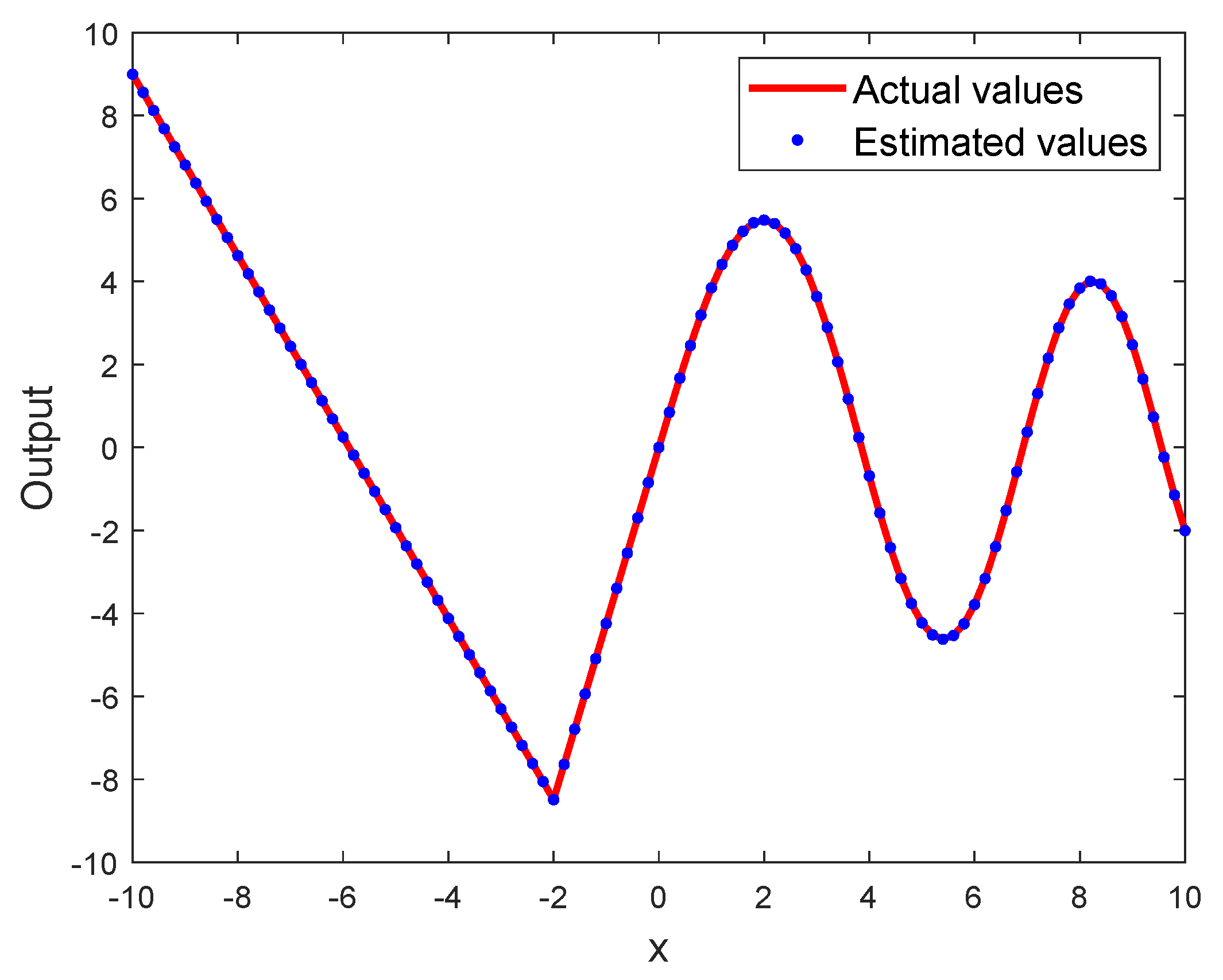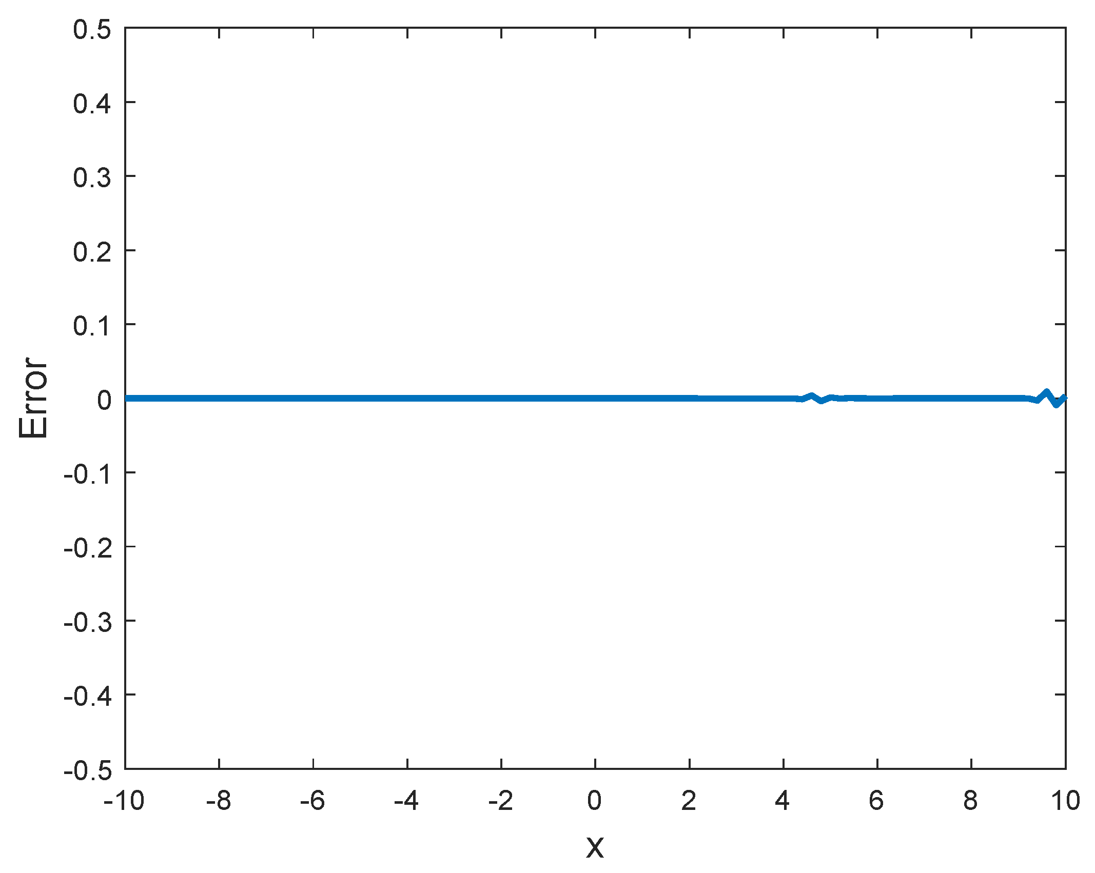Finally, Figure 4 demonstrates the strong approximation ability of LWNN, and Figure 5 describes the approximation error variation at the corresponding discrete data points of the function as follows.

In Figure 4, the solid line and dotted line denote the actual values and estimated values, respectively. As shown in Figure 5, good results are achieved using the proposed method.

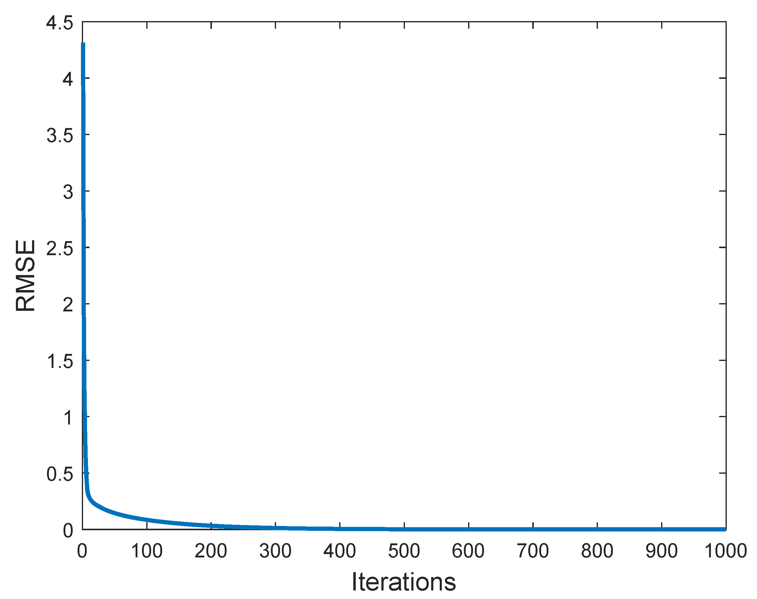
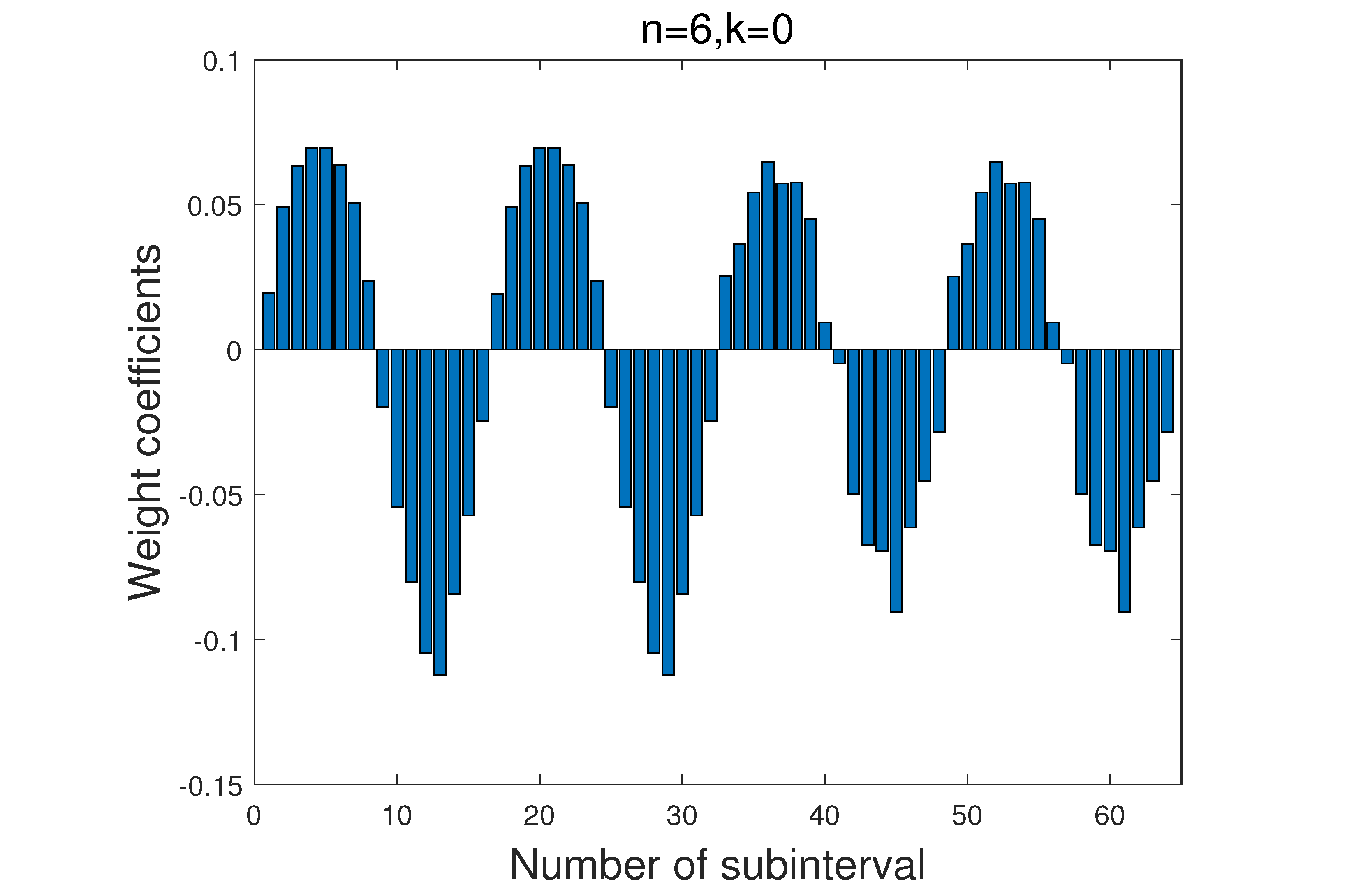
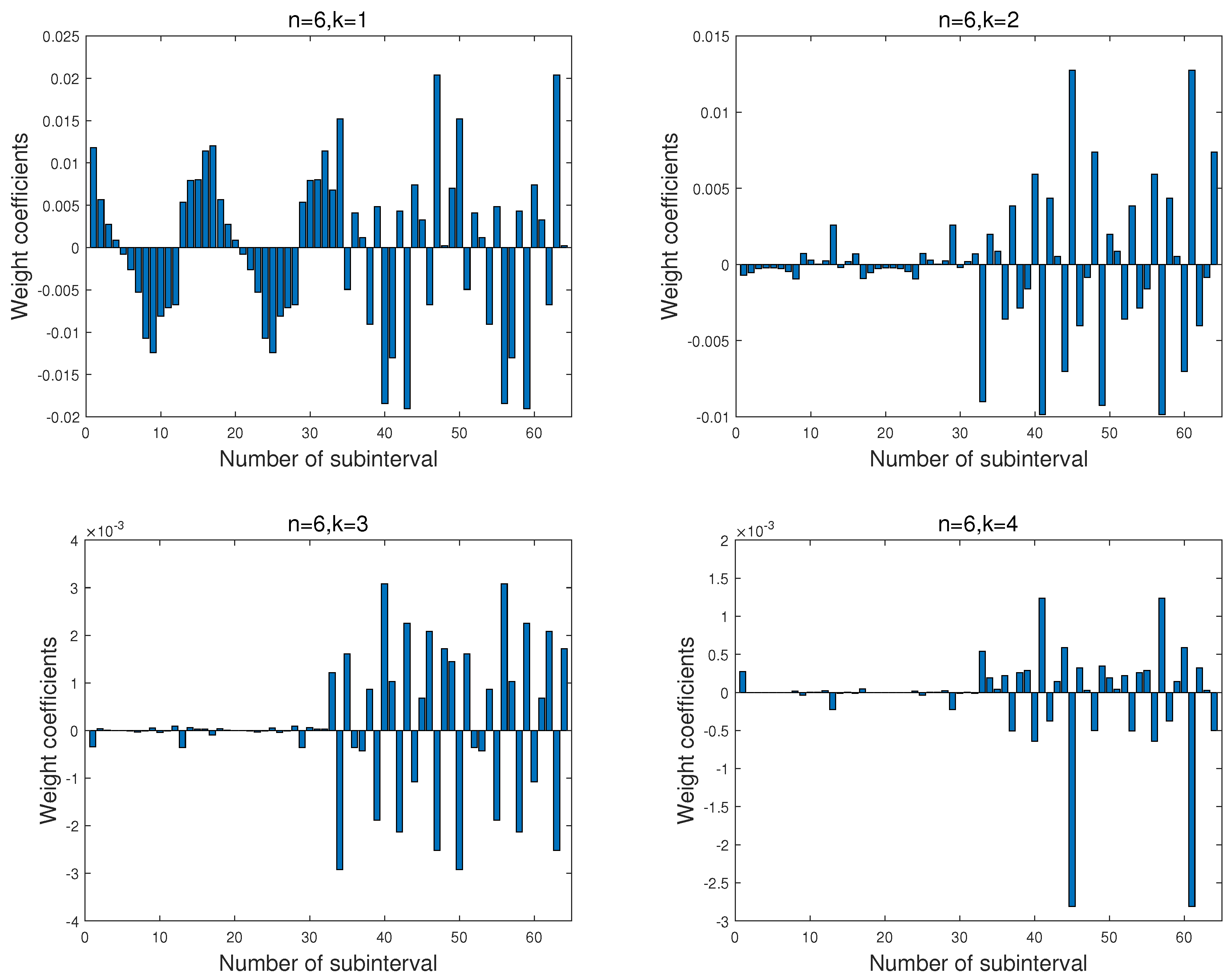
In addition, the RMSE iteration process of the proposed method is illustrated in Figure 6, and the learned network weight coefficients of the optimized structure are elaborately described in Figure 7, as follows.

As shown in Figure 7, the low-order LW bases approximate the trend of the function, and the high-order LW base functions learn the detailed features. The learned weight coefficients of LWNN record the non-derivable feature at the point $x=-2$ of the function on the 13th subinterval with the order $p=0$ and $p=1$, respectively. Especially, the weight coefficients of LWNN with the order $p=1$ demonstrate the step variation of the function.

Finally, other existing methods are compared to the proposed method, and

Table 3. The proposed method compared to other research results (Example 1).

Methods	Parameters	RMSE
WN [27]	22	0.0506
WNN [44]	107	0.0072
FWN [45]	26	0.0071
FWNN-GA [46]	20	0.0303
SLFRWNN [39]	18	0.0190
mPSOWIIR algorithm [47]	—	0.0182
Proposed method	32	0.0015

Note: The bold and highlighted text in the table represents the proposed method and its corresponding parameters and RMSE value.

shows the comparison results.

As described in Table 3, the proposed method provides the highest approximation accuracy compared to other existing methods.

4.2. Example 2

In this experiment, a nonlinear dynamical system studied by different existing methods and recognition models [36,38,39,48] is identified using the proposed method in this article. The corresponding dynamical system is described by the following difference equation

$$y\left(x\right)=0.72y(x-1)+0.025y(x-2)u(x-1)+0.01u^2(x-2)+0.2u(x-3).$$

(14)

As represented by (13), the current output of the system $y\left(x\right)$ depends on the system previous outputs $y(x-1),y(x-2)$ and the previous input $u(x-1),u(x-2),u(x-3)$. Correspondingly, the input $u\left(x\right)$ of this dynamical system is described by

$$u\left(x\right)=\left\{\begin{array}{cc}sin(\pi x/25),\hfill & 0\le x<250,\hfill \\ 1,\hfill & 250\le x<500,\hfill \\ -1,\hfill & 500\le x<750,\hfill \\ 0.3sin(\pi x/25)+0.1sin(\pi x/32)+0.6sin(\pi x/10),\hfill & 750\le x\le 1000.\hfill \end{array}\right.$$

(15)

Then, the training samples and testing samples of the proposed method are composed of the control variable x and the current output $y\left(x\right)$ values, which are the input–output sample point pairs for this dynamical system identification. By substituting the control variable data x into (14), the control sample data $u\left(x\right)$ are obtained and they are substituted into this system (13) to generate 1000 training and testing samples. Based on the generated samples, 800 samples are randomly selected as the training samples and the remaining samples are adopted as the testing samples. Finally, the identification results of this nonlinear dynamical system using the proposed method with different resolution level n and order p of LW bases are elaborately shown in

Table 4. Identification results with different resolution levels and orders (Example 2).

n	p	Training RMSE	Testing RMSE
4	6	0.0962	0.1030
4	7	0.0807	0.1010
4	8	0.0558	0.0849
5	6	0.00678	0.0132
5	7	0.00232	0.00639
5	8	0.00121	0.00375

as follows.

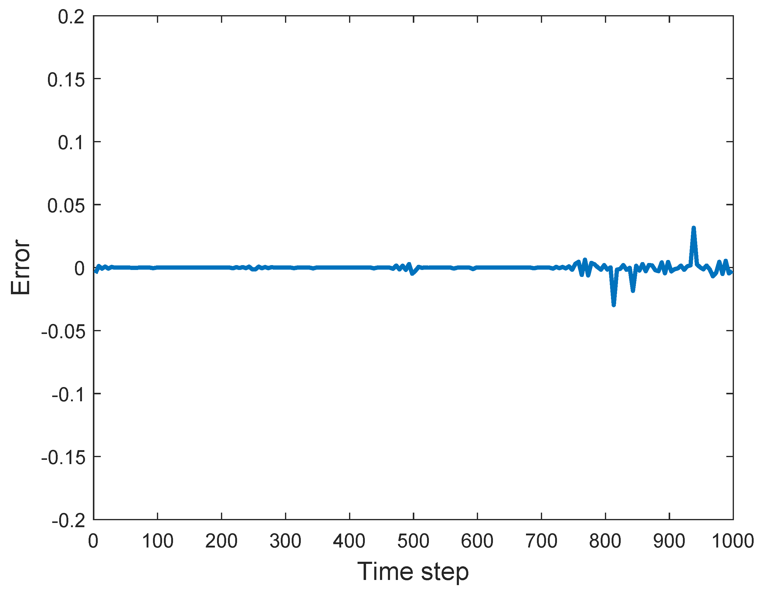
As described in Table 4, the resolution level $n=5$ and the order $p=8$ of LW bases are the optimal structure of LWNN. The optimal RMSE value of this example for the testing samples is $0.00375$. The good performance is described further by comparing the difference between the actual values (solid line) with the estimated values (dashed line) in Figure 8 and Figure 9, respectively.

Finally, the RMSE iteration process of training LWNN to identify this dynamical system, and the network weight coefficients learned by the improved gradient descent algorithm are shown in Figure 10 and Figure 11, respectively.

As demonstrated in Figure 11, the network weight coefficients with a different order of LW bases illustrate the strong ability of LWNN learning the essential features of this dynamical system. Specifically, LWNN with the order $p=0 ,p=1$ and $p=2$ has effectively learned the step feature at the points $x=250$ and $x=500$ of this complex dynamical system on the $8,9$ th and $16,17$ th subintervals, respectively. Correspondingly, the network weight coefficients of LWNN have a sudden variation in the positive and negative values at the step points. Similarly, the ramp feature at the point $x=750$ of this dynamical system is described by the network weight coefficients of LW bases with the order $p=0$ and $p=2$ on the $24,25$ th subintervals, respectively. Additionally, the comparison results with other existing methods are elaborately described in

Table 5. The proposed method compared to other existing results (Example 2).

Methods	Parameters	Training RMSE	Testing RMSE
MNN [49]	—	—	0.0668
RSONFIN [50]	49	0.030	0.06
TRFN-S [51]	33	0.0067	0.0313
FARNN [52]	—	—	0.000358
STFWN [53]	40	0.02	0.0042
FWNN [36]	43	0.0187	0.0202
FWNN-M [54]	32	0.0096	0.0213
WSVR-ADLA-WNNs [55]	—	—	0.0032
WSVR-FNN [55]	21	0.0101	0.0111
PRWNN [56]	52	—	0.0102
RWN [56]	48	—	0.0171
FWNN [38]	30	0.0067	0.0163
SLFRWNN [39]	33	0.0042	0.0076
WK-FNN [40]	—	0.00576	0.00598
Proposed method	32	0.00121	0.00376

Note: The bold and highlighted text in the table represents the proposed method and its corresponding parameters and RMSE value.

as follows.

From the obtained results in Table 5, the proposed method can significantly enhance the identification accuracy due to the main neurons in LWNN representation by the polynomials, which can provide the highest accuracy with the optimal control parameters of the network structure.

4.3. Example 3

In this example, the nonlinear dynamical system mentioned in Refs. [47,57,58] is represented by the following difference equation

$$y(x+1)=f\left[y\right(x),y(x-1),y(x-2),u(x),u(x-1\left)\right],$$

(16)

where the function f has the following form

$$f\left(x_1,x_2,x_3,x_4,x_5\right)=\frac{x_1{x}_2{x}_3{x}_5\left(x_3-1\right)+x_4}{1+x_3^2+x_2^2},$$

(17)

The input $u\left(x\right)$ of this dynamical system is described by

$$u\left(x\right)=\left\{\begin{array}{cc}sin(2\pi x/250),\hfill & 0\le x<500,\hfill \\ 0.8sin(2\pi x/250)+0.2sin(2\pi x/250),\hfill & 500\le x\le 1000.\hfill \end{array}\right.$$

(18)

The input–output data pairs of this dynamical system identification are still composed of the control variable x and the current output $y\left(x\right)$ of this dynamical system. Accordingly, 2000 samples are randomly generated by (15)–(17) and 1800 samples are used as training data and the rest of the samples as testing data. The simulation results of system identification with different decomposition scale n and order p of Legendre multiwavelet basis are illustrated in

Table 6. Identification results with different resolution levels and orders (Example 3).

n	p	Training RMSE	Testing RMSE
5	2	0.05228	0.05139
5	3	0.03088	0.03087
5	4	0.01290	0.01355
6	2	0.01154	0.01103
6	3	0.00503	0.00536
6	4	0.00175	0.00203

The optimal RMSE value of this dynamical system identification is $0.00203$, which can be found in Table 6 when the decomposition scale $n=6$ and order $p=5$ of Legendre multiwavelet basis. Additionally, Figure 12 and Figure 13 show that LWNN obtains a good response of this dynamical system, respectively.

Furthermore, the error iteration process of LWNN identification of this dynamical system and the network weight coefficients obtained are shown in Figure 14 and Figure 15, respectively.

In Figure 15, the obtained network weight coefficients describe the ability of LWNN learning the feature of this dynamical system. When $x\ge 500$, the impulse signal presented by this dynamical system becomes more complicated. Then, LWNN with the order $p=0$ of Legendre multiwavelet basis records the main tread characteristic of this dynamical system, and LWNN with the order $p\ge 2$ of LW bases effectively learns this complex impulse signal feature from $32\mathrm{th}$ to $64\mathrm{th}$ subintervals.

In contrast to the other methods,

Table 7. The proposed method compared to other research results (Example 3).

Methods	Parameters	Training RMSE	Testing RMSE
NN [57]	—	—	—
FWNN [58]	—	—	0.0406
FLANN-PSO [59]	—	—	0.0052
mPSOWIIR algorithm [47]	—	—	0.000066176
Proposed method	64	0.00175	0.00203

shows the comparison results.

From the obtained results in Table 7, LWNN can provide better accuracy in identifying this dynamical system.

4.4. Example 4

In this experiment, a second-order nonlinear dynamical system studied by various models [33,36,37,54] is identified using the proposed LWNN-GA method. The difference equation of this dynamical system and the function f is represented using (15) and (16) in Example 3. The corresponding control signal $u\left(x\right)$ of this complex dynamical system is demonstrated using (14). Then, 2500 data samples randomly generated using (14), (15), and (16) are applied to identify this second-order nonlinear dynamical system by using LWNN. Accordingly, 2000 data samples are used as training data and 500 data samples are used as testing data, respectively. The simulation results of this second-order nonlinear system identification with different decomposition scale n and order p of Legendre multiwavelet basis are described in

Table 8. Simulation results with different resolution levels and orders (Example 4).

n	p	Training RMSE	Testing RMSE
5	7	0.0368	0.0371
5	8	0.0320	0.0327
5	9	0.0287	0.0284
6	6	0.0252	0.0234
6	7	0.0215	0.0175
6	8	0.0179	0.0161

.

As described in Table 8, the optimal RMSE value obtained is $0.0161$ which attains the optimal resolution level $n=6$ and order $p=8$ of LW bases. Furthermore, Figure 16 and Figure 17 demonstrate that the proposed method obtains a good response of this complex dynamical system identification, respectively.

From the obtained results, it can be seen that LWNN has good performance for identification of this complex dynamical system. Then, the error iteration process of LWNN identification of this dynamical system and the network weight coefficients are shown in Figure 18 and Figure 19, respectively.

From the variation values of the network weight coefficients described in Figure 19, the proposed method has the ability of thoroughly learning the complex features of this dynamical system, such as uncertainties, step, ramp, and nonlinear. The main reason is that LW bases have rich properties such as compact support, orthogonality, vanishing moments, and especially various regularities, which can effectively approximate the nonlinear dynamical system. Specifically, the optimal structure of LWNN with the order from $p=0$ to $p=3$ of LW bases effectively learns the main tread feature of this complex dynamical system. Correspondingly, the optimal structure of LWNN with the order $p>3$ of LW bases still demonstrates the step and ramp characteristics at the points $x=250,500,700$ of this complex dynamical system. The learned network weight coefficients describe the trend on the $16,17$ th, $32,33$ th and $48,49$ th subintervals, respectively.

Additionally,

Table 9. Comparison of the proposed method with the existing methods (Example 4).

Methods	Parameters	Training RMSE	Testing RMSE
MNN [49]	—	—	0.0186
TRFN-S [48]	33	0.0084	0.0346
FWNN [36]	27	0.0292	0.0312
T1TSKFNS [60]	63	0.0282	0.0598
FWNN-S [54]	32	0.0209	0.0337
FWNN-M [54]	32	0.0193	0.0333
PRWNN [56]	52	—	0.0301
RWNN [56]	48	—	0.0328
FWNN [38]	30	0.0202	0.0274
eIT2FNN-LSTM [33]	72	0.0237	0.0283
LWNN	64	0.0179	0.0161

Note: The bold and highlighted text in the table represents the proposed method and its corresponding parameters and RMSE value.

shows the comparison results with the other methods as follows.

To summarize, according to the results obtained in the above four examples, the identification accuracy shown in Table 2, Table 4, Table 6, Table 8, and Table 9 using the proposed method is basically consistent with the approximation error in (4). Furthermore, as described in Figure 6, Figure 10, Figure 14, and Figure 18, the proposed method effectively decrease the learning iteration steps by combing the simple Genetic Algorithm with the improved gradient descent algorithm in the nonlinear dynamical system identification. Correspondingly, the learned network weight coefficients of LWNN with the optimal structure can describe the complex features of the dynamical systems as shown in Figure 7, Figure 11, Figure 15, and Figure 19. Therefore, the proposed method demonstrates good performance and generalization ability for the identification of various complex dynamical systems.

5. Conclusions

In this paper, the two control parameters of LWNN structure are optimized using the simple Genetic Algorithm. Then, the weight coefficients of the optimal network are learned using the improved gradient descent algorithm, which are effectively implemented to identify four nonlinear dynamical systems. The simple Genetic Algorithm is utilized to find the appropriate LW bases in the hidden layer of LWNN, and avoid the complex calculations of the translation and dilation parameters of the traditional WNN. In addition, better identification accuracy of the nonlinear dynamic system is obtained with the optimal network structure. In future research, the proposed method should combine the advantage of the RNN model with a feed forward network and feedback loop to devise more effective LWNNs with a feedback loop. These enhanched models could then be implemented to identify the nonlinear dynamical system in application fields,. Additionally, the approach should be expanded to construct multidimensional LWNNs and study their implementation in various applications.

References

1. Jin, L.; Liu, Z.; Li, L. Prediction and identification of nonlinear dynamical systems using machine learning approaches. J. Ind. Inf. Integr. 2023, 35, 100503. [Google Scholar] [CrossRef]
2. Cheng, A.; Low, Y.M. Improved generalization of NARX neural networks for enhanced metamodeling of nonlinear dynamic systems under stochastic excitations. Mech. Syst. Signal Process. 2023, 200, 110543. [Google Scholar] [CrossRef]
3. Quaranta, G.; Lacarbonara, W.; Masri, S.F. A review on computational intelligence for identification of nonlinear dynamical systems. Nonlinear Dyn. 2020, 99, 1709–1761. [Google Scholar] [CrossRef]
4. Truong, H.V.A.; Nguyen, M.H.; Tran, D.T.; Ahn, K.K. A novel adaptive neural network-based time-delayed estimation control for nonlinear systems subject to disturbances and unknown dynamics. ISA Trans. 2023, 142, 214–227. [Google Scholar] [CrossRef]
5. Brewick, P.T.; Masri, S.F. An evaluation of data-driven identification strategies for complex nonlinear dynamic systems. Nonlinear Dyn. 2016, 85, 1297–1318. [Google Scholar] [CrossRef]
6. Chen, H.; Liu, Z.; Alippi, C.; Huang, B.; Liu, D. Explainable intelligent fault diagnosis for nonlinear dynamic systems: From unsupervised to supervised learning. IEEE Trans. Neural. Netw. Learn. Syst. 2022, 1–14. [Google Scholar] [CrossRef] [PubMed]
7. Chen, H.; Li, L.; Shang, C.; Huang, B. Fault detection for nonlinear dynamic systems with consideration of modeling errors: A data-driven approach. IEEE Trans. Cybern. 2022. [Google Scholar] [CrossRef] [PubMed]
8. Chu, Y.; Fei, J.; Hou, S. Adaptive global sliding-mode control for dynamic systems using double hidden layer recurrent neural network structure. IEEE Trans. Neural Netw. Learn. Syst. 2019, 31, 1297–1309. [Google Scholar] [CrossRef]
9. Revay, M.; Wang, R.; Manchester, I.R. Recurrent equilibrium networks: Flexible dynamic models with guaranteed stability and robustness. IEEE Trans. Autom. Control. 2023. [Google Scholar] [CrossRef]
10. Otto, S.E.; Rowley, C.W. Linearly recurrent autoencoder networks for learning dynamics. SIAM J. Appl. Dyn. Syst. 2019, 18, 558–593. [Google Scholar] [CrossRef]
11. de Campos Souza, P.V. Fuzzy neural networks and neuro-fuzzy networks: A review the main techniques and applications used in the literature. Appl. Soft Comput. 2020, 92, 106275. [Google Scholar] [CrossRef]
12. Fei, J.; Liu, L. Real-time nonlinear model predictive control of active power filter using self-feedback recurrent fuzzy neural network estimator. IEEE Trans. Ind. Electron. 2021, 69, 8366–8376. [Google Scholar] [CrossRef]
13. Wu, X.; Han, H.; Liu, Z.; Qiao, J. Data-knowledge-based fuzzy neural network for nonlinear system identification. IEEE Trans. Fuzzy Syst. 2019, 28, 2209–2221. [Google Scholar] [CrossRef]
14. Ribeiro, G.T.; Mariani, V.C.; dos Santos Coelho, L. Enhanced ensemble structures using wavelet neural networks applied to short-term load forecasting. Eng. Appl. Artif. Intell. 2019, 82, 272–281. [Google Scholar] [CrossRef]
15. Jin, M.; Brake, M.R.; Song, H. Comparison of nonlinear system identification methods for free decay measurements with application to jointed structures. J. Sound Vib. 2019, 453, 268–293. [Google Scholar] [CrossRef]
16. Luo, G.; Yang, Z.; Zhang, Q. Identification of autonomous nonlinear dynamical system based on discrete-time multiscale wavelet neural network. Neural Comput. Appl. 2021, 33, 15191–15203. [Google Scholar] [CrossRef]
17. Hamedani, M.H.; Zekri, M.; Sheikholeslam, F.; Selvaggio, M.; Ficuciello, F.; Siciliano, B. Recurrent fuzzy wavelet neural network variable impedance control of robotic manipulators with fuzzy gain dynamic surface in an unknown varied environment. Fuzzy Sets Syst. 2021, 416, 1–26. [Google Scholar] [CrossRef]
18. Sheikhlar, Z.; Hedayati, M.; Tafti, A.D.; Farahani, H.F. Fuzzy Elman Wavelet Network: Applications to function approximation, system identification, and power system control. Inf. Sci. 2022, 583, 306–331. [Google Scholar] [CrossRef]
19. Kumar, R. Memory recurrent Elman neural network-based identification of time-delayed nonlinear dynamical system. IEEE Trans. Syst. Man Cybern. Syst. 2022, 53, 753–762. [Google Scholar] [CrossRef]
20. Luo, S.; Lewis, F.L.; Song, Y.; Garrappa, R. Dynamical analysis and accelerated optimal stabilization of the fractional-order self-sustained electromechanical seismograph system with fuzzy wavelet neural network. Nonlinear Dyn. 2021, 104, 1389–1404. [Google Scholar] [CrossRef]
21. Sharifi, A.; Sharafian, A.; Ai, Q. Adaptive MLP neural network controller for consensus tracking of Multi-Agent systems with application to synchronous generators. Expert Syst. Appl. 2021, 184, 115460. [Google Scholar] [CrossRef]
22. Bukhari, A.H.; Raja, M.A.Z.; Rafiq, N.; Shoaib, M.; Kiani, A.K.; Shu, C.M. Design of intelligent computing networks for nonlinear chaotic fractional Rossler system. Chaos Solitons Fractals 2022, 157, 111985. [Google Scholar] [CrossRef]
23. Fei, J.; Lu, C. Adaptive sliding mode control of dynamic systems using double loop recurrent neural network structure. IEEE Trans. Neural Netw.Learn. Syst. 2017, 29, 1275–1286. [Google Scholar] [CrossRef] [PubMed]
24. Moradi Ghahderijani, M.; Castilla, M.; Momeneh, A.; Miret, J.; Garcia de Vicuna, L. Robust and Fast sliding-mode control for a DC–DC current-source parallel-resonant converter. IET Power Electron. 2018, 11, 262–271. [Google Scholar] [CrossRef]
25. Zeng, W.; Li, M.; Yuan, C.; Wang, Q.; Liu, F.; Wang, Y. Identification of epileptic seizures in EEG signals using time-scale decomposition (ITD), discrete wavelet transform (DWT), phase space reconstruction (PSR) and neural networks. Artif. Intell. Rev. 2020, 53, 3059–3088. [Google Scholar] [CrossRef]
26. Kumar, R.; Srivastava, S.; Gupta, J.; Mohindru, A. Comparative study of neural networks for dynamic nonlinear systems identification. Soft Comput. 2019, 23, 101–114. [Google Scholar] [CrossRef]
27. Zhang, Q.; Benveniste, A. Wavelet networks. IEEE Trans. Neural Netw. 1992, 3, 889–898. [Google Scholar] [CrossRef]
28. Alexandridis, A.K.; Zapranis, A.D. Wavelet neural networks: A practical guide. Neural Netw. 2013, 42, 1–27. [Google Scholar] [CrossRef]
29. Guo, T.; Zhang, T.; Lim, E.; Lopez-Benitez, M.; Ma, F.; Yu, L. A review of wavelet analysis and its applications: Challenges and opportunities. IEEE Access 2022, 10, 58869–58903. [Google Scholar] [CrossRef]
30. Ko, C.N. Identification of nonlinear systems with outliers using wavelet neural networks based on annealing dynamical learning algorithm. Eng. Appl. Artif. Intell. 2012, 25, 533–543. [Google Scholar] [CrossRef]
31. Yoo, S.J.; Park, J.B.; Choi, Y.H. Indirect adaptive control of nonlinear dynamic systems using self recurrent wavelet neural networks via adaptive learning rates. Inf. Sci. 2007, 177, 3074–3098. [Google Scholar] [CrossRef]
32. Zainuddin, Z.; Pauline, O. Modified wavelet neural network in function approximation and its application in prediction of time-series pollution data. Appl. Soft Comput. 2011, 11, 4866–4874. [Google Scholar] [CrossRef]
33. Samanta, S.; Suresh, S.; Senthilnath, J.; Sundararajan, N. A new neuro-fuzzy inference system with dynamic neurons (nfis-dn) for system identification and time series forecasting. Appl. Soft Comput. 2019, 82, 105567. [Google Scholar] [CrossRef]
34. Emami, S.A.; Roudbari, A. Identification of nonlinear time-varying systems using wavelet neural networks. Adv. Control Appl. Eng. Ind. Syst. 2020, 2, e59. [Google Scholar] [CrossRef]
35. Davanipoor, M.; Zekri, M.; Sheikholeslam, F. Fuzzy wavelet neural network with an accelerated hybrid learning algorithm. IEEE Trans. Fuzzy Syst. 2011, 20, 463–470. [Google Scholar] [CrossRef]
36. Abiyev, R.H.; Kaynak, O. Fuzzy wavelet neural networks for identification and control of dynamic plants—A novel structure and a comparative study. IEEE Trans. Ind. Electron. 2008, 55, 3133–3140. [Google Scholar] [CrossRef]
37. Wang, H.; Luo, C.; Wang, X. Synchronization and identification of nonlinear systems by using a novel self-evolving interval type-2 fuzzy LSTM-neural network. Eng. Appl. Artif. Intell. 2019, 81, 79–93. [Google Scholar] [CrossRef]
38. Cheng, R.; Bai, Y. A novel approach to fuzzy wavelet neural network modeling and optimization. Int. J. Electr. Power Energy Syst. 2015, 64, 671–678. [Google Scholar] [CrossRef]
39. Ganjefar, S.; Tofighi, M. Single-hidden-layer fuzzy recurrent wavelet neural network: Applications to function approximation and system identification. Inf. Sci. 2015, 294, 269–285. [Google Scholar] [CrossRef]
40. Loussifi, H.; Nouri, K.; Braiek, N.B. A new efficient hybrid intelligent method for nonlinear dynamical systems identification: The Wavelet Kernel Fuzzy Neural Network. Commun. Nonlinear Sci. Numer. Simul. 2016, 32, 10–30. [Google Scholar] [CrossRef]
41. Alpert, B.K. A class of bases in L2 for the sparse representation of integral operators. SIAM J. Math. Anal. 1993, 24, 246–262. [Google Scholar] [CrossRef]
42. Alpert, B.; Beylkin, G.; Gines, D.; Vozovoi, L. Adaptive solution of partial differential equations in multiwavelet bases. J. Comput. Phys. 2002, 182, 149–190. [Google Scholar] [CrossRef]
43. Ling, S.H.; Iu, H.H.C.; Leung, F.H.F.; Chan, K.Y. Improved hybrid particle swarm optimized wavelet neural network for modeling the development of fluid dispensing for electronic packaging. IEEE Trans. Ind. Electron. 2008, 55, 3447–3460. [Google Scholar] [CrossRef]
44. Safavi, A.; Romagnoli, J. Application of wavelet-based neural networks to the modelling and optimisation of an experimental distillation column. Eng. Appl. Artif. Intell. 1997, 10, 301–313. [Google Scholar] [CrossRef]
45. Ebadat, A.; Noroozi, N.; Safavi, A.A.; Mousavi, S.H. New fuzzy wavelet network for modeling and control: The modeling approach. Commun. Nonlinear Sci. Numer. Simul. 2011, 16, 3385–3396. [Google Scholar] [CrossRef]
46. Tzeng, S.T. Design of fuzzy wavelet neural networks using the GA approach for function approximation and system identification. Fuzzy Sets Syst. 2010, 161, 2585–2596. [Google Scholar] [CrossRef]
47. Carrillo-Santos, C.; Seck-Tuoh-Mora, J.; Hernandez-Romero, N.; Ramos-Velasco, L. Wavenet identification of dynamical systems by a modified PSO algorithm. Eng. Appl. Artif. Intell. 2018, 73, 1–9. [Google Scholar] [CrossRef]
48. Juang, C.F. A TSK-type recurrent fuzzy network for dynamic systems processing by neural network and genetic algorithms. IEEE Trans. Fuzzy Syst. 2002, 10, 155–170. [Google Scholar] [CrossRef]
49. Sastry, P.; Santharam, G.; Unnikrishnan, K. Memory neuron networks for identification and control of dynamical systems. IEEE Trans. Neural Netw. 1994, 5, 306–319. [Google Scholar] [CrossRef]
50. Gough, J. Asymptotic stochastic transformations for nonlinear quantum dynamical systems. Rep. Math. Phys. 1999, 44, 313–338. [Google Scholar] [CrossRef]
51. Juang, C.F.; Lin, C.T. A recurrent self-organizing neural fuzzy inference network. IEEE Trans. Neural Netw. 1999, 10, 828–845. [Google Scholar] [CrossRef]
52. Wang, J.S.; Chen, Y.P. A fully automated recurrent neural network for unknown dynamic system identification and control. IEEE Trans. Circuits Syst. I Regul. Pap. 2006, 53, 1363–1372. [Google Scholar] [CrossRef]
53. Juang, C.F.; Chiou, C.T.; Lai, C.L. Hierarchical singleton-type recurrent neural fuzzy networks for noisy speech recognition. IEEE Trans. Neural Netw. 2007, 18, 833–843. [Google Scholar] [CrossRef] [PubMed]
54. Yilmaz, S.; Oysal, Y. Fuzzy wavelet neural network models for prediction and identification of dynamical systems. IEEE Trans. Neural Netw. 2010, 21, 1599–1609. [Google Scholar] [CrossRef] [PubMed]
55. Ko, C.N. WSVR-based fuzzy neural network with annealing robust algorithm for system identification. J. Frankl. Inst. 2012, 349, 1758–1780. [Google Scholar] [CrossRef]
56. Zhao, H.; Gao, S.; He, Z.; Zeng, X.; Jin, W.; Li, T. Identification of nonlinear dynamic system using a novel recurrent wavelet neural network based on the pipelined architecture. IEEE Trans. Ind. Electron. 2013, 61, 4171–4182. [Google Scholar] [CrossRef]
57. Kumpati, S.N.; Kannan, P. Identification and control of dynamical systems using neural networks. IEEE Trans. Neural Netw. 1990, 1, 4–27. [Google Scholar]
58. Ho, D.W.; Zhang, P.A.; Xu, J. Fuzzy wavelet networks for function learning. IEEE Trans. Fuzzy Syst. 2001, 9, 200–211. [Google Scholar] [CrossRef]
59. Majhi, B.; Panda, G. Development of efficient identification scheme for nonlinear dynamic systems using swarm intelligence techniques. Expert Syst. Appl. 2010, 37, 556–566. [Google Scholar] [CrossRef]
60. Abiyev, R.H.; Kaynak, O. Type 2 fuzzy neural structure for identification and control of time-varying plants. IEEE Trans. Ind. Electron. 2010, 57, 4147–4159. [Google Scholar] [CrossRef]
Figure 1. The structure of LWNN.
Mathematics 11 04913 g001
Figure 2. The structure of the main neuron ϕ k , n l in the hidden layer of LWNN.
Mathematics 11 04913 g002
Figure 3. The flowchart of the proposed method for nonlinear system identification.
Mathematics 11 04913 g003
Figure 4. Comparison of the actual values and the estimated values (Example 1).
Mathematics 11 04913 g004
Figure 5. Error between the actual values and the estimated values (Example 1).
Mathematics 11 04913 g005
Figure 6. RMSE varies with the iterations (Example 1).
Mathematics 11 04913 g006
Figure 7. Learned network weight coefficients using the proposed method (Example 1).
Mathematics 11 04913 g007aMathematics 11 04913 g007b
Figure 8. Comparison of the actual values and the estimated values (Example 2).
Mathematics 11 04913 g008
Figure 9. Error between the actual values and the estimated values (Example 2).
Mathematics 11 04913 g009
Figure 10. Illustration of how RMSE varies with the iterations (Example 2).
Mathematics 11 04913 g010
Figure 11. Learned network weight coefficients using the proposed method (Example 2).
Mathematics 11 04913 g011
Figure 12. Comparison of the actual values and the estimated values (Example 3).
Mathematics 11 04913 g012
Figure 13. Error between the actual values and the estimated values (Example 3).
Mathematics 11 04913 g013
Figure 14. Illustration of how RMSE varies with the iterations (Example 3).
Mathematics 11 04913 g014
Figure 15. Network weight coefficients with the optimal control parameters by LWNN (Example 3).
Mathematics 11 04913 g015aMathematics 11 04913 g015b
Figure 16. Comparison of the actual values and the estimated values (Example 4).
Mathematics 11 04913 g016
Figure 17. Error between the actual values and the estimated values (Example 4).
Mathematics 11 04913 g017
Figure 18. RMSE varies with the iterations (Example 4).
Mathematics 11 04913 g018
Figure 19. Network weight coefficients with the optimal control parameters of LWNN (Example 4).
Mathematics 11 04913 g019