Article

Using a Node–Child Matrix to Address the Quickest Path Problem in Multistate Flow Networks under Transmission Cost Constraints

by
Majid Forghani-elahabad
1,* and
Omar Mutab Alsalami
2
1
Center of Mathematics, Computing, and Cognition, Federal University of ABC, Santo André 09210-580, SP, Brazil
2
Department of Electrical Engineering, College of Engineering, Taif University, P.O. Box 11099, Taif 21944, Saudi Arabia
*
Author to whom correspondence should be addressed.
Mathematics 2023, 11(24), 4889; https://doi.org/10.3390/math11244889
Submission received: 9 November 2023 / Revised: 1 December 2023 / Accepted: 4 December 2023 / Published: 6 December 2023
(This article belongs to the Special Issue Graph Theory and Network Theory)

Abstract

:
The quickest path problem in multistate flow networks, which is also known as the quickest path reliability problem (QPRP), aims at calculating the probability of successfully sending a minimum of d flow units/data/commodity from a source node to a destination node via one minimal path (MP) within a specified time frame of T units. Several exact and approximative algorithms have been proposed in the literature to address this problem. Most of the exact algorithms in the literature need prior knowledge of all of the network’s minimal paths (MPs), which is considered a weak point. In addition to the time, the budget is always limited in real-world systems, making it an essential consideration in the analysis of systems’ performance. Hence, this study considers the QPRP under cost constraints and provides an efficient approach based on a node–child matrix to address the problem without knowing the MPs. We show the correctness of the algorithm, compute the complexity results, illustrate it through a benchmark example, and describe our extensive experimental results on one thousand randomly generated test problems and well-established benchmarks to showcase its practical superiority over the available algorithms in the literature.

1. Introduction

The quickest path problem involves identifying a path from a source node, 1, to a destination node, n, within a network. This path is used to efficiently transmit a specific flow quantity, d, from node one to node n while minimizing the transmission time [1,2]. In this problem, each network arc is characterized by two key attributes: a lead time value and a capacity value. The significance of this optimization problem is well recognized by researchers due to its applicability across a broad spectrum of flow network scenarios [1,2,3,4,5,6,7,8,9,10,11,12,13]. This problem initially emerged when discovering the fastest route for convoy-type traffic within flow-rate-constrained networks [1]. Subsequently, it found application in communication networks, where nodes represent transmitters/receivers and arcs symbolize communication channels [2].
While deterministic (non-stochastic) flow networks have undeniably been instrumental in understanding and optimizing various systems, the practical reality is that many real-world systems exhibit dynamic characteristics, necessitating the adoption of a more nuanced approach. Multistate (stochastic) flow networks (MFNs) have gained prominence as a result of their ability to model complex systems in which fluctuations, failures, maintenance, and other dynamic factors play a significant role [14,15,16,17,18,19,20]. Within an MFN, arcs and nodes can exist in various potential states that are influenced by traffic conditions, maintenance activities, failures, or other underlying causes. Consequently, the network itself assumes multiple states, each reflecting the dynamic nature of the system. Numerous performance metrics have been introduced in the literature to evaluate the effectiveness of an MFN, with particular emphasis on network reliability, which stands out as a primary indicator. Network reliability is commonly defined as the system’s capacity to fulfill a predefined function within specified conditions and within a known time frame [21]. A well-known reliability indicator is the two-terminal reliability of an MFN. It is the probability of transmitting at least a given demand for d units of flow/data/commodity from node one (source) to node n (destination). Numerous exact and approximative algorithms have been proposed in the literature to compute this indicator [8,10,15,20,22,23,24,25,26,27,28,29,30,31,32,33,34].
Due to the inherent random variability in arc capacities within MFNs, the transmission time likewise exhibits stochastic behavior. In light of this uncertainty, the classical quickest path problem has evolved into a more comprehensive challenge known as the quickest path reliability problem (QPRP) within the context of MFNs [4,5,24,35,36,37,38]. The primary objective of the QPRP is to ascertain the probability of successfully transmitting a minimum of d units of flow from source node one to the destination node n via a single path, all while adhering to a stipulated time constraint of T units. This extension of the problem accounts for the dynamic and unpredictable nature of network conditions, making it particularly relevant in scenarios where both speed and reliability are paramount, such as in telecommunications, transportation, and various other domains [4,24,35,39,40].
Lin [35] introduced an algorithm that required all of the MPs as input. It determines the minimum capacity required for each MP to meet the time constraints for transmitting d flow units. Subsequently, by systematically evaluating each MP, the algorithm derives the solutions to the problem. Yeh et al. [39] harnessed the kth shortest path approach to devise an algorithm for addressing the problem. In subsequent work [40], they further refined and enhanced their algorithm. The QPRP was expanded to encompass scenarios involving two disjoint MPs in [37,41], as well as situations with multiple disjoint MPs in [37]. In a different approach, the researchers in [42] considered both time and budget constraints, and they utilized these constraints to efficiently reduce the computational complexity. Their extensive numerical analysis underscored the effectiveness of the proposed algorithm. Furthermore, the researchers in [5] recognized the computational limitations of the algorithm presented in [35]—mainly, when the network configuration involved over thirty relevant MPs. To address this challenge, they introduced an unbiased Monte Carlo estimator as an alternative to exact evaluation, offering a more scalable solution for large-scale scenarios. In a recent development that was detailed in [4], the authors addressed integrating budget constraints into the QPRP. They introduced an innovative approach that capitalized on budget and time constraints to streamline the process by eliminating redundant MPs before the execution of the algorithm. The authors then conducted extensive numerical experiments to underscore the enhanced performance of their approach when compared to existing methods in the literature. However, their algorithm still needs all of the MPs as input.
Recognizing the inherent computational challenge of determining all MPs, which is an N P —hard problem [43,44,45,46], this study introduces an efficient approach designed to address the QPRP under cost constraints without prior knowledge of MPs. Based on a node–child matrix, our proposed algorithm offers a novel methodology for solving the problem. To underscore its efficiency, we provide complexity analyses and present a wealth of experimental results, thus establishing the algorithm’s superior performance compared to existing methods in the literature.
The subsequent sections of this paper are structured as follows. Section 2 introduces the necessary notations, nomenclature, and assumptions. Section 3 presents some preliminary information about the problem. We propose the algorithm in Section 4. The complexity results, and an illustrative example are given in Section 5. In Section 6, we provide several numerical results on benchmarks and randomly generated test problems. Finally, Section 7 summarizes the work’s conclusions.

2. Notations, Nomenclature, and Assumptions
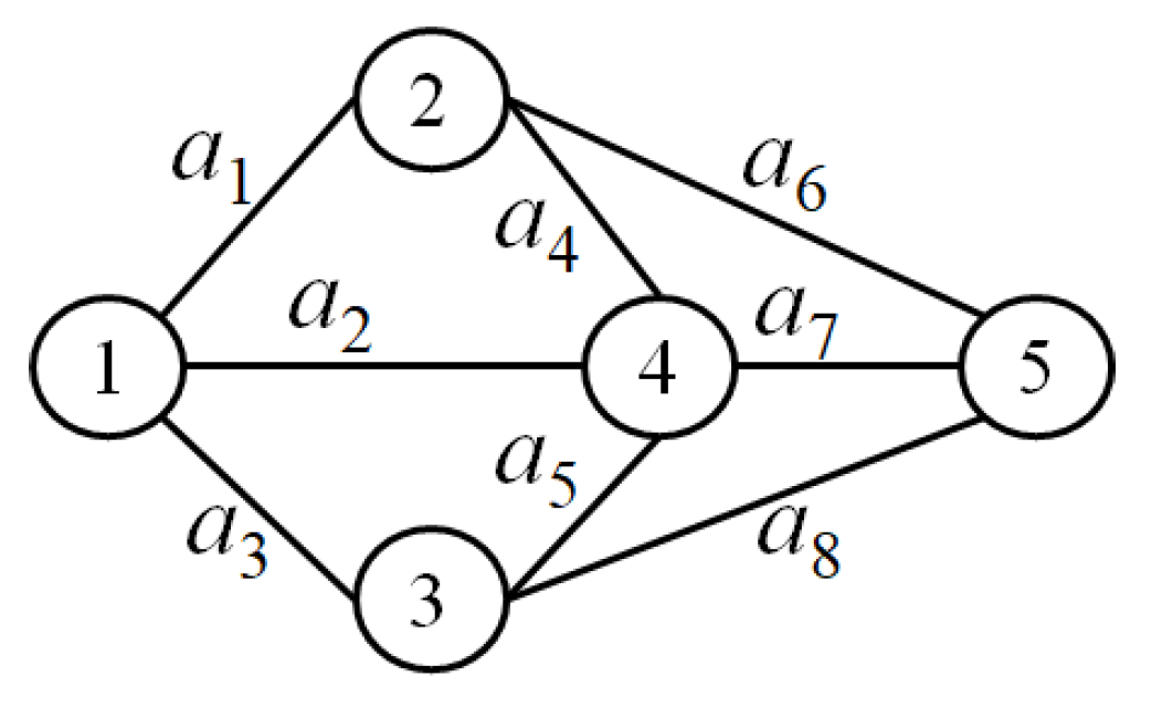
G G ( N , A , M , L , C ) represents a Multistate Flow Network (MFN), with N = { 1 , 2 , , n } as the node-set, where n signifies the total number of nodes. The collection of arcs is represented as A = { a 1 , a 2 , , a m } , where m corresponds to the number of arcs.
The MFN is further characterized by: (1)  M = ( M 1 , , M m ) , a maximum capacity vector, where M i signifies the max-capacity of arc a i for 1 i m . (2)  L = ( l 1 , , l m ) , a lead time vector, with each l i representing the lead time of arc a i for 1 i m . (3)  C = ( c 1 , , c m ) , a cost vector in which c i designates the transmission cost of arc a i for transmitting each unit of flow, for i = 1 , , m . Moreover, nodes 1 and n are considered respectively the source and destination nodes.
To illustrate, Figure 1 depicts an MFN defined by nodes’ set of N = { 1 , , 5 } and arcs’ set of A = { a 1 , , a 9 } . As an example, the network has lead time, maximum capacity, and cost vectors respectively as follows: L = ( 3, 1, 2, 3, 4, 3, 2, 3), M = ( 4, 2, 5, 4, 3, 3, 4, 5), and C = ( 2, 3, 4, 3, 2, 3, 2, 1). Consequently, for instance, the values within these vectors indicate that at most four units of flow can be transmitted concurrently at any time through a 1 , a 4 , or a 7 due to M 1 = M 4 = M 7 = 4 . Likewise, for example, l 8 = 3 denotes that passing up to M 8 = 5 units of flow through a 8 lasts three units of time. Furthermore, c 2 = 3 signifies that transmitting any flow unit on a 2 incurs a cost of three currency units.
X X = ( x 1 , x 2 , , x m ) represents the current system state vector (SSV). Here, 0 x i M i is an integer value, indicating the current capacity of arc a i for 1 i m . For instance, X = ( 3, 2, 3, 4, 3, 3, 3, 5) can be considered as a SSV for Figure 1.
I i shows the number of arcs incoming into node i for i = 1 , 2 , , n . We call this number the in-degree of the respective node. It is noted that I 1 = 0 because all flows originate from source node one, and no flow goes to the source node.
For instance, we have I 1 = 0 , I 2 = I 3 = I 5 = 3 , and I 4 = 4 in the network depicted in Figure 1.
O i represents the count of outgoing arcs from node i, where 1 i n . We call this the out-degree of the respective node. It is noted that O n = 0 because all flows go to the destination node, and no flow goes out of this node.
For instance, we have O 1 = O 4 = 3 , O 2 = O 3 = 2 , and O 5 = 0 in the network depicted in Figure 1.
P j is the jth minimal path (MP) for j = 1 , , h . So, h is the number of MPs in the network. As an example, P 1 = { a 1 , a 4 , a 5 , a 8 } represents an MP for the illustrated network in Figure 1.
K P j ( X ) K P j ( X ) = min { x i | a i P j } is the capacity of P j under SSV X for j = 1 , 2 , , h .
For instance, in Figure 1, the capacity of P 1 = { a 1 , a 4 , a 5 , a 8 } with X = ( 3, 2, 3, 4, 3, 3, 3, 5) is equal to K P 1 ( X ) = min { 3, 4, 3, 5 } = 3.
L P j L P j = i : a i P j l i is the lead time of the MP P j for j = 1, 2, , h . For instance, considering L = ( 3, 1, 2, 3, 4, 3, 2, 3), we have L P 1 = l 1 + l 4 + l 5 + l 8 = 13 for P 1 = { a 1 , a 4 , a 5 , a 8 } .
C P j C P j = i : a i P j c i is the transmission cost to send one unit of flow through P j for j = 1, 2, , h . For instance, considering C = ( 2, 3, 4, 3, 2, 3, 2, 1), we have C P 1 = c 1 + c 4 + c 5 + c 8 = 8 for P 1 = { a 1 , a 4 , a 5 , a 8 } .
da non-negative integer number that shows the demand value—the flow required to be transmitted from node 1 to node n.
b , T b and T are the budget and time limits, respectively.
R d , T , b is the network’s reliability, which is the probability of the successful transmission of at least d units of flow within T units of time through a single MP while incurring a cost of no more than b currency units.
Figure 1. A benchmark network example with eight arcs and five nodes.
Mathematics 11 04889 g001

2.1. Nomenclature

  • A vector, say X = (x1, x2, ⋯, xm), is considered smaller than or equal to another vector, say Y = (y1, y2, ⋯, ym), denoted as XY, if xiyi holds for all 1 ≤ im. If, in addition to XY, there exists at least one j such that xi < yi, we express it as X < Y. For instance, if we take X = (4, 2, 1), Y = (3, 1, 1), and Z = (2, 2, 2), we can observe that Y < X, ZX, XZ, YZ, and ZY.
  • We define a vector X ∈ Ψ as a minimal vector when there is no other Y ∈ Ψ such that Y < X. For example, every vector in the set {(4, 3, 1), (2, 1, 3), (3, 4, 1), (1, 2, 2)} is a minimal vector. It is worth noting that a vector does not need to be less than or equal to all other vectors in the set to be considered minimal.
  • Noting that a path is a collection of adjacent arcs enabling data transmission from node one to node n, we say (minimal) path P1 is a subset of (minimal) path P2, denoted by P1P2 when P2 encompasses all the arcs present in path P1.

2.2. Assumptions

We consider the following assumptions, which are common in the literature [4,24,35,36], throughout this work.
  • The capacity of each arc a i A is a random integer ranging from 0 to M i for i = 1 , 2 , , m , and it follows a predefined probability distribution function. It is important to emphasize that M i is a known integer value that represents the maximum capacity of arc a i .
  • The arcs’ capacities are statistically independent.
  • The network adheres to the flow conservation law, which means that no other node generates or accumulates flow apart from the source and destination nodes.
  • All of the required flow is sent through a solitary path from node one to node n.
  • Every node is deterministic, that is, perfectly reliable.
It is worth highlighting that in cases where an unreliable node exists within the network, it can be represented as a pair of reliable nodes connected by an arc [47]. As a result, the final assumption does not impose any artificial constraints on the problem. Furthermore, it is essential to highlight that the algorithm presented in this manuscript is applicable to both directed and undirected MFNs. Although the benchmark examples depict all arcs as undirected for simplicity and to avoid ambiguity in the representation of the examples, it is crucial to clarify that the arcs originating from the source node and terminating at the destination node are inherently directed.

3. Background

We have two constraints in the problem—the budget and the time constraints—and we are looking to calculate the probability of successfully transmitting at least d units of flow from node one to node n such that the constraints are satisfied. One notes that the cost for transmitting d units of flow through a minimal path (MP) P j under system state vector (SSV) X is equal to
g ( d , P j ) = d × C P j ,
provided that K P j ( X ) > 0 . In fact, as we are considering the time parameter, as long as the capacity of the MP is nonzero, its amount does not play a role in computing the transmission cost. However, the capacity of an MP directly affects the transmission time.
To illustrate this, consider the network in Figure 1 with the current SSV X = ( 3, 2, 3, 4, 3, 3, 3, 5) and lead time vector L = ( 3, 1, 2, 3, 4, 3, 2, 3). Consider a scenario in which we aim to transmit a flow of d = 7 units from node one to node n through path P 1 = { a 1 , a 4 , a 5 , a 8 } . Observing that K P 1 ( X ) = min { 3, 4, 3, 5 } = 3 1 , this is feasible, and the transmission cost is calculated as g ( 7 , P 1 ) = 7 × C P 1 = 21. Additionally, we find that L P 1 = l 1 + l 4 + l 5 + l 8 = 13. Since K P 1 ( X ) = 3, the transmitted flow is limited to three units of flow at a time, and since L P 1 = 13, no flow can arrive at node n during the first 13 time units. Following this initial period, the flow is steadily pumped through with three units at a time until the entire d = 7 units of flow have successfully traversed path P 1 . Consequently, it takes a total of 13 + 7 / 3 = 16 time units to transmit d = 7 flow units from node one to the destination node n via P 1 . Generally, the required time to transmit d flow units from the node one to the node n through MP P j under SSV, X, provided that K P j ( X ) > 0 , equates to
f ( d , X , P j ) = L P j + d K P j ( X ) ,
where x is the smallest integer number that is not less than x. It is noted that if K P j ( X ) = 0 , it is impossible to transmit any flow through P j , and one can define f ( d , X , P j ) = for such a case.
To compute the reliability, one needs to find all of the SSVs under which d units of flow can be sent through the network within the time T and budget b. The following result from [4] shows that it is sufficient to determine at least the minimal vectors with this property and not all of them.
Lemma 1 
([4]). Suppose X and Y represent two SSVs for the network G. If X Y , then for any MP P j with K P j ( X ) > 0 , we have f ( d , X , P j ) f ( d , Y , P j ) .
We now define the following function to simultaneously take care of the time and budget limits.
F ( d , X , b ) = min { f ( d , X , P j ) | K P j ( X ) > 0 & g ( d , P j ) b , j = 1 , 2 , , h }
This way, F ( d , X , b ) T signifies that one can transmit at least d units of flow from node one to node n through some MP in the network while adhering to the time and budget constraints. To elaborate, assuming that Ψ d , T , b = { 0 X M | F ( d , X , b ) T } , it is evident that R d , T , b = Pr { X | X Ψ d , T , b } . Moving forward, let
Ψ d , T , b min = { X 1 , X 2 , , X σ }
represent the collection of minimal vectors within Ψ d , T , b , and we define E r = { X | X X r } for r = 1 , 2 , , σ . By forming the sets B 1 = E 1 , B 2 = E 2 E 1 , and B σ = E σ r = 1 σ 1 E r , it becomes apparent that r = 1 σ E r = r = 1 σ B r . As a result, the computation of reliability, which is denoted as R d , T , b , can be determined using the sum of disjoint products [48,49,50] as follows.
R ( d , T , b ) = Pr ( r = 1 σ B r ) = r = 1 σ Pr ( B r ) ,
where Pr ( B r ) = X B r Pr ( X ) and Pr ( X ) = i = 1 m Pr ( x i ) . Therefore, the essential task is to determine the set Ψ d , T , b min = { X 1 , X 2 , , X σ } .
Definition 1. 
A system state vector X is called a ( d , T , b )- M P candidate if there exists an MP P j such that K P j ( X ) > 0 , g ( d , P j ) b , and f ( d , X , P j ) T .
Proposition 1. 
The set Ψ d , T , b = { 0 X M | F ( d , X , b ) T } is the set of all of the ( d , T , b )- M P candidates.
Definition 2. 
A system state vector X is a ( d , T , b )- M P if and only if it is a ( d , T , b )- M P candidate and no Y < X is a ( d , T , b )- M P candidate.
Proposition 2. 
The set Ψ d , T , b min is equal to the set of all the (real) ( d , T , b )- M P s.
In the next section, we provide an efficient algorithm for searching for all of the ( d , T , b )- M P s.

4. The NCM-Based Algorithm

As all the flow must pass through a single MP, and no MP is a subset of another MP, it is possible to determine the minimum required capacity for each MP to facilitate the transmission of d flow units within T time units. Let P j be a designated MP with C P j b / d . Now, if one creates an SSV, X, by setting the capacity of all the arcs within P j to an arbitrary positive value α j and the capacity of all other arcs to zero, several observations can be made: (1) The capacity of P j under X is α j , that is, K P j ( X ) = α j . (2) The vector X is the minimal SSV under which the capacity of P j equals α j . (3) The capacity of all other MPs under X is zero, as each of them contains at least one arc not belonging to P j .
Hence, one needs to determine the value α j for P j in such a way that d flow units can be sent via it within T time units. From Equation (2), one sees that the required time to transmit d flow units through P j under an arbitrary SSV, X, equates to L P j + d K P j ( X ) . Assume that K P j ( X ) = α j > 0 . As d and α j are positive numbers, then d α j 1 , and thus L P j should be less than T. Now, for the MP, P j , that satisfies C P j b / d and L P j < T , we have
L P j + d α j T d α j T L P j α j d T L P j .
As a result, α j = d T L P j represents the minimum required capacity for P j to enable the transmission of d flow units via this MP within a time span of T units. If α j K P j ( M ) , it is possible to create the corresponding SSV, X, described above, which is the corresponding ( d , T , b )- M P to P j . Otherwise, it is impossible to have such a ( d , T , b )- M P .
This forms the fundamental concept behind several algorithms presented in the literature, which rely on having access to all of the MPs and inspecting each one individually to assess the feasibility of conducting the necessary transmission [4,35]. Nonetheless, the primary drawback of such algorithms lies in their dependence on the complete set of MPs. It is noteworthy that determining all of the MPs is intrinsically an N P -hard problem, as established in [43,44,45,46,51]. Here, we use the idea of the node–child matrix utilized in [52] to propose an efficient algorithm that does not need any MPs in advance.
The node–child matrix of an MFN is structured as an n × q matrix, where q represents the maximum out-degree of all of the nodes within the network, and it is determined as q = max { O i | i = 1 , 2 , , n 1 } . In this matrix, each row corresponds to a specific node in the network and indicates its child nodes. For instance, the following is the node–child matrix related to the network depicted in Figure 1.
B = 2 3 4 4 5 0 4 5 0 2 3 5 0 0 0
It is noted that the out-degrees of different nodes in the network may not be uniform. Consequently, when the out-degree of a specific node is less than the maximum out-degree q, we add “0” to the node–child matrix. For instance, in Figure 1, where we have q = O 1 = O 4 = 3 , we assign “0” in the last column of the respective rows for nodes 2 and 3 as O 2 = O 3 = 2 . Additionally, the last row in the node–child matrix always consists of zeros: O n = 0 . With this matrix in hand, a backtracking procedure can be employed to identify all of the MPs [52]. We utilize this approach to discover all of the ( d , T , b )- M P s. We enhance the procedure by including two conditions for checking the lead time and transmission cost of the in-progress MPs. When either the lead time equals T or the transmission cost exceeds b, we terminate the construction and move on to construct the next MP. It is worth noting that as the path is built and new arcs are added, the lead time and transmission cost of the in-progress path increase incrementally. Therefore, the algorithm continuously evaluates these two conditions after incorporating each new arc into the path. Significantly, once the lead time matches T or the transmission cost surpasses b for the in-progress path, the algorithm discontinues checking paths leading from that point to the destination node and instead reverts to building other paths.
It is also noted that in the algorithm below, P is a vector that shows the ordered nodes in the under-construction MP, and L t and c a p are, respectively, its lead time and transmission cost.
The proposed NCM-based algorithm
Input: G ( N , A , M , L , C ) (the network), d (the demand level), b (the available budget), and T (the time limit).
Output: The set Θ of all ( d , T , b )- M P s.
Step 0. Let f = ( 1 , , 1 ) 1 × n , P = ( 1 ) , i = s = 1 , L t = 0 , c a p = , and Θ = { } .
Step 1. Calculate the NCM, B.
Step 2. If B ( s , f ( s ) ) P , then let f ( s ) = f ( s ) + 1 and repeat this step. Otherwise, let t = B ( s , f ( s ) ) .
Step 3. If t 0 , then go to Step 7.
Step 4. If s = 1 , then stop. Otherwise, if s = n , then go to Step 5; otherwise, go to Step 6.
Step 5. Calculate the corresponding SSV with P and add it to Θ . If i = 2 , then stop. Otherwise, let
f ( P ( i 1 ) ) = 1 , c = c C P ( i 1 ) , P ( i ) C P ( i 2 ) , P ( i 1 ) , l t = l t L P ( i 1 ) , P ( i ) L P ( i 2 ) , P ( i 1 ) ,
remove the last two components from P, let s = P ( e n d ) and i = i 2 , and update c a p . Go to Step 2.
Step 6. Let
f ( s ) = 1 , c = c C P ( i 1 ) , P ( i ) , and l t = l t L P ( i 1 ) , P ( i ) .
Remove the last component from P, and let s = P ( i 1 ) and i = i 1 . Update c a p and go to Step 2.
Step 7. If l t + L ( s , t ) < T , then let η = d T l t L ( s , t ) . If l t T L ( s , t ) , ( c + C ( s , t ) ) × d > b , or η > min { c a p , M ( s , t ) } , then let f ( s ) = f ( s ) + 1 ; otherwise, let c = c + C ( s , t ) , l t = l t + L ( s , t ) , f ( s ) = f ( s ) + 1 , i = i + 1 , P ( i ) = t , s = t , and c a p = min { c a p , M ( s , t ) } . Go to Step 2.
It is noted that the last two nodes of the MP P are removed in Step 5 of the algorithm, and accordingly, the c a p is updated as follows. After removing these nodes, if P includes only node one, then we have c a p = . Otherwise, c a p is equal to the minimum capacity of the arcs in P. For a better understanding of the proposed algorithm, its flowchart is provided in Figure 2.
As our proposed algorithm is based on a node–child matrix when constructing new MPs and correctly checks the lead time and budget constraints after adding an arc to the in-progress path, it is seen that the algorithm correctly calculates all of the ( d , T , b )- M P s in a given MFN. Moreover, we know that the number of ( d , T , b )- M P s in an MFN equals the number of its MPs. Hence, as the proposed algorithm utilizes a backtracking approach to search for the solutions by constructing the MPs, the algorithm generates no duplicates. Therefore, we have the following theorem.
Theorem 1. 
The proposed algorithm above calculates all of the ( d , T , b )- M P s with no duplicates.

5. The Complexity Results and an Illustrative Example

5.1. The Complexity Results

To compute the time complexity of the proposed algorithm, we recall that n and m are the numbers of nodes and arcs in the network, respectively. Moreover, as the considered network is assumed to be connected, we have O ( n ) O ( m ) O ( n 2 ) . Step 0 includes some simple considerations and is of the order of O ( 1 ) . To determine the node–child matrix, one needs to check all of the outgoing arcs from each node, which takes at most O ( n ) for each node and, hence, O ( n 2 ) in total. Thus, the time complexity of Step 2 is O ( n 2 ) . Steps 3 and 4 are of the order of O ( 1 ) . The SSV corresponding with the obtained MP is an m —tuple vector; hence, its calculation in Step 5 is at most of the order of O ( m ) . Updating c a p in Step 5 may require one to find the minimum of i 1 numbers, and as i is bounded by n, the time complexity of calculating c a p is at most O ( n ) . The other calculations in Step 5 are simple and of the order of O ( 1 ) . Therefore, the time complexity of Step 5 is O ( m ) , reminding one that O ( n ) O ( m ) . The update of c a p in Step 6 is of the order of O ( n ) in the worst case, and the other calculations in this step are of the order of O ( 1 ) . Hence, Step 6 is of the order of O ( n ) . Step 7 includes some simple calculations and is of the order of O ( 1 ) .
One notes that Step 5 is run when we have a new solution to save, and one of Steps 6 or 7 is run during the verification of each new node to determine a new solution. On the other hand, an MP has at most n nodes. Hence, the time complexity of Steps 2 to 7 for each MP is at most O ( n 2 ) , reminding one that O ( m ) O ( n 2 ) . As a result, recalling that h is the number of MPs in the network, the time complexity of Steps 2 to 7 is at most O ( h n 2 ) . As Steps 0 and 1 are run parallel to other steps, the time complexity of the proposed NCM-based algorithm is O ( h n 2 ) , and the following theorem is at hand.
Theorem 2. 
The proposed node–child-matrix-based algorithm’s time complexity for addressing the quickest path reliability problem under budget constraint is O ( h n 2 ) .
It is noted that the number of solutions to this problem is far less than the number of MPs in practice, and accordingly, the time complexity of the proposed algorithm in practice is far less than the computed one in the worst case.

5.2. An Illustrative Example

Consider the flow network provided in Figure 3 as the communication infrastructure for a smart grid. In this network, each communication line comprises multiple dedicated fiber cables. These cables are exclusive to their respective lines, are susceptible to failures, and possess distinct transmission capacities. Additionally, each cable requires a specific duration for data transmission and incurs a corresponding cost. Consequently, based on the type and quantity of available fiber cables, each arc in the network exhibits a probability distribution for the capacity, lead time, and transmission cost, as detailed in Table 1. The objective is for the administrator to ascertain the likelihood of successfully transmitting a data volume of d = 7 units from node one to node seven within a time frame of T = 8 time units and a budget of b = 213 currency units using this network. We employ the proposed NCM-based algorithm to achieve this objective.
  • Solution: There are n = 7 nodes and m = 12 arcs in the given network. We have M = (3, 3, 3, 3, 5, 4, 4, 5, 3, 5, 5, 4), L = (1, 4, 2, 3, 2, 4, 2, 3, 1, 1, 1, 3), and C = (8, 8, 9, 8, 7, 8, 6, 6, 7, 8, 4, 3) according to Table 1, and T = 8 , b = 213 , and d = 7 are given.
  • Step 0. We let f = ( 1 , 1 , 1 , 1 , 1 , 1 , 1 ) , P = ( 1 ) , i = s = 1 , L t = 0 , c a p = , R = 0 , and Θ = { } .
  • Step 1. The NC matrix is equal to
    B = 2 3 4 0 5 7 0 0 4 5 6 0 3 6 0 0 2 3 6 7 3 4 5 7 0 0 0 0
  • Step 2.  B ( 1 , f ( 1 ) ) = 2 P , so we let t = 2 .
  • Step 3.  t 0 , hence we proceed to Step 7.
  • Step 7.  L t + L ( 1 , 2 ) = 1 < 8 , so η = 7 8 1 = 1 . As L t < 8 1 , 7 × 8 < 213 , and η = 1 3 = min { , M ( 1 , 2 ) } , we let c = 8 , L t = 1 , f ( 1 ) = 2 , i = 2 , P = ( 1 , 2 ) , s = 2 , and c a p = 3 , and we go to Step 2.
  • Step 2.  B ( 2 , f ( 2 ) ) = 5 P , so we let t = 5 .
  • Step 3.  t 0 , hence we proceed to Step 7.
  • Step 7.  L t + L ( 2 , 5 ) = 4 < 8 , so η = 7 8 4 = 2 . As L t < 8 3 , 7 × 16 < 213 , and η = 2 3 = min { 3 , M ( 2 , 5 ) } , we let c = 16 , L t = 4 , f ( 2 ) = 2 , i = 3 , P = ( 1 , 2 , 5 ) , s = 5 , and c a p = 3 , and we go to Step 2.
  • Step 2.  B ( 5 , f ( 5 ) ) = 2 P , so we let f ( 5 ) = 1 + 1 = 2 and repeat this step.
  • Step 2.  B ( 5 , f ( 5 ) ) = 3 P , so we let t = 3 .
  • Step 3.  t 0 , hence we proceed to Step 7.
  • Step 7.  L t + L ( 5 , 3 ) = 6 < 8 , so η = 7 8 6 = 4 . As η = 4 > 3 = min { 3 , M ( 5 , 3 ) } , we let f ( 5 ) = 3 and go to Step 2.
  • Step 2.  B ( 5 , f ( 5 ) ) = 6 P , so we let t = 6 .
  • Step 3.  t 0 , hence we proceed to Step 7.
  • The final set of solutions is obtained: { (3, 0, 0, 3, 0, 0, 0, 0, 0, 0, 3, 0), (2, 0, 0, 0, 2, 0, 0, 0, 0, 0, 0, 0), (0, 0, 3, 0, 0, 0, 0, 0, 3, 3, 3, 0)}.
Notably, 368,640 potential state vectors exist for this modestly sized network. Consequently, directly validating all of these vectors is an exceedingly time-consuming endeavor. Furthermore, the presence of 25 MPs in this network underscores the inefficiency of algorithms that utilize all MPs as input and systematically check them individually to identify solutions. The next section discusses our proposed algorithm’s efficiency in more detail.

6. Experimental Results

Recently, the authors of [4] demonstrated the superiority of their proposed algorithm over other exact algorithms in the literature by evaluating the complexity results and conducting numerous numerical experiments. In light of this, we compare their algorithm with ours to showcase the practical effectiveness of our approach in contrast to the existing literature. Both algorithms were implemented in the MATLAB programming environment and compared on the Arpanet topology—a rather large benchmark with 20 nodes, 32 arcs, and 1610 MPs (depicted in Figure 4). Additionally, we employed one thousand randomly generated large-sized test problems for a comprehensive assessment of the algorithmic efficiency. The computations were carried out on a computer with an Intel(R) Core(TM) i5-12500 Duo CPU clocked at 3.00 GHz and 32.0 GB of RAM.
The capacities, lead times, and transmission costs of the arcs in both cases—Arpanet and the randomly generated test problems—were assigned random integer values within the intervals [5, 20], [3, 10], and [5, 15], respectively. It is essential to note that with sufficiently large time and budget limits, any SSV can be a solution, rendering the algorithms redundant. To ensure meaningful constraints, we defined a specific time limit T = L P ¯ and budget limit b = d × C P ¯ for each test problem, where L P ¯ and C P ¯ are the arithmetic means of the paths’ lead times and paths’ costs, respectively.
For the Arpanet topology, we compared the algorithms in ten cases by assigning the demand d = α × K P ¯ , where α = 16 , 17 , , 25 , K P ¯ is the arithmetic mean of the paths’ capacities, and x is the smallest integer number that is not less than x. It is noted that our tests showed very few solutions or no solutions for larger demand values in this benchmark example. It is also noted that for every case, the arcs’ capacities, lead times, and transmission costs were randomly generated, as explained above. That is, we compared the algorithms on this benchmark for ten different scenarios. Table 2 presents the final results, with the columns detailing the demand level, the number of solutions, the runtime of our proposed algorithm, the runtime of the algorithm proposed in [4], and the time ratio t 2 / t 1 . The last column in the table illustrates that our proposed algorithm outperformed the other algorithm by solving all cases at least 3.5 times faster, with some instances exceeding eight times faster and averaging over five times faster. These outcomes unequivocally highlight the superiority of our algorithm in comparison to the alternative in this benchmark network example.
For a more meaningful comparative analysis of the algorithms, we leveraged a dataset comprising one thousand randomly generated test problems. To construct this dataset, we varied the number of nodes, denoted as n, across the range of 31 to 40. For each value of n, we generated 100 distinct random networks, totaling 1000 test problems. To maintain a balanced distribution that avoided overly dense networks with an abundance of MPs or extremely sparse networks with few MPs, we used the limits utilized in [4] for the number of arcs in each random network. Subsequently, the number of arcs in each randomly generated network was assigned random integer values within the interval [ 3 × ( n / 2 1 ) , 2 × ( n / 2 + 10 ) ] . The specifics of the arcs, including the data values, as well as the time and budget constraints, were randomly determined by following a methodology similar to that applied to the Arpanet network. Additionally, in each test problem, the demand level was established as the arithmetic mean of the capacities of the MPs.
In this way, we created ten sets of randomly generated networks, each comprising one hundred test problems. Table 3 illustrates the average data for each set. The table columns present the number of nodes, the average number of MPs, the average number of solutions, the average runtime of our proposed algorithm, the average runtime of the algorithm proposed in [4], and the average time ratio of the runtimes. The last column in this table also shows that our proposed algorithm solved the random test problems an average of six times faster than the other algorithm and, notably, indicates the superiority of our proposed algorithm.
Furthermore, for a meaningful comparison across the set of N p = 1000 test problems, we assessed the runtimes of both algorithms by creating a performance profile following the framework established by Dolan and Moré [54]. This performance profile assessed the ratio of computation times for these algorithms concerning the best time achieved by the algorithm. In essence, let t i , 1 and t i , 2 denote the computation times for our proposed algorithm and the one proposed in [4], respectively, for i = 1 , 2 , , 1000 . The performance ratios are then determined as r i , j = t i , j min t i , j : j = 1 , 2 , where j = 1, 2 [54]. The performance of each algorithm is characterized by P r j ( τ ) = 1 N p SIZE { i | r i , j τ } for j = 1 , 2 . Here, the size represents the number of problems for which the respective algorithm achieves a performance ratio within a factor τ R of the best possible ratio. Consequently, P r j ( τ ) quantifies the probability that an algorithm’s performance ratio r i , j falls within the factor τ . According to this profile, one algorithm is deemed superior to another when its performance chart surpasses that of the other [54].
Figure 5 provides the resulting performance profiles for both algorithms. This figure clearly shows that our proposed algorithm solved almost all of the test problems faster than the other algorithm. One also can see that almost 90% of the test problems were solved by our proposed algorithm almost four times faster. Moreover, it shows that our algorithm solved some of the test problems more than nine times faster than the other algorithm. In line with the previous experimental results, Figure 5 unequivocally highlights the efficiency of our proposed algorithm compared to the other one. It is noted that in the cases with an infinite time and budget, that is, with no limits, there was one solution corresponding to each MP in the network, and thus, our proposed algorithm was not superior to the algorithms available in the literature in such a case.

7. Conclusions

Typical algorithms proposed in the literature to tackle the quickest path problem in multistate flow networks (MFNs) often encompass three fundamental stages: (1) identifying all of the minimal paths (MPs) of the network, (2) scrutinizing each MP to ascertain if it meets the necessary conditions for validity, and (3) computing the corresponding system state vectors associated with these validated MPs. It is worth noting, however, that the initial step of determining all MPs of an MFN belongs to the family of N P -hard problems. Moreover, as the number of MPs increases exponentially with the network size, the second stage turns out to be very time-consuming for large MFNs. To address this complexity and consider the cost constraints that are crucial for real-world systems, this study proposed an improved approach that capitalized on the network’s node–child matrix structure to resolve the problem without the prerequisite of acquiring MPs beforehand. We demonstrated the algorithm’s correctness, computed its time complexity, and substantiated it with a benchmark example. Moreover, several numerical results on known benchmarks and randomly generated test problems were provided to show the efficiency of our proposed algorithm in comparison with those existing in the literature. For future work, one can use task and data parallelism to enhance the practicality of the algorithm. One also can develop an extension of our proposed algorithm for cases with two or more disjoint MPs.

Author Contributions

Conceptualization, M.F.-e.; methodology, M.F.-e.; software, M.F.-e.; validation, M.F.-e. and O.M.A.; formal analysis, M.F.-e. and O.M.A.; investigation, M.F.-e.; resources, M.F.-e. and O.M.A.; data curation, M.F.-e.; writing—original draft preparation, M.F.-e.; supervision, M.F.-e.; funding acquisition, M.F.-e. and O.M.A. All authors have read and agreed to the published version of the manuscript.

Funding

The authors would like to acknowledge the Deanship of Scientific Research at Taif University for funding this work.

Data Availability Statement

Data sharing does not apply to this article, as no new data were collected or studied in this study.

Acknowledgments

The authors would like to express their sincere appreciation to the anonymous reviewers for their valuable comments, which have enhanced the quality of the final manuscript. The first author also thanks CNPq (grant 306940/2020-5).

Conflicts of Interest

The authors declare no conflict of interest. The funders had no role in the design of the study, in the collection, analyses, or interpretation of data, in the writing of the manuscript, or in the decision to publish the results.

Abbreviations

The following abbreviations are used in this manuscript:
MFNMultistate flow network
SSVSystem state vector
QPRPQuickest path reliability problem
MPMinimal path

References

  1. Moore, M.H. On the fastest route for convoy-type traffic in flowrate-constrained networks. Transp. Sci. 1976, 10, 113–124. [Google Scholar] [CrossRef]
  2. Chen, Y.L.; Chin, Y.H. The quickest path problem. Comput. Oper. Res. 1990, 17, 153–161. [Google Scholar] [CrossRef]
  3. Nagy, B.; Khassawneh, B. On the Number of Shortest Weighted Paths in a Triangular Grid. Mathematics 2020, 8, 118. [Google Scholar] [CrossRef]
  4. Forghani-elahabad, M.; Yeh, W.C. An improved algorithm for reliability evaluation of flow networks. Reliab. Eng. Syst. Saf. 2022, 221, 108371. [Google Scholar] [CrossRef]
  5. El Khadiri, M.; Yeh, W.C. An efficient alternative to the exact evaluation of the quickest path flow network reliability problem. Comput. Oper. Res. 2016, 76, 22–32. [Google Scholar] [CrossRef]
  6. Sedeño-Noda, A.; González-Barrera, J.D. Fast and fine quickest path algorithm. Eur. J. Oper. Res. 2014, 238, 596–606. [Google Scholar] [CrossRef]
  7. Bai, G.; Xu, B.; Chen, X.; Zhang, Y.A.; Tao, J. Searching for d-MPs for all level d in multistate two-terminal networks without duplicates. IEEE Trans. Reliab. 2020, 70, 319–330. [Google Scholar] [CrossRef]
  8. Niu, Y.F.; He, C.; Fu, D.Q. Reliability assessment of a multi-state distribution network under cost and spoilage considerations. Ann. Oper. Res. 2021, 309, 189–208. [Google Scholar] [CrossRef]
  9. Liu, H.; Song, G.; Liu, T.; Guo, B. Multitask Emergency Logistics Planning under Multimodal Transportation. Mathematics 2022, 10, 3624. [Google Scholar] [CrossRef]
  10. Jia, H.; Peng, R.; Yang, L.; Wu, T.; Liu, D.; Li, Y. Reliability evaluation of demand-based warm standby systems with capacity storage. Reliab. Eng. Syst. Saf. 2022, 218, 108132. [Google Scholar] [CrossRef]
  11. Calvete, H.I.; del Pozo, L.; Iranzo, J.A. Algorithms for the quickest path problem and the reliable quickest path problem. Comput. Manag. Sci. 2012, 9, 255–272. [Google Scholar] [CrossRef]
  12. Nguyen, T.P.; Lin, Y.K. Assess reliability of a tourism transport network considering limited-budget and late arrivals. Proc. Inst. Mech. Eng. Part J. Risk Reliab. 2022, 236, 828–840. [Google Scholar] [CrossRef]
  13. Huang, D.H. A network reliability algorithm for a stochastic flow network with non-conservation flow. Reliab. Eng. Syst. Saf. 2023, 240, 109584. [Google Scholar] [CrossRef]
  14. Niu, Y.F.; Gao, Z.Y.; Lam, W.H. Evaluating the reliability of a stochastic distribution network in terms of minimal cuts. Transp. Res. Part Logist. Transp. Rev. 2017, 100, 75–97. [Google Scholar] [CrossRef]
  15. Niu, Y.F.; Wei, J.H.; Xu, X.Z. Computing the Reliability of a Multistate Flow Network with Flow Loss Effect. IEEE Trans. Reliab. 2023, 72, 1432–1441. [Google Scholar] [CrossRef]
  16. Jiménez, D.; Barrera, J.; Cancela, H. Communication network reliability under geographically correlated failures using probabilistic seismic hazard analysis. IEEE Access 2023, 11, 31341–31354. [Google Scholar] [CrossRef]
  17. Zhao, J.; Liang, M.; Tian, R.; Zhang, Z.; Cao, X. Reliability Optimization of Hybrid Systems Driven by Constraint Importance Measure Considering Different Cost Functions. Mathematics 2023, 11, 4283. [Google Scholar] [CrossRef]
  18. Niu, Y.F.; Gao, Z.Y.; Lam, W.H. A new efficient algorithm for finding all d-minimal cuts in multi-state networks. Reliab. Eng. Syst. Saf. 2017, 166, 151–163. [Google Scholar] [CrossRef]
  19. Lin, S.; Jia, L.; Zhang, H.; Zhang, P. Reliability of high-speed electric multiple units in terms of the expanded multi-state flow network. Reliab. Eng. Syst. Saf. 2022, 225, 108608. [Google Scholar] [CrossRef]
  20. Huang, D.H.; Huang, C.F.; Lin, Y.K. A novel minimal cut-based algorithm to find all minimal capacity vectors for multi-state flow networks. Eur. J. Oper. Res. 2020, 282, 1107–1114. [Google Scholar] [CrossRef]
  21. Shier, D.R. Network Reliability and Algebraic Structures; Clarendon Press: Oxford, UK, 1991. [Google Scholar]
  22. Yeh, W.C. An improved sum-of-disjoint-products technique for the symbolic network reliability analysis with known minimal paths. Reliab. Eng. Syst. Saf. 2007, 92, 260–268. [Google Scholar] [CrossRef]
  23. Yeh, W.C. A fast algorithm for searching all multi-state minimal cuts. IEEE Trans. Reliab. 2008, 57, 581–588. [Google Scholar]
  24. Forghani-Elahabad, M. 3 The Disjoint Minimal Paths Reliability Problem. In Operations Research; CRC Press: Boca Raton, FL, USA, 2022; pp. 35–66. [Google Scholar]
  25. Niu, Y.F.; Xu, X.Z. A new solution algorithm for the multistate minimal cut problem. IEEE Trans. Reliab. 2019, 69, 1064–1076. [Google Scholar] [CrossRef]
  26. Jane, C.C.; Laih, Y.W. A practical algorithm for computing multi-state two-terminal reliability. IEEE Trans. Reliab. 2008, 57, 295–302. [Google Scholar] [CrossRef]
  27. Chang, P.C. Simulation approaches for multi-state network reliability estimation: Practical applications. Simul. Model. Pract. Theory 2022, 115, 102457. [Google Scholar] [CrossRef]
  28. Kozyra, P.M. The usefulness of (d, b)-MCs and (d, b)-MPs in network reliability evaluation under delivery or maintenance cost constraints. Reliab. Eng. Syst. Saf. 2023, 234, 109175. [Google Scholar] [CrossRef]
  29. Forghani-elahabad, M.; Francesquini, E. Usage of task and data parallelism for finding the lower boundary vectors in a stochastic-flow network. Reliab. Eng. Syst. Saf. 2023, 238, 109417. [Google Scholar] [CrossRef]
  30. Kozyra, P.M. An Innovative and Very Efficient Algorithm for Searching All Multistate Minimal Cuts Without Duplicates. IEEE Trans. Reliab. 2021, 71, 390–403. [Google Scholar] [CrossRef]
  31. Huang, D.H.; Huang, C.F.; Lin, Y.K. Reliability Evaluation for a Stochastic Flow Network Based on Upper and Lower Boundary Vectors. Mathematics 2019, 7, 1115. [Google Scholar] [CrossRef]
  32. Xin-li, L.J.n.S.; Zhen, L. Dynamic Bounding Algorithm for Approximating Multi-state Network Reliability Based on Arc State Enumeration. Comput. Sci. 2012, 39, 8. [Google Scholar]
  33. Liu, T.; Bai, G.; Tao, J.; Zhang, Y.A.; Fang, Y. An improved bounding algorithm for approximating multistate network reliability based on state-space decomposition method. Reliab. Eng. Syst. Saf. 2021, 210, 107500. [Google Scholar] [CrossRef]
  34. Nguyen, T.P.; Lin, Y.K.; Chiu, Y.H. Investigate exact reliability under limited time and space of a multistate online food delivery network. Expert Syst. Appl. 2023, 213, 118894. [Google Scholar] [CrossRef]
  35. Lin, Y.K. Extend the quickest path problem to the system reliability evaluation for a stochastic-flow network. Comput. Oper. Res. 2003, 30, 567–575. [Google Scholar] [CrossRef]
  36. Yeh, W.C.; Chang, W.W.; Chiu, C.W. A simple method for the multi-state quickest path flow network reliability problem. In Proceedings of the 2009 8th International Conference on Reliability, Maintainability and Safety, Chengdu, China, 20–24 July 2009; pp. 108–110. [Google Scholar]
  37. Forghani-elahabad, M.; Mahdavi-Amiri, N. A New Algorithm for Generating All Minimal Vectors for the q SMPs Reliability Problem With Time and Budget Constraints. IEEE Trans. Reliab. 2015, 65, 828–842. [Google Scholar] [CrossRef]
  38. El Khadiri, M.; Yeh, W.C.; Cancela, H. An efficient factoring algorithm for the quickest path multi-state flow network reliability problem. Comput. Ind. Eng. 2023, 179, 109221. [Google Scholar] [CrossRef]
  39. Yeh, W.C. A simple universal generating function method to search for all minimal paths in networks. IEEE Trans. Syst. Man-Cybern.-Part Syst. Humans 2009, 39, 1247–1254. [Google Scholar]
  40. Yeh, W.C. A fast algorithm for quickest path reliability evaluations in multi-state flow networks. IEEE Trans. Reliab. 2015, 64, 1175–1184. [Google Scholar] [CrossRef]
  41. Lin, Y.K. Spare routing reliability for a stochastic flow network through two minimal paths under budget constraint. IEEE Trans. Reliab. 2010, 59, 2–10. [Google Scholar]
  42. Forghani-elahabad, M.; Mahdavi-Amiri, N. An efficient algorithm for the multi-state two separate minimal paths reliability problem with budget constraint. Reliab. Eng. Syst. Saf. 2015, 142, 472–481. [Google Scholar] [CrossRef]
  43. Yeh, W.C. Search for all d-mincuts of a limited-flow network. Comput. Oper. Res. 2002, 29, 1843–1858. [Google Scholar] [CrossRef]
  44. Kobayashi, K.; Yamamoto, H. A new algorithm in enumerating all minimal paths in a sparse network. Reliab. Eng. Syst. Saf. 1999, 65, 11–15. [Google Scholar] [CrossRef]
  45. Garey, M.R.; Johnson, D.S. Computers and Intractability: A Guide to the Theory of NP-Hardness; W. H. Freeman: New York, NY, USA, 1979. [Google Scholar]
  46. Ball, M.O. Computational complexity of network reliability analysis: An overview. IEEE Trans. Reliab. 1986, 35, 230–239. [Google Scholar] [CrossRef]
  47. Forghani-elahabad, M.; Mahdavi-Amiri, N. An improved algorithm for finding all upper boundary points in a stochastic-flow network. Appl. Math. Model. 2016, 40, 3221–3229. [Google Scholar] [CrossRef]
  48. Balan, A.O.; Traldi, L. Preprocessing minpaths for sum of disjoint products. IEEE Trans. Reliab. 2003, 52, 289–295. [Google Scholar] [CrossRef]
  49. Alkaff, A.; Qomarudin, M.N.; Bilfaqih, Y. Network reliability analysis: Matrix-exponential approach. Reliab. Eng. Syst. Saf. 2021, 212, 107591. [Google Scholar] [CrossRef]
  50. Zuo, M.J.; Tian, Z.; Huang, H.Z. An efficient method for reliability evaluation of multistate networks given all minimal path vectors. IIE Trans. 2007, 39, 811–817. [Google Scholar] [CrossRef]
  51. Bai, G.; Tian, Z.; Zuo, M.J. An improved algorithm for finding all minimal paths in a network. Reliab. Eng. Syst. Saf. 2016, 150, 1–10. [Google Scholar] [CrossRef]
  52. Fathabadi, H.S.; Soltanifar, M.; Ebrahimnejad, A.; Nasseri, S. Determining all minimal paths of a network. Aust. J. Basic Appl. Sci. 2009, 3, 3771–3777. [Google Scholar]
  53. Forghani-elahabad, M.; Bonani, L.H. An improved algorithm for RWA problem on sparse multifiber wavelength routed optical networks. Opt. Switch. Netw. 2017, 25, 63–70. [Google Scholar] [CrossRef]
  54. Dolan, E.D.; Moré, J.J. Benchmarking optimization software with performance profiles. Math. Program. 2002, 91, 201–213. [Google Scholar] [CrossRef]
Figure 2. The flowchart of the proposed algorithm.
Mathematics 11 04889 g002
Figure 3. A benchmark example of a communication infrastructure for a smart grid with 12 arcs and seven nodes.
Mathematics 11 04889 g003
Figure 4. The Arpanet topology with 32 arcs and 20 nodes taken from [53].
Mathematics 11 04889 g004
Figure 5. The Dolan and Moré performance profiles for both algorithms based on CPU running times.
Mathematics 11 04889 g005
Table 1. The arc data for Figure 3.
ArcsLead TimeCostCapacities/Probabilities
012345
a 1 180.010.040.050.900
a 2 480.010.020.030.9400
a 3 290.010.090.10.800
a 4 380.010.040.10.8500
a 5 270.010.020.020.020.030.9
a 6 480.010.020.050.10.820
a 7 260.010.050.10.10.740
a 8 360.010.010.050.020.010.9
a 9 170.010.020.020.9500
a 10 180.010.020.040.020.060.85
a 11 140.010.030.030.030.050.85
a 12 330.010.050.050.050.840
Table 2. The final results on the Arpanet benchmark depicted in Figure 4 with 1610 MPs.
d N s t 1 t 2 t 2 / t 1
962830.00150.00543.5430
1022700.00120.00524.4396
1082540.00120.00514.3694
1142240.00110.00534.9603
1202040.00100.00505.1865
1261920.00090.00515.7419
1321770.00090.00505.6753
1381670.00090.00505.6062
1441470.00080.00728.5036
1501370.00110.00504.4366
Geo. Mean0.00110.00535.2463
Table 3. The average data on the ten sets of randomly generated test problems.
n N p N s t 1 t 2 t 2 / t 1
3130,36912,3561.3148.5776.528
3225,51810,4870.9115.2855.802
3335,99914,7131.75610.9966.263
3422,64694250.7954.4765.631
3545,37818,7152.95318.9586.420
3633,20813,7731.71010.3986.080
3763,35426,4576.49843.9726.767
3839,76216,7632.42814.1605.832
3980,12133,2748.96660.4836.746
4049,72520,9634.24926.5686.252
Disclaimer/Publisher’s Note: The statements, opinions and data contained in all publications are solely those of the individual author(s) and contributor(s) and not of MDPI and/or the editor(s). MDPI and/or the editor(s) disclaim responsibility for any injury to people or property resulting from any ideas, methods, instructions or products referred to in the content.

