A Novel Multi-Directional Partitioning Method for Support-Free 3D Printing of Inner Runner Structural Components

Abstract

Three-dimensional printing has great advantages in manufacturing parts with complex internal structures. At present, there are still significant challenges in the unsupported 3D printing of thick-walled parts with inner runners. In this paper, a partitioning method for support-free-fabricating workparts with a built-in inner runner structure is proposed and discussed in detail. With the method, partitioning planes are firstly created according to the direction changes of the inner runner, a “top to bottom” method is used for avoiding the interference of the generated planes, and thirdly the outer surface of the workpiece is considered for a second partition for the support-free purpose. A key algorithm for calculating partitioning planes for inner runner structures is also proposed and introduced in detail, including the iteration method, the calculation for intersectional profile mass centers, and the discussion of the convergence. Algorithm analysis is also performed with a simple model for assessing the influence from the defined parameters, including the proximity Φ_s and the increment coefficient σ, on the iteration results as well as on the iteration process. Also, an application test is carried out on a column model with a complex inner runner structure built-in. The result from all the tests indicates that the proposed algorithm is successful in partitioning inner runner structures for support-free fabrication.

1. Introduction

Many components used in jet engines and turbine generation contain the important features of inner runners, such as valves, nozzles, and turbines. It is usually difficult to obtain such internal structures through subtractive machining. In recent years, 3D printing technology, especially LMD (laser melting deposition), is increasingly being used in fabricating and repairing such components. Traditionally, in order to avoid the collapse of melted materials during printing processes such as LMD or FDM (fused deposition molding), support structures are usually needed, which is time-consuming and wasteful of materials. Meanwhile, support structure removal processes, which may be time-, labor-, or cost-intensive processes, are inevitable [1]. Usually, it is not feasible to add or remove support structures inside parts with inner runner structures, due to the lack of space. For parts like a jet engine fuel nozzle or a turbine, the shape of inner runners cannot be simply modified for less support generation, because the features have to serve hydrodynamic requirements. From this point of view, improvements in 3D printing methods need to be prioritized over the modification of inner runner design.

There are mainly three categories of methods for support-free 3D printing: partition and combination (P&C) methods, self-support, and multi-direction printing methods. P&C methods firstly divide a model into finite minor parts, which can be 3D-printed without support structures; then, these minor parts are fabricated separately; finally, the minor parts are combined together as a whole. In this field, Wei et al. proposed a skeleton-based partitioning method particularly for support-free printing shell models “while minimizing the effect of the seams and cracks” [2]. Karasik et al. also proposed a method where the partitioning planes “were not chosen randomly but were derived from shape analysis routines that identify and resolve various commonly-found geometric configurations” [3]. This P&C process breaks the fabrication procedure into two steps of “printing” and “combining” where after the printing step, the minor parts must be soldered or stuck, which likely involves more complicated soldering processes especially dealing with metal materials. From this point of view, this P&C process is currently more suitable for the FDM machines with plastic materials.

For self-support methods, Zhao et al. proposed an inclined slicing method for non-support printing, in which “the overhanging structures are supported by the adjacent layer” [4]. Also, Xie and Chen developed an interior carving method with a voxel structure, which is self-supportable during printing with acrylonitrile butadiene styrene plastic (ABS) and polylactic acid (PLA) materials [5]. The self-support methods are more suitable for support-free printing with high-viscosity materials, such as plastics, because the material in overhanging structures has to be held by the viscidity of the material itself to keep its deposition on the right position. For low-viscosity materials, such as melted metals, this method may fail to prevent material collapse.

For support-free fabrication with metal powder materials, such as in LMD processes, multi-direction slicing and printing processes have been accepted and developed by researchers, taking advantage of multi-axis motion mechanisms such as industrial robots and five-axis machine tools. Existing multi-direction slicing and printing methods usually focus on specific features of support-free printing, e.g., methods especially for revolving workparts, for outer surfaces, or for shell workparts [6].

As early as 2004, Sundaram et al. proposed a slicing method for support-free 3D printing using five-axis machine tools [7]. This method determines the overhanging structure by the angle between the surface-normal direction and the construction direction as well as the surface isocline. This method is particularly useful for revolved bodies, because the central axis of the workpart is needed by the method.

Multi-axis printing methods have also been developed by combining with the partitioning process by Gao [8], Dai [9], and Wu [10]. In their methods, the models are firstly analyzed and partitioned into minor parts which can be non-support printed. Secondly, the minor parts are sliced using planes [7] or curved surfaces [9,10]. Finally, the minor parts are printed in a successive sequence, using a multi-axis printing platform without sticking or soldering processes.

These methods have the possibility to be modified for the LMD processes, though their verifications were performed using FDM processes. Similar to this idea, various partitioning and slicing methods were also developed by other researchers [11,12,13,14,15], using planar or curved [13] slicing surfaces, and equal or unequal [11,14,15] layer thicknesses. The methods above have been successful in printing the outer profiles of the workparts without support structures; however, inner profiles of built-in runners or cavities have not been considered.

Ding et al. [16] proposed a method particularly useful for 3D-printing components with a large number of holes without support structures. This method is capable of printing parts with multi-direction straight holes. Zhang et al. proposed an adaptive slicing method for multi-axis hybrid plasma deposition 3D printing [17,18]. This method used unequal-thickness slices (thickness varies even in one slice) in changeable slicing directions and was verified by printing a hollowed helix part. Wall thickness around the hollowed features in these two methods is a vital factor which may make the method unreliable, because, if the wall thickness becomes larger, the thickness between the two adjacent slicing surfaces varies from one end to the other, making the dimension of the thicker side go beyond the deposition capability of the printing process.

According to the currently published literature, most of the relevant research focuses on the support-free printing methods of the outer surface, and there are few reports on the printing of inner profiles. At present, there are still significant challenges in the unsupported printing of thick-walled metal parts with inner runners. In addition, for some key parts that require a high surface quality or shape accuracy of the inner runner, the additive and subtractive hybrid manufacturing of the inner runner are necessary to meet their requirements.

In this paper, a novel multi-directional partitioning/slicing idea for the non-support printing of thick wall workparts with a curved-guideline inner runner is proposed and the key algorithm for calculating the partitioning planes is also presented and discussed. This method focuses on printing workpart partitions with one directional varying inner runner, such as the fuel nozzle, valve block, and turbine, where the shape of the runner must be ensured. With this method on a multi-axis machine, the slicing direction will be periodically changed according to the mass-center-curve of runner intersections (circular or non-circular) and the printing process parameters, helping to keep the printing process reliable using a constant slice thickness. This method allows for precise milling or carving of the inner runner surface during the printing process. Through the additive and subtractive hybrid manufacturing, high-precision requirements for the surface quality and shape of the inner runner in some key components can be met.

2. The Basic Idea of the New Support-Free Method

Compared with traditional parts, an inner runner built-in workpart has two profiles, the inner profile and the outer profile. Thus, both profiles shall be considered when designing the forming methods involving LMD processes. In this method, the support-free problem of the inner contour can be solved before the outer.

Consider the following steps: (1) start from the bottom along an initial direction; (2) calculate the tilting angle k of the inner runner guideline; (3) create a new “base plane” p perpendicular to the guideline at the point at which k is larger than a valve value k₀ (which is a preset value and related to printing parameters); (4) set the calculation direction to the normal of p; and (5) iterate the steps from (1) to (4). It is obvious that a series of planes of p₁; p₂; p₃…can be acquired for partitioning the part. If the valve value k₀ is carefully selected, the melt material collapse could be avoided during the additive manufacturing so that the support-free process can be achieved.

The method is discussed in detail as follows.

2.1. Setup of the Initial Plane, Direction, and Step Length for the Calculation

The initial bottom surface is generally horizontal, the initial forming direction is the normal of the bottom surface, and the moving step length of the slicing plane is set manually, depending on the slicing thickness. The threshold value k₀ and the maximum tilt angle of the single-direction construction can be calculated according to the 3D printing process parameters and the performance of the equipment.

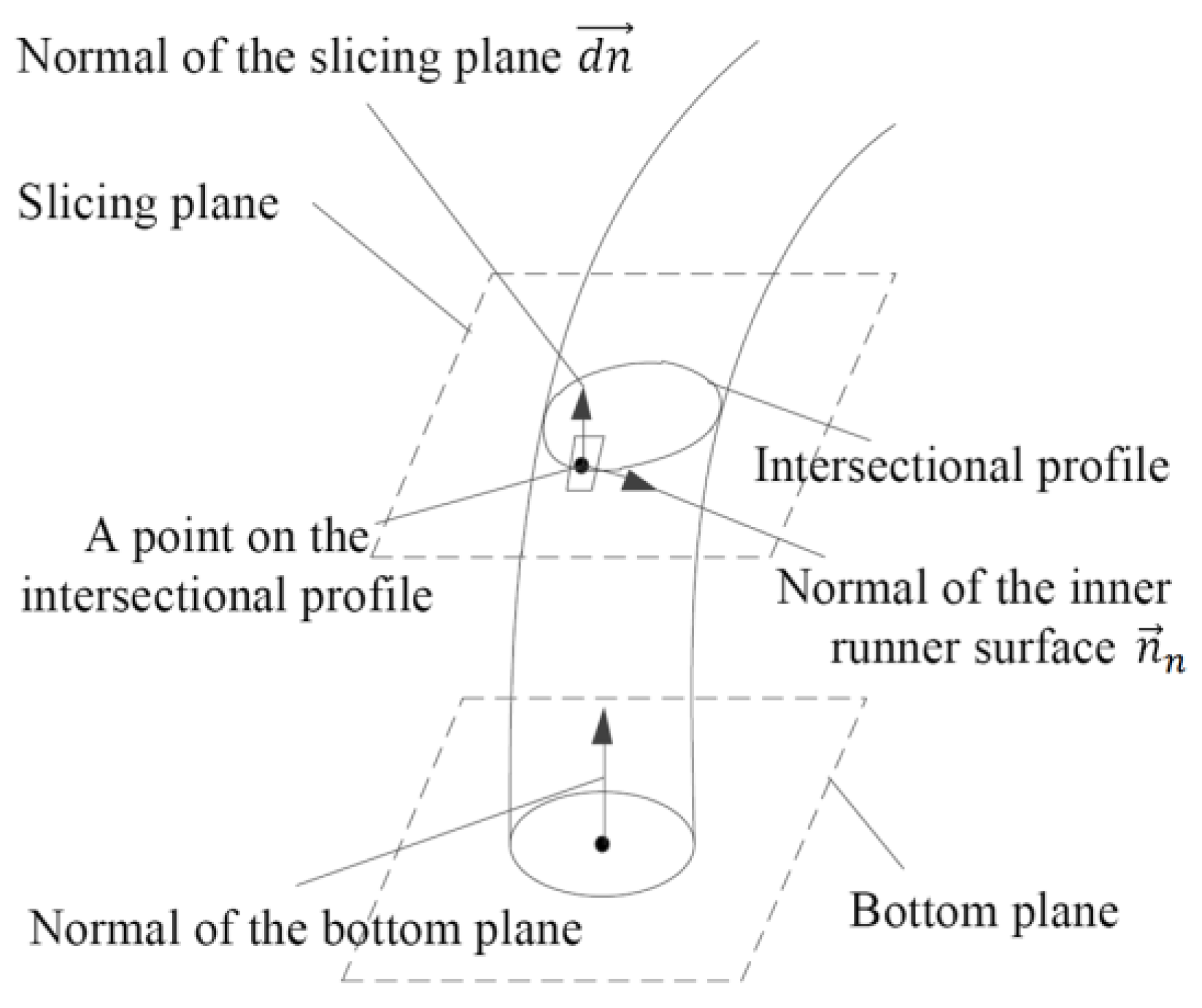
As shown in Figure 1, the initial base plane is the bottom plane, and the offset distance along the normal direction of the slicing plane is the step length. The angle between the normal directions of the inner runner surface and the slicing plane in the intersectional profile is calculated as k. When the threshold value is greater than or equal to k₀, the slicing plane stops moving.

Note that the real calculation adopts the “stl” format, in which the inner runner surface is approximated by a number of triangle facets, so the value of k needs to be calculated for the corresponding times and the largest one is selected.

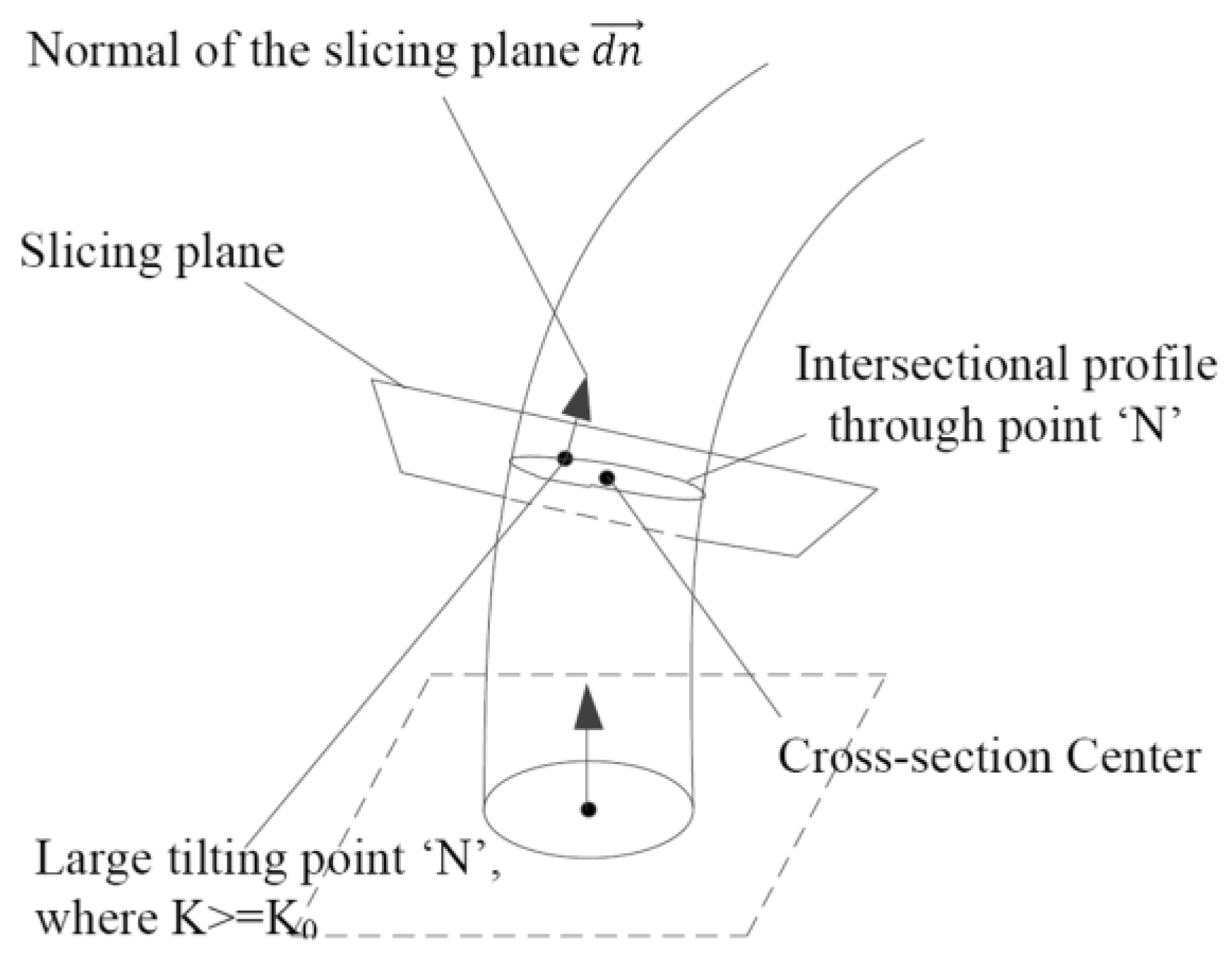
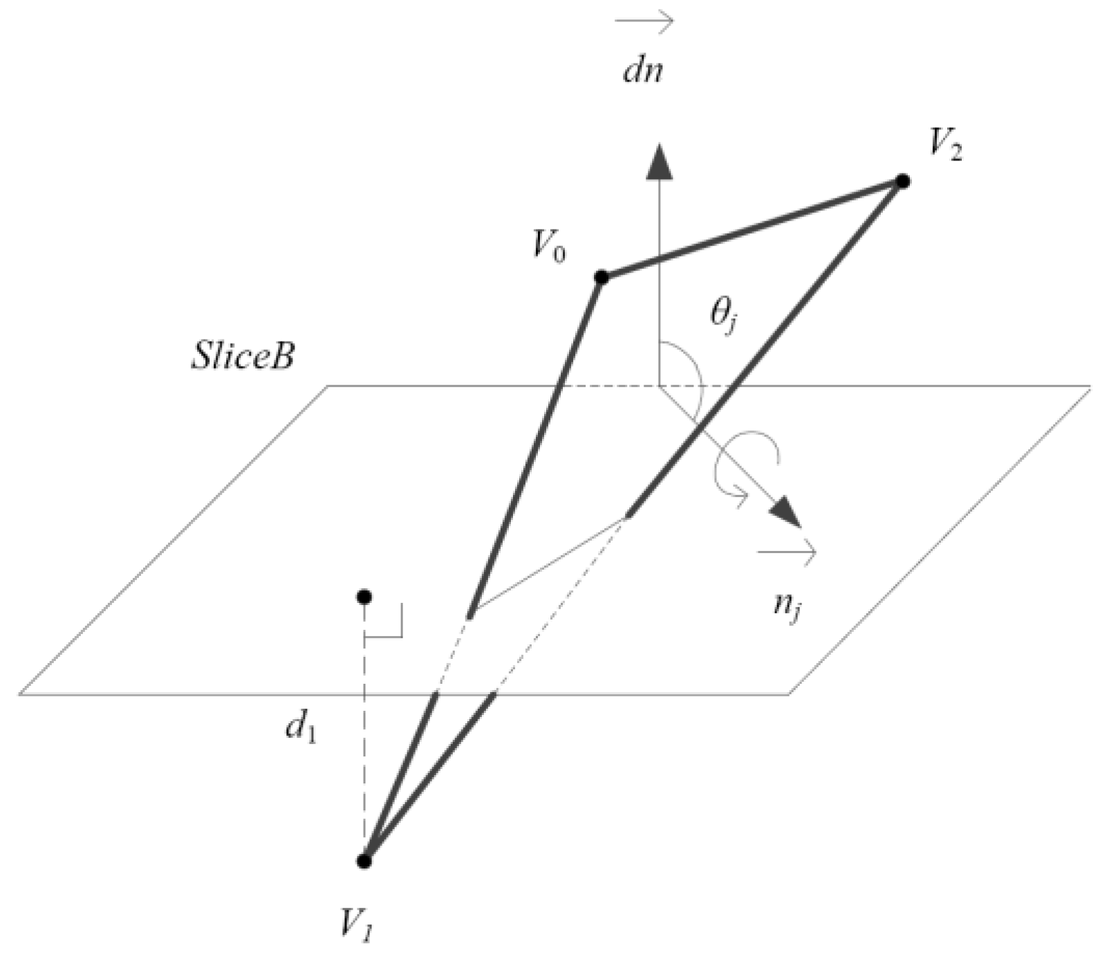
2.2. Determine a Partitioning Plane

Choose the point N where the largest k < k₀ occurs (since there are a number of facets intersecting with one slicing plane) in the last slicing plane. A new partitioning plane can be created through point N, using $\overrightarrow{dn}$ as the normal vector, as shown in Figure 2.

Choose the new partitioning plane as the new base plane, and continue the calculation as introduced above in the direction of $\overrightarrow{dn}$. Thus, all the partitioning planes can be acquired by repeating the processes in subsections A and B.

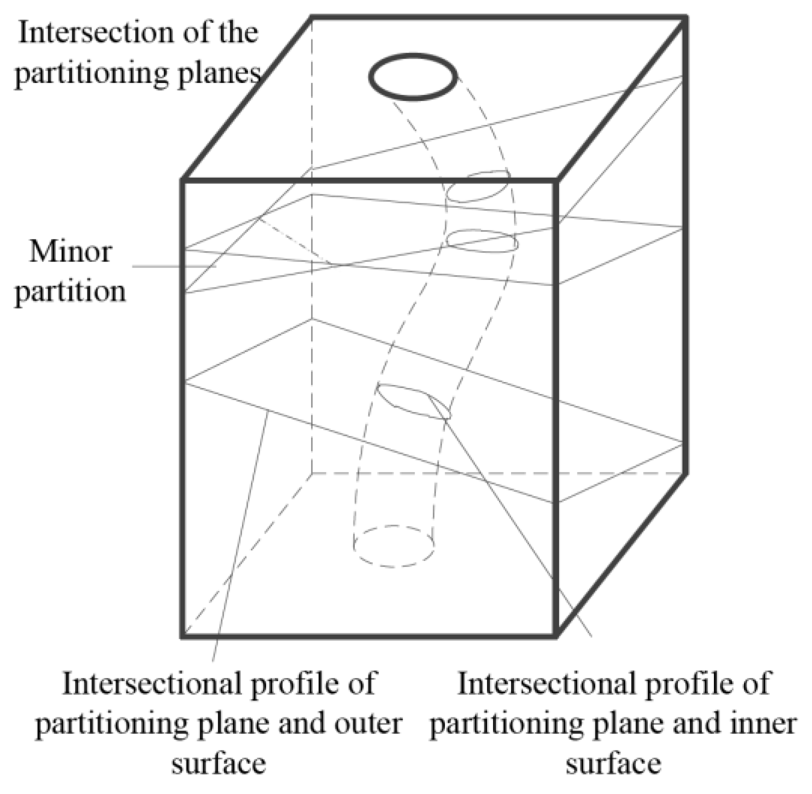
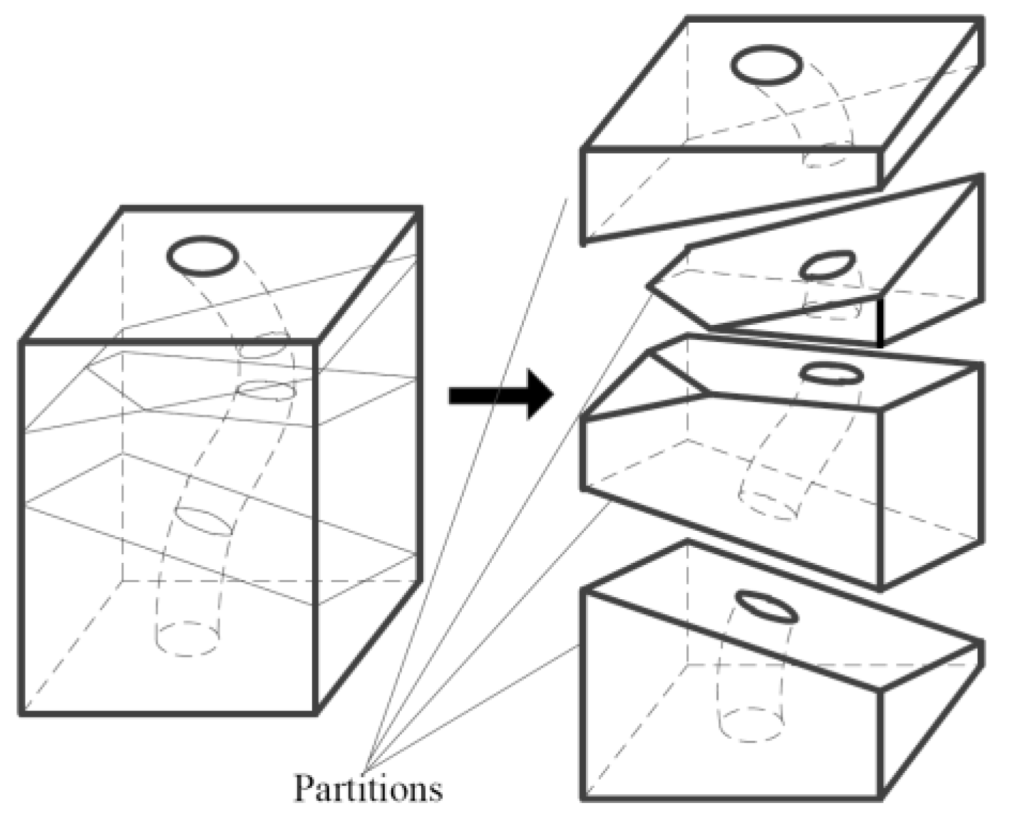
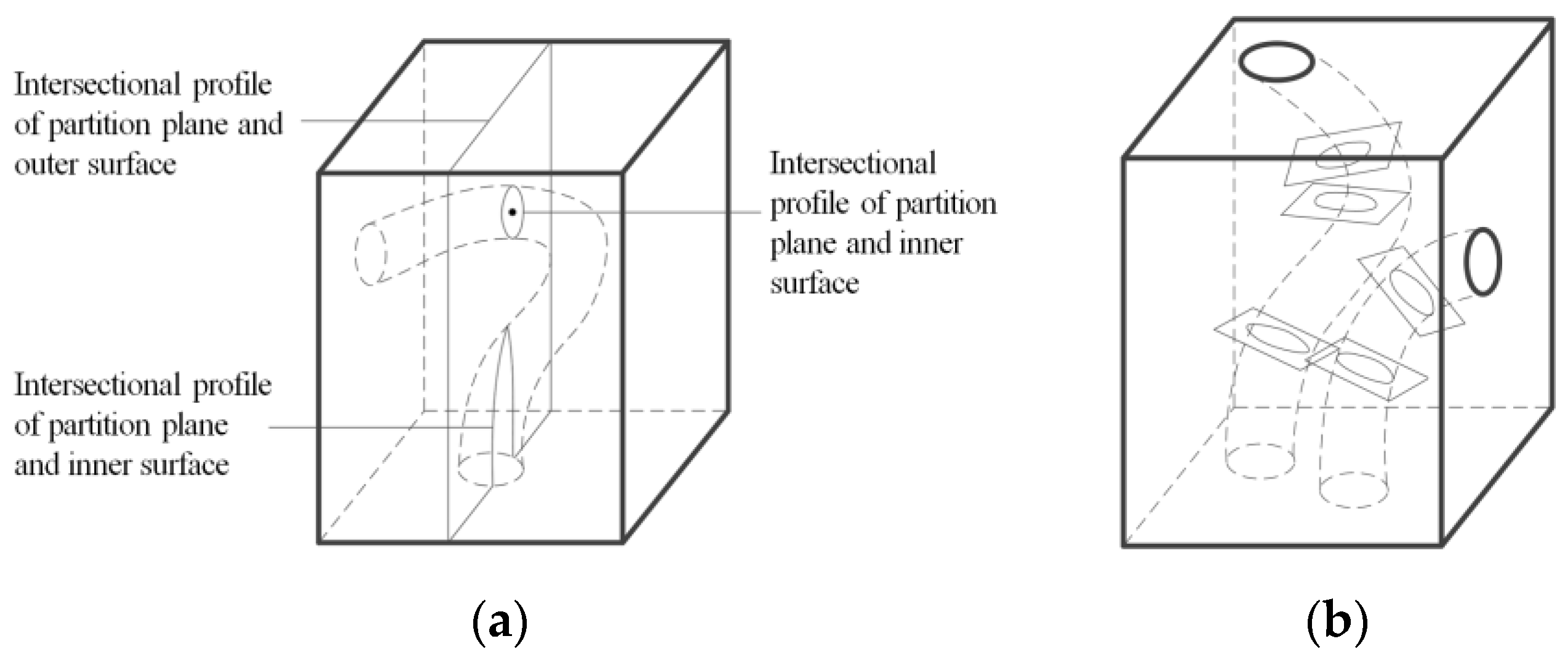
2.3. Top-to-Bottom Partitioning

Some of the partitioning planes may intersect with each other, causing minor partitions as shown in Figure 3, if the thickness between the workpart’s outer surface and the surface of the inner runner is too large. However, for thin-wall hollowed workparts, the partitioning process is completed and all the partitioning planes are determined. To avoid those minor partitions, by simplifying the following slicing processes, a “Top to Bottom” partitioning process can be used. First, the workpart is partitioned by the last calculated partitioning plane from the top, by the one before the last, and so on until the initial base plane. In this way, a workpart like that in Figure 3 can be partitioned to a series of sub-models as shown in Figure 4.

2.4. Sub-Model Partitioning for Outer Surface

All the sub-models can be support-free-printed according to the inner runner surface, when the workpart is partitioned by the process above. But some of the outer surface may now encounter the overhanging issues, because for each base plane, some surfaces may incline too much outward to hold the melt material at the right position during 3D printing. Taking the partition result of Figure 4 as an example, a discussion follows on a process to solve this emerging issue.

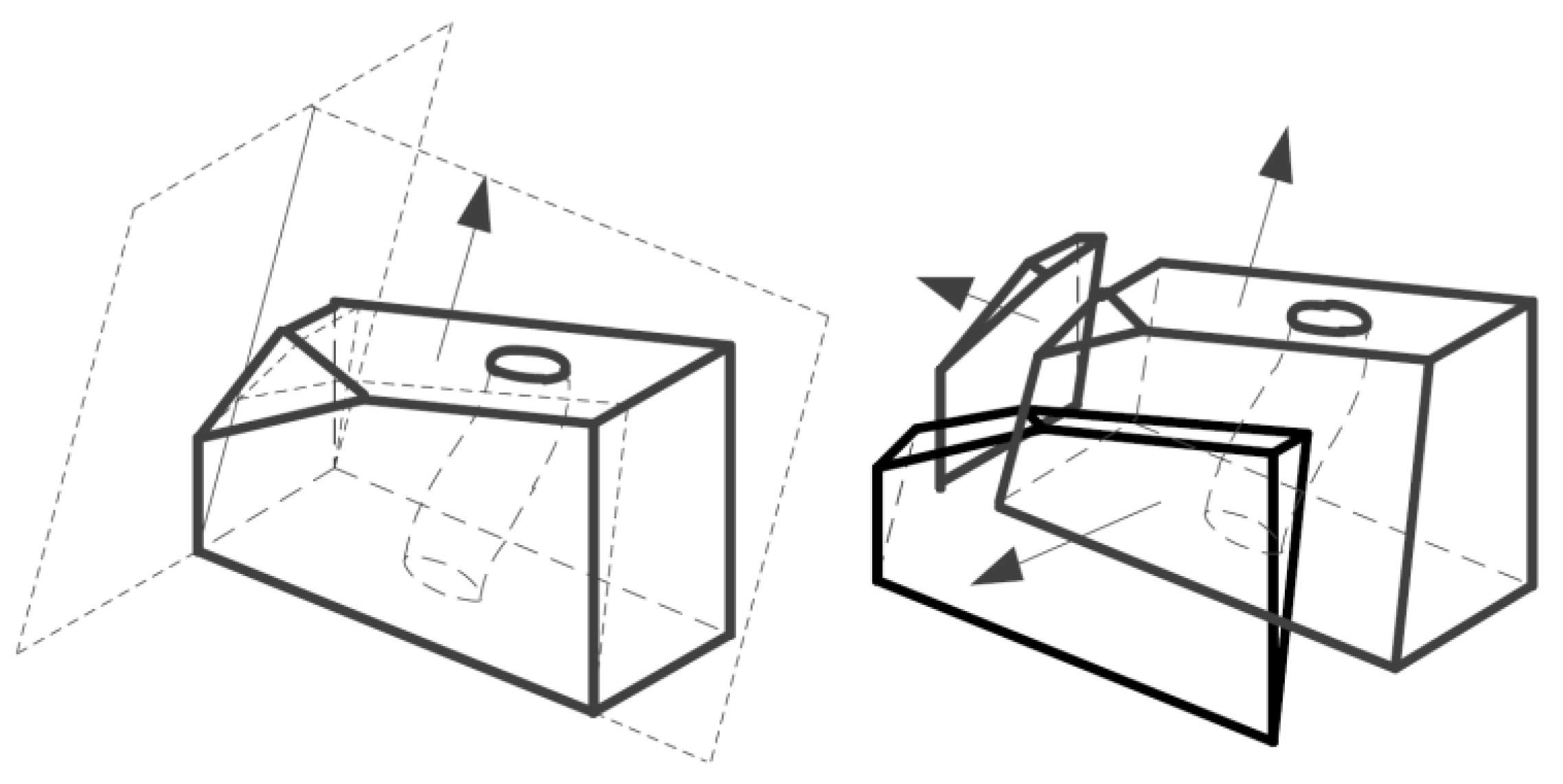
As shown in Figure 5, two planes are created perpendicular to the base plane, passing through the two corresponding edges at the bottom, and the sub-model is partitioned again into three pieces. For the largest one, the part can be sliced through the normal direction of its base plane, and for the two small ones, they can be sliced through the normal direction of the newly created partitioning planes. In the LMD processes, these three parts can be constructed using multi-axis 3D printing equipment, without any support structures. And then all those partitions can be constructed one by one without any soldering process.

In all, our plan is to partition the workpart considering the support-free slicing issue for the inner runner first, and then solve the non-support problem for the sub-models for the outer surface, using a second partitioning and slicing process. Finally, the whole part can be 3D-printed using multi-axis LMD equipment without support structures. Detailed calculation processes considering the inner runner are discussed in the following sections. Note that the methods for solving the support-free problem for the outer surface are not included in this paper, because this issue has already been solved by many researchers mentioned in the introduction.

3. Position Calculations for the Partitioning Plane

A point position and a normal vector are necessary for determining a new plane; thus, in this section, the point position calculation for the partitioning plane is explained in detail. All the calculations in this paper are based on the “stl” format.

3.1. The Pre-Slicing Method

Initially, the bottom plane is chosen as the first partitioning plane (base plane), and a value of s is set as the scanning step length, which is the distance that the slicing plane moves along its normal direction in every step. With these two parameters, a series of planes can be created for a pre-slicing process along the normal of the base plane, searching for a facet whose inclination toward the pre-slicing plane is large enough to cause a failure of the melted material deposition in the current direction.

When a pre-slicing plane intersects with the inner runner, an intersectional profile is generated in a number of facets composing the surface of the runner. These facets are marked as Equation (1), the corresponding unit normal vectors are marked as Equations (2) and (3) is a unit normal vector of the current partitioning plane.

$$F_n=(F_0,F_1,F_2,\dots ,F_n)$$

(1)

$${\overrightarrow{n}}_n\in ({\overrightarrow{n}}_0,{\overrightarrow{n}}_1,{\overrightarrow{n}}_2,\dots ,{\overrightarrow{n}}_n)$$

(2)

$$\overrightarrow{dn}({dn}_x,{dn}_y,{dn}_z)$$

(3)

Thus, the dot product between $\overrightarrow{dn}$ and ~${\overrightarrow{n}}_n^T$ can be presented as Equation (4). All dot products are cosine values because $\overrightarrow{dn}$ and ${\overrightarrow{n}}_n$ are unit vectors. In Equation (4), the minimum value is presented as Equation (5).

$${\overrightarrow{n}}_n\cdot \overrightarrow{dn}=(cos{\theta }_0,cos{\theta }_1,cos{\theta }_2,\dots cos{\theta }_n)$$

(4)

$$min\left(cos{\theta }_j\right),j\in [0,n]$$

(5)

As shown in Figure 6, if the last pre-slicing plane is marked as SliceB, and if the current is SliceT, they will be related according to Equation (6), and the minimum values of Equation (4) for both SliceB and SliceT are marked as Equations (7) and (8), respectively.

$$SliceT=SliceB+s\cdot \overrightarrow{dn}$$

(6)

$$Bmin\left(cos{\theta }_j\right)$$

(7)

$$Tmin\left(cos{\theta }_k\right)$$

(8)

Therefore, the whole searching process can be described as repeat calculations of Equation (9) until the conditions of Equation (10) are satisfied.

$$\left\{\begin{array}{c}SliceB=SliceT\\ SliceT=SliceB+s\cdot \overrightarrow{dn}\end{array}\right.$$

(9)

$$\left\{\begin{array}{c}{B}_{min}=Bmin\left(cos{\theta }_j\right)>cos{\theta }_{max}\\ T_{min}=Tmin\left(cos{\theta }_k\right)⩽cos{\theta }_{max}\end{array}\right.$$

(10)

3.2. The Base Point Selection

When Equation (10) occurs, the iteration of Equation (9) will stop. The current SliceB will be called a “Restricting Plane (RP)”, and the corresponding facet where Bmin occurs will marked as B(Fj). The position of a new partitioning plane which needs to be determined is a point below the RP, making the intersecting profile of the partitioning plane and the inner runner surface remain below the RP. So, three vertices of B(Fj) should be considered prior to the other points as the base point. Set Vn(xn; yn; zn); (n = 1; 2; 3) are the coordinates of the vertices of B(Fj) and SliceB(x; y; z) = 0 is the function of SliceB; thus, the new needed base point shall satisfy SliceB(Vn) ≤ 0, which means the vertex(vertices) of B(Fi) below the RP could be selected, as shown in Figure 7. If there is not only one vertex below the RP, the closest Vl satisfying Equation (11) will be selected as the base point. The distance calculation was performed using the traditional equation of Equation (12).

$$\left\{\begin{array}{c}d\left(V_l\right)=mind\left(V_n\right)\\ d\left(V_n\right)⩽0\\ n\in (\mathrm{1,2},3)\end{array}\right.$$

(11)

$$d=\frac{\mid A_B{x}_n+B_B{y}_n+C_B{z}_n+D_B\mid }{\sqrt{A_B^2+B_B^2+C_B^2}}$$

(12)

3.3. Verification and Adjustment of Base Point Position

Sometimes, the intersection profile of the new partitioning plane and the inner runner surface may also intersect with the RP; however, once the base point is selected, the new slicing direction can be calculated and, consequently, the partitioning plane through the base point will be created. To avoid this, the base point position needs to be moved by md along the negative normal direction of the pre-slicing plane, and the md is defined by Equation (13). In Equation (13), dt is the distance between a point in the intersection profile and the RP according to Figure 8.

$$m_d=\lambda max\left(d_t\right)$$

(13)

In Equation (13), max(dt) is the maximum distance between a point in the intersection profile and the RP, while λ is the length coefficient, which is used for controlling the moving distance of the position adjustment for the base point.

4. Normal Calculations for the Partitioning Plane

With an “stl” file, the normal direction for creating the new partitioning plane has to be calculated with the vertices’ information, and the result would likely be not very close to the direction of the inner runner; however, the normal direction of the new partitioning plane should be in the direction of the inner runner, which is not available in an “stl” format file. In this section, an iteration method is introduced in detail.

4.1. The Iteration Method

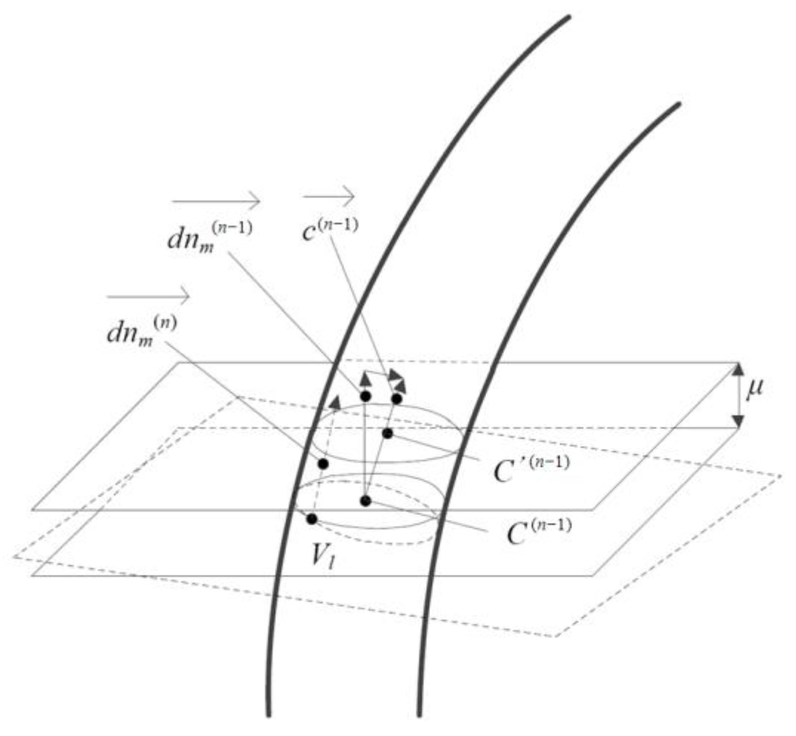
As shown in Figure 9, the normal unit vector for partitioning plane pm is defined as $\overrightarrow{d{n}_m}$, which needs to be iterated a number of times, and the iterative equation for the n-th step is defined as Equation (14), in which σ is an increment coefficient. The function $U\left(\overrightarrow{x}\right)$ is a normalizing function defined in Equation (15), and the vector $\overrightarrow{c^{(n-1)}}$ is defined in Equation (16).

$$\left\{\begin{array}{c}\overrightarrow{d{n}_m^{(n)}}=U(\overrightarrow{d{n}_m^{(n-1)}}+\sigma (\overrightarrow{c^{(n-1)}}-\overrightarrow{d{n}_m^{(n-1)}}))\\ \sigma \in (\mathrm{0,1})\end{array}\right.$$

(14)

$$U(\overrightarrow{x})=\frac{\overrightarrow{x}}{\mid \overrightarrow{x}\mid }$$

(15)

$$\overrightarrow{c^{(n-1)}}=U(C^{\mathrm{\prime }(n-1)}-C^{(n-1)})$$

(16)

In Equation (16), C⁽ⁿ⁻¹⁾ and C′⁽ⁿ⁻¹⁾ are the mass center positions of the intersection profile by the inner runner surface and the iterating partitioning planes, respectively, and the vector $\overrightarrow{c^{(n-1)}}$ is called the mass center variation vector. These three parameters are all from the iteration step n − 1, and the relative calculation processes are introduced in the following subsection B.

At the beginning of the iteration, $\overrightarrow{d{n}_m^{\left(0\right)}}$ is set as $\overrightarrow{{dn}_{m-1}}$, which is the normal unit vector of the last determined partitioning plane p_m−1. With the point V_l and the normal vector $\overrightarrow{d{n}_m^{\left(0\right)}}$, the first iterating partitioning plane $p_m^{\left(0\right)}$ can be created. The $p_m^{\left(0\right)}$ intersects with the inner runner surface, generating an intersection profile, whose mass center is C⁽⁰⁾. Then, moving plane $p_m^{\left(0\right)}$ along the $\overrightarrow{d{n}_m^{\left(0\right)}}$ for a tiny offset of μ, a new intersection profile will be generated and the corresponding mass center is C′⁽⁰⁾.

The stop condition for the iteration is defined as Equation (17), in which Φ is an angle function calculating the cosine value of the intersection angle between two assigned vectors. Φ can be defined as Equation (18).

$${\varphi }_n=\overrightarrow{d{n}_m^{\left(n\right)}}\cdot \overrightarrow{c^{\left(n\right)}}⩾{\varphi }_s$$

(17)

$$\varphi =\overrightarrow{v_a}\cdot \overrightarrow{v_b}=\mathrm{c}\mathrm{o}\mathrm{s}{\gamma }_{ab}$$

(18)

Obviously, according to Equation (18), Φ ∈ [−1, 1]. Φ_s is the iteration stop condition value, which is a constant and assigned manually. Considering with the iteration target, Φ_s should be close to 1, which means the vectors $\overrightarrow{d{n}_m^{\left(n\right)}}$ and $\overrightarrow{c^{\left(n\right)}}$ should be in very close directions.

If the stop condition is achieved at the n-th step during the iteration, the normal direction of the partitioning plane p_m will be set as Equation (19).

$$\overrightarrow{d{n}_m}=\overrightarrow{d{n}_m^{\left(n\right)}}$$

(19)

4.2. Calculations for Intersectional Profile Mass Centers

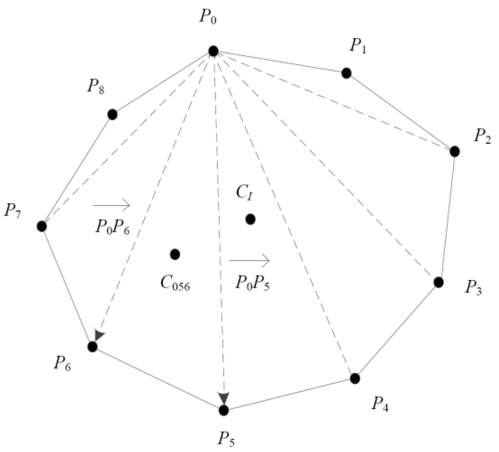
In an “stl” file, all surfaces are approximated by finite triangle facets, so the intersectional profiles are also composed by segments in the intersecting plane, as shown in Figure 10; an intersection profile has finite vertices such as (P₀, P₁, P₂,…, P_m). Then, the mass center C_I of the profile P₀P₁P₂P₃P₄P₅P₆P₇P₈ can be acquired through two steps: (1) calculate the mass centers C_0i(i+1) of all the triangles in Figure 10; (2) perform weighted calculations for all C_0i(i+1) values by each corresponding triangle size. The calculation steps can be presented as Equation (20).

$$\left\{\begin{array}{c}{A}_{0i(i+1)}=\frac{1}{2}(\overrightarrow{P_0{P}_i}\times \overrightarrow{P_0{P}_{i+1}})\cdot \overrightarrow{n_I}\\ C_{0i(i+1)}=\frac{P_0+P_i+P_{i+1}}{3}\\ C_I={\sum }_{i=1}^{m-1}{C}_{0i(i+1)}{A}_{0i(i+1)}/{\sum }_{i=1}^{m-1}{A}_{0i(i+1)}\end{array}\right.$$

(20)

where A_0i(i+1) and C_0i(i+1) are the size and the mass center of ΔP₀P_iP_i+1, respectively, and $\overrightarrow{n_I}$ and C_I are the normal unit vector and the mass center of the intersection profile P₀P₁P₂P₃P₄P₅P₆P₇P₈, respectively.

4.3. Discussions of the Convergence

In order to acquire an ideal result from Equation (14), the iteration has to be convergent to satisfy the condition defined in Equation (21), in which $\overrightarrow{v}$ is the direction of the inner runner and theoretically shall be the tangent unit vector of the guideline; however, it is approximated by $\overrightarrow{c^{\left(n\right)}}$. Thus, Equation (21) means the result in the n step has to always be closer to $\overrightarrow{v}$ than that in the n − 1 step until Equation (17) is satisfied.

$$\overrightarrow{d{n}_m^{\left(n\right)}}\cdot \overrightarrow{v}>\overrightarrow{d{n}_m^{(n-1)}}\cdot \overrightarrow{v}$$

(21)

Equation (21) can also be rewritten in the form of Equation (22), which means that, every time, the vector $\overrightarrow{d{n}_m^{\left(n\right)}}$ should not go too far toward the vector $\overrightarrow{v}$ in each step of the iteration, so the value of σ should not be too large.

$$(\overrightarrow{d{n}_m^{\left(n\right)}}-\overrightarrow{d{n}_m^{(n-1)}})\cdot \overrightarrow{v}>0$$

(22)

Also, according to Equation (14), set M is the modulus of $\overrightarrow{d{n}_m^{\left(n\right)}}+\sigma (\overrightarrow{c^{\left(n\right)}}-\overrightarrow{d{n}_m^{\left(n\right)}})$, and the relationship between M and σ can be derived as Equation (23), in which γ is the angle between $\overrightarrow{d{n}_m^{\left(n\right)}}$ and $\overrightarrow{c^{\left(n\right)}}$. It is obvious that when Φ ∈ [0, π/2], M is a monotonic function for γ; thus, only if the value of σ is small enough, the iteration can stop upon satisfying the condition of Equation (17), and at this time, M should be a value which is smaller than but very close to 1.

$$M^2={\sigma }^2+(1-\sigma {)}^2+2\sigma (1-\sigma )\mathrm{c}\mathrm{o}\mathrm{s}\gamma$$

(23)

4.4. Analysis of Applicable Conditions

The partitioning method is not applicable to all parts with an inner runner. The applicability analysis is conducted below to clarify the limitations of this method’s application.

(1)

The partitioning plane cannot intersect with the bottom surface. If, for some reason, such as a large change in the direction of the inner runner, only a portion of the bottom surface can be printed at the beginning, then the subsequent printing process will be difficult to achieve, as shown in Figure 11a.

(2)

Only one inner runner contour can be present in the model to obtain a determined partitioning plane. As shown in Figure 11b, there are two inner runners in the model and the directions of each runner are different. Two sets of different partitioning planes will be generated, causing the model to be unable to correctly partition. To address this situation, it is necessary to pre-partition the model before implementing this method.

5. Algorithm Analyses

A set of programs were developed in Python 3.7.3 (Python Software Foundation, Wilmington, DE, USA) and the VTK 8.1.2 visualization toolkit (Kitware Inc., Clifton Park, NY, USA). A series of tests were carried out for assessing and adjusting the algorithm with some variables, and the result is discussed in detail in this section. All the physical meanings of the variables are listed below.

• α—the angle between the normal of a facet and the fabrication direction.
• γ—the angle between $\overrightarrow{d{n}_m^{\left(n\right)}}$ and $\overrightarrow{c^{\left(n\right)}}$.
• θ—tilt angle, α = θ + π/2.
• il—tilt limit, il = cosα_max.
• s—scanning step length, the distance for the slicing plane to move along its normal direction in every step in pre-slicing process.
• μ—offset, the tiny distance in Figure 9, used for calculating Equation (16).
• Φ—proximity, Φ = cosγ.
• Φ_s—proximity requirement, set manually, for stopping the iteration.
• σ—increment coefficient in Equation (14).
• $\lambda$—length coefficient in Equation (13).
• f_c—cosine value of the angle between the normal of the inner runner facet at the current partitioning plane P_m and the normal of the former partitioning plane P_m−1.
• m_c—the minimum cosine value of the angles between the normals of the inner runner facets at P_m and the normal of P_m.

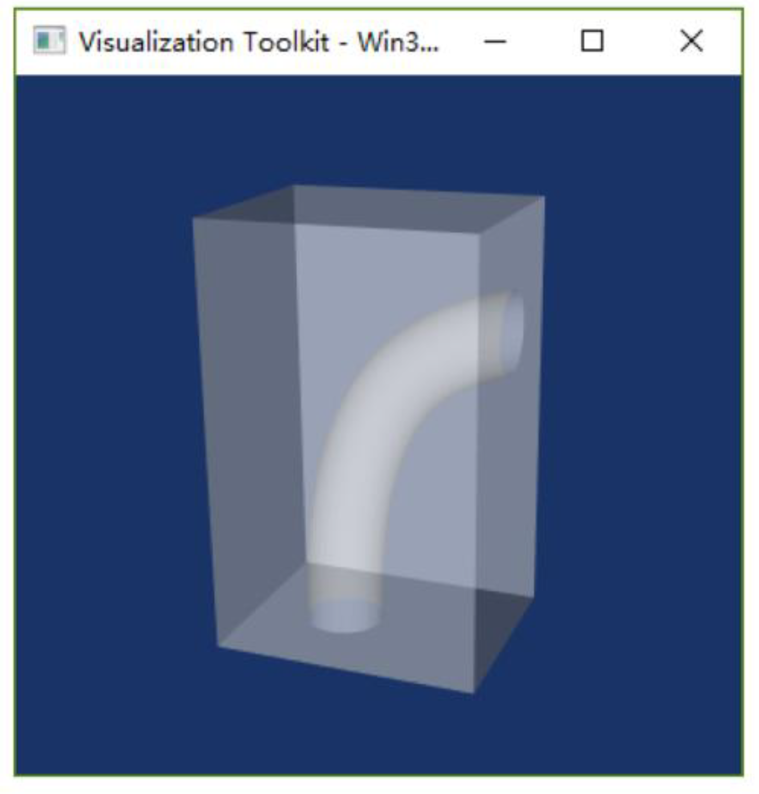
The analysis is carried out by investigating the influence of the variation in Φ_s and σ on the partitioning result and the calculation process with a test “stl” model. As shown in Figure 12, the test model is a 50 mm × 40 mm × 80 mm cuboid with a single-direction crooked inner runner.

5.1. Influences from Φ_s to the Partitioning Results

Φ defines the proximity of two vectors, and it is a cosine value of the angle between the partitioning plane’s normal direction and the mass center vector, $\overrightarrow{c}$. The closer Φ is to 1.0, the more likely that the two vectors will have the same direction. Φ_s is set manually as a requirement of proximity from the partitioning plane’s normal vector to the mass center variation vector $\overrightarrow{c}$. Φ_s has a significant influence on the calculation process, because the iteration stops only if Φ ≥ Φ_s is satisfied. 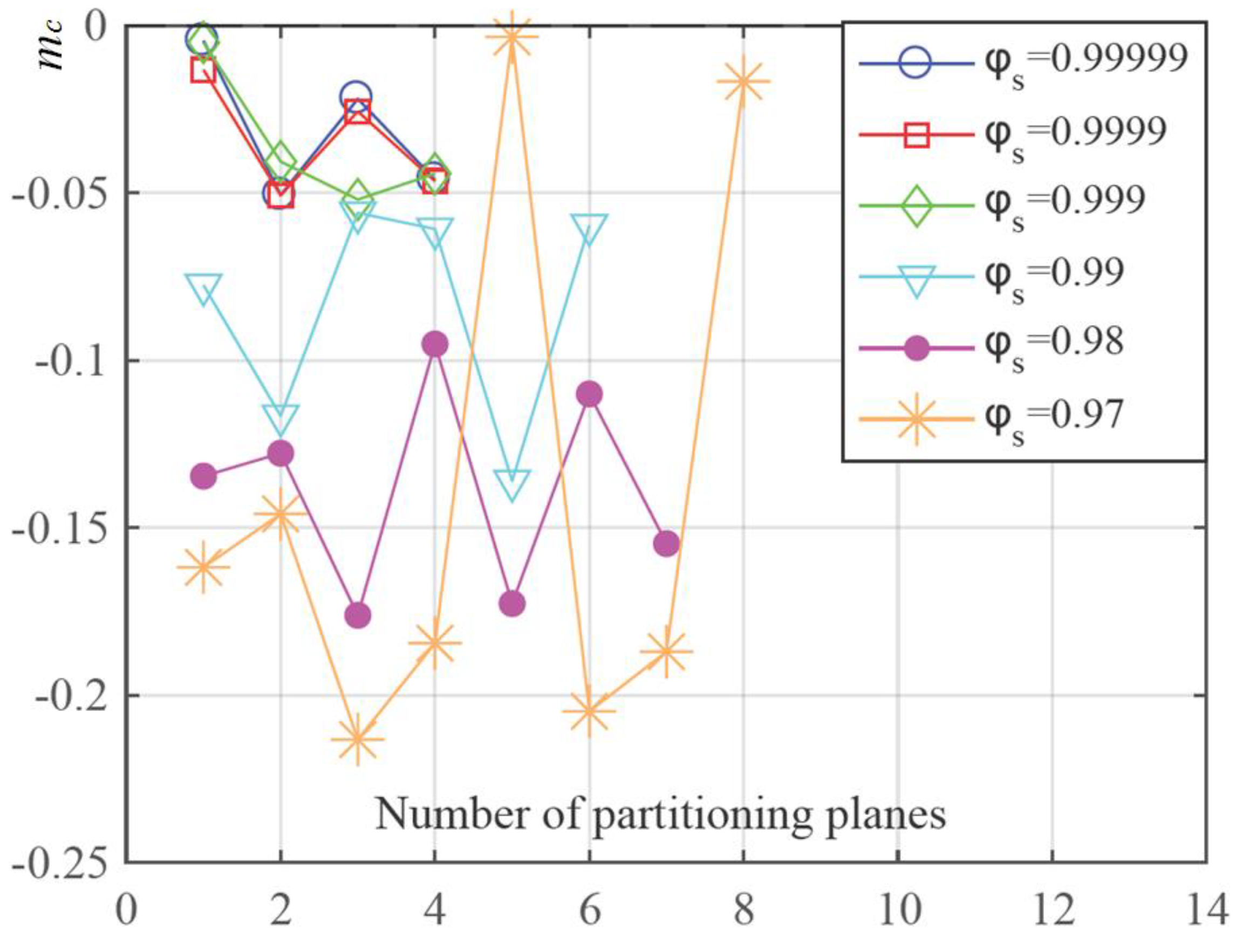So, the following analysis was carried out by varying Φ_s with il set to –0.2924, the scanning step length s set to 0.7, the offset μ set to 0.01, and the increment coefficient σ set to 1/8. The result is listed in

Table 1. Test results by Φ_s.

$\mathit{i}\mathit{l}=-0.2924\hspace{1em}\mathit{s}=0.7\hspace{1em}\mathit{\mu }=0.01\hspace{1em}\mathit{\sigma }=1/8\hspace{1em}\mathit{\lambda }=1.5$
φs	No. PP	mc	fc
0.97	1	−0.161757	−0.257633
	2	−0.145814	−0.281714
	3	−0.213203	−0.287227
	4	−0.184432	−0.291998
	5	−0.003358	−0.249331
	6	−0.204769	−0.275151
	7	−0.186980	−0.245675
	8	−0.016641	−0.239250
0.98	1	−0.134533	−0.257633
	2	−0.127699	−0.257868
	3	−0.176095	−0.275733
	4	−0.095078	−0.255620
	5	−0.172584	−0.270708
	6	−0.109987	−0.260786
	7	−0.154680	−0.279234
0.99	1	−0.077480	−0.257633
	2	−0.116569	−0.291271
	3	−0.055903	−0.254650
	4	−0.060716	−0.239921
	5	−0.136024	−0.257967
	6	−0.059599	−0.239716
0.999	1	−0.005015	−0.257633
	2	−0.040578	−0.269465
	3	−0.051910	−0.235418
	4	−0.044187	−0.291792
0.9999	1	−0.013161	−0.257633
	2	−0.050654	−0.261617
	3	−0.025590	−0.224373
	4	−0.046411	−0.266750
0.99999	1	−0.004503	−0.257633
	2	−0.050597	−0.269991
	3	−0.021840	−0.224427
	4	−0.046025	−0.263151

No. PP: number of partitioning planes.

, and Figure 13 presents the relationships between mc, Φ_s, and the final number of partitioning planes generated.

According to Figure 13, when Φ_s was set to smaller values, more partitioning planes were finally acquired, and during the whole process, smaller mc values were achieved. In contrast, if Φ_s was set to values closer to 1.0, fewer partitioning planes could be generated and greater mc values closer to 0.0 could be achieved.

Theoretically, a smaller mc value indicates a large angle between the normal directions of the facet and the partitioning plane where they interact with each other. This also revealed that a large angle was present between the guideline of the inner runner and the normal direction of the partitioning plane. Under this condition, the partitioning plane did not perform well, a large tilting angle was still present between the inner runner and the partitioning plane, and even the construction direction changed along the normal of the generated partitioning plane. Consequently, the following would repeatedly take place as the scanning continued: il would be reached sooner, the new partitioning plane would be generated with a small Φ_s, and finally a greater number of partitioning planes would be achieved.

From this point of view, a greater value for Φ_s will help to reduce the number of partitioning planes, and for each plane, the angle between the normal directions of the facet of the inner runner and the partitioning planes will also be decreased. However, there will not always be a better result for a larger value of Φ_s. Also, as shown in Table 1 and Figure 13, the value of mc had no significant changes when Φ_s was set to 0.999, 0.9999, and 0.9999, meaning that Φ_s = 0.999 was large enough compared with the other two values. Thus, in this point of view, a proper Φ_s shall be selected, or if an even greater value is set, more calculation time and resources will be spent.

It is important to point out that Φ_s = 1.0 is an ideal situation which will never be adopted, for following three reasons:

(1)

It is meaningless. As we know from Equation (14), the aim of the iteration is to turn the $\overrightarrow{d\mathrm{n}}$ vector into a direction close to $\overrightarrow{c}$, which is actually used for approximating the guiding line direction. At this point, a Φ_s = 1.0 requirement is to make the $\overrightarrow{d\mathrm{n}}$ vector turn toward the same direction as $\overrightarrow{c}$ (but not the real guiding line direction), which does not make sense.

(2)

Errors have already existed, as the program worked on the “stl” files which use triangle facets to approximate all the workparts’ surface features. Thus, Φs = 1.0 would theoretically not achieve a better result than a smaller value.

(3)

It took too much calculation time, because on the one hand, to turn the vector into a more accurate angle but not a range, the increment coefficient σ has to be set to a very small value. In this way, many more iteration steps will be required. On the other hand, from Figure 13, when Φ_s is great enough, better results will not be achieved with an even larger value, but more calculation resources will be consumed.

Besides the above, from the fourth column of Table 1, it was clear that during all the calculations, every f_c value was smaller than the set il, indicating that our method succeeded in partitioning the model for the support-free LMD process.

5.2. Influences from σ to the Partitioning Results

The increment coefficient σ is used for controlling the iteration increments, which is defined by the product of σ, the differential vector of the partitioning plane’s normal unit vector $\overrightarrow{dn}$, and the mass center variation vector $\overrightarrow{c}$, according to the iteration equation (Equation (14)).

Table 2. Test results for σ.

$\mathit{i}\mathit{l}=-0.2924\hspace{1em}\mathit{s}=0.7\hspace{1em}\mathit{\mu }=0.01\hspace{1em}{\mathit{\Phi }}_{\mathit{s}}=0.9999\hspace{1em}\mathit{\lambda }=1.5$
$\mathit{\sigma }$	No. PP	mc	fc	I.T.
1/2	1	−0.009083	−0.257633	14
	2	-	-	-
1/4	1	−0.011499	−0.257633	18
	2	-	-	-
1/8	1	−0.013161	−0.257633	37
	2	−0.050654	−0.261617	19
	3	−0.025590	−0.224373	19
	4	−0.046411	−0.266750	13
1/16	1	−0.014245	−0.257633	72
	2	−0.051053	−0.203020	33
	3	−0.026169	−0.223983	39
	4	−0.046481	−0.267314	27
1/32	1	−0.014045	−0.257633	145
	2	−0.050863	−0.203216	67
	3	−0.026438	−0.224168	79
	4	−0.046514	−0.267576	55

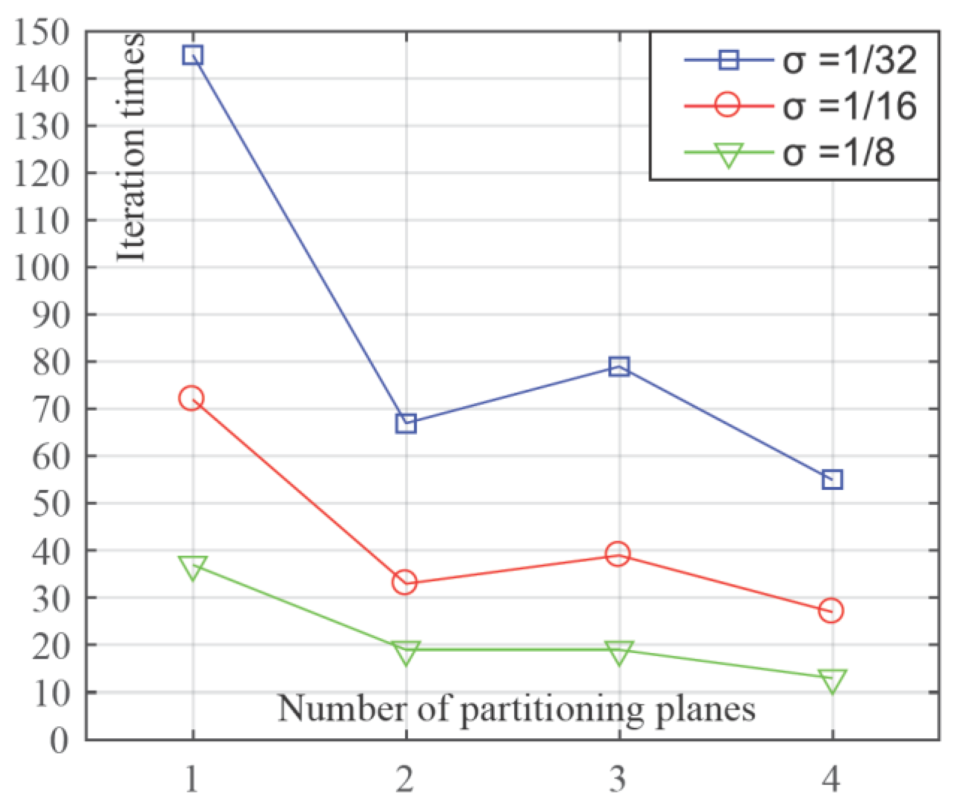
No. PP: number of partitioning planes. I.T.: iteration times.

and Figure 14 show the test results of the influence from a varying increment coefficient, with related parameters set as il = −0.2924, s = 0.7, μ= 0.01, Φ_s = 0.9999, and λ = 1.5. From Table 2, when σ was set to greater values of 1/2 or 1/4, only the first partitioning plane was fully acquired, but for the second plane, the iteration did not converge to the desired range of Φ_n ≥ Φ_s. This means that the program knows that a partitioning plane is needed here, but the normal direction of the plane cannot be acquired. As a comparison, when σ was set to smaller values such as 1/8, 1/16, and 1/32, all four partitioning planes were fully acquired. From the third column of Table 2, as σ became smaller, the m_c values did not change much, because all iterations stopped when Φ_n ≥ Φ_s was satisfied. From this point of view, for the same given value of Φ_s, the iteration result will almost be the same for the variation in σ.

On the other hand, from Figure 14, the value of σ influenced the total number of iteration steps for acquiring the same partitioning plane. It is clear that when σ was reduced to half its value, the total number of iteration steps would be doubled for calculating the same plane, causing more calculation time to be spent.

In all, for a certain Φ_s, too great a σ value will cause the convergence of the iteration to fail; when the convergence is valid, the iteration result will be almost the same for different σ values; a smaller σ will cause more iteration steps.

Also, from the fourth column of Table 2, the f_c value was always greater that il, indicating that the algorithm worked successfully for support-free partitioning.

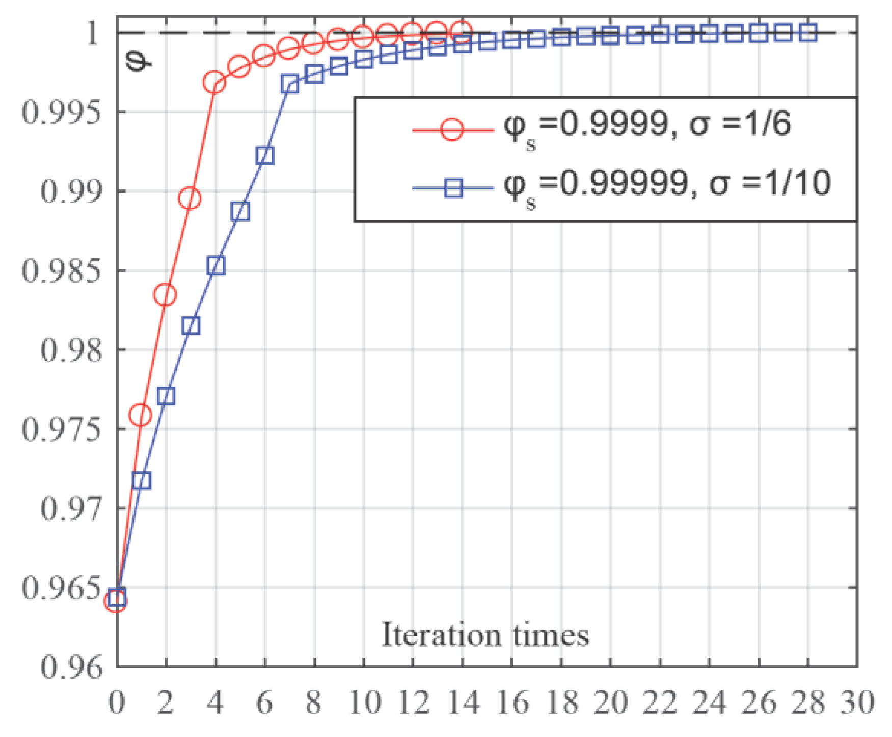
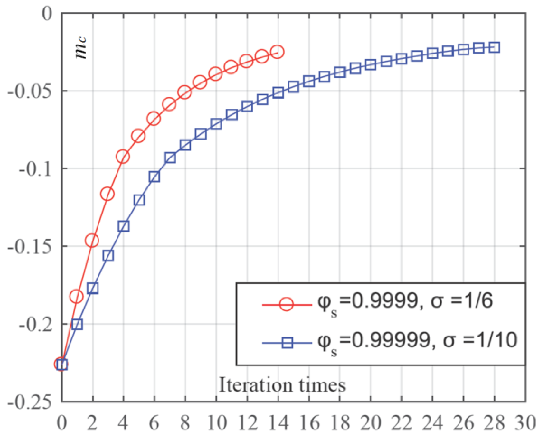
5.3. Analysis of the Iteration Process

Two calculation processes for iterating the third partitioning plane are presented here for comparison. In one process, Φ_s was set to 0.9999 and σ was set to 1/6, while in the other process, Φ_s was set to 0.99999 and σ was set to 1/10. The other parameters were set to the same values in the two processes as il = −0.2924, s = 0.7, and μ = 0.01.

Table 3. Data from iteration test 1.

$\mathit{i}\mathit{l}=-0.2924\hspace{1em}\mathit{s}=0.7\hspace{1em}\mathit{\mu }=0.01\hspace{1em}{\mathit{\Phi }}_{\mathit{s}}=0.9999\hspace{1em}\mathit{\sigma }=1/6\hspace{1em}\mathit{\lambda }=1.5$
I. Step	${\mathit{\varphi }}_{\mathit{n}}$	mc	fc
0	0.964026	−0.226507	−0.226507
1	0.975772	−0.182994	−0.226507
2	0.983359	−0.146965	−0.226507
3	0.989437	−0.116933	−0.226507
4	0.996767	−0.092912	−0.226507
5	0.997755	−0.079589	−0.226507
6	0.998441	−0.068473	−0.226507
7	0.998917	−0.059203	−0.226507
8	0.999248	−0.051474	−0.226507
9	0.999478	−0.045031	−0.226507
10	0.999638	−0.039661	−0.226507
11	0.999748	−0.035186	−0.226507
12	0.999825	−0.031456	−0.226507
13	0.999879	−0.028348	−0.226507
14	0.999916	−0.025503	−0.224562

I. step: iteration step.

and

Table 4. Data from iteration test 2.

$\mathit{i}\mathit{l}=-0.2924\hspace{1em}\mathit{s}=0.7\hspace{1em}\mathit{\mu }=0.01\hspace{1em}{\mathit{\Phi }}_{\mathit{s}}=0.99999\hspace{1em}\mathit{\sigma }=1/10\hspace{1em}\mathit{\lambda }=1.5$
I. Step	${\mathit{\varphi }}_{\mathit{n}}$	mc	fc
0	0.964364	−0.226288	−0.226288
1	0.971713	−0.200400	−0.226288
2	0.977065	−0.177190	−0.226288
3	0.981492	−0.156186	−0.226288
4	0.985288	−0.137244	−0.226288
5	0.988720	−0.120303	−0.226288
6	0.992218	−0.105431	−0.226288
7	0.996756	−0.093054	−0.226288
8	0.997372	−0.085049	−0.226288
9	0.997871	−0.077839	−0.226288
10	0.998276	−0.071346	−0.226288
11	0.998603	−0.065499	−0.226288
12	0.998869	−0.060234	−0.226288
13	0.999084	−0.055495	−0.226288
14	0.999258	−0.051228	−0.226288
15	0.999399	−0.047387	−0.226288
16	0.999513	−0.043930	−0.226288
17	0.999606	−0.040818	−0.226288
18	0.999681	−0.038017	−0.226288
19	0.999741	−0.035497	−0.226288
20	0.999791	−0.033228	−0.226288
21	0.999830	−0.031186	−0.226288
22	0.999863	−0.029348	−0.226288
23	0.999889	−0.027694	−0.226288
24	0.999910	−0.025944	−0.224319
25	0.999928	−0.024617	−0.224319
26	0.999957	−0.023432	−0.224319
27	0.999982	−0.022511	−0.224319
28	0.999991	−0.021917	−0.224319

I. step: iteration step.

show the data generated in relative iterations. With these data, Figure 15 and Figure 16 were created to reveal the relationships between Φ and the number of iteration steps as well as m_c and the number of iteration steps in the same calculation work with different pre-set parameters.

As shown in Figure 15, the value of Φ increased sharply at about the first 1/4 of the total iteration steps, and then this acceleration decreased to quite a small value, increasing the Φ value little by little until the desired value of Φ_s was exceeded. Also, Figure 16 indicates that the increasing speed of the mc value would slow down with the increase in the iteration steps, and, finally, m_c would converge.

During the iteration, the mass center variation vector of the intersectional profile of the inner runner and the pre-partitioning planes was not a constant, because in each iteration step, new pre-partitioning planes would be created with an adjusted direction; however, the iteration calculations still turn the normal of the pre-partitioning plane into a direction that was very close to the mass center variation vector. Thus, from the situation presented by Table 3 and Table 4 and Figure 15 and Figure 16, it was believable that the iteration algorithm in this paper was convergent, and in all, through the calculation, the f_c values were greater than the required il values, which also backed up the algorithm’s convergence.

6. An Application Test

The runner profile used in the section above is too simple to fully verify the capability of the support-free algorithm. So, in this section, a model with more complicated features is used for extensive testing, and the results are listed for the assessment to see whether the algorithm was still capable of solving the support-free partitioning problem. A simple outer profile is used here because the method in this paper focuses on solving support-free-printing inner runner problems, and the methods for the outer profiles are already developed.

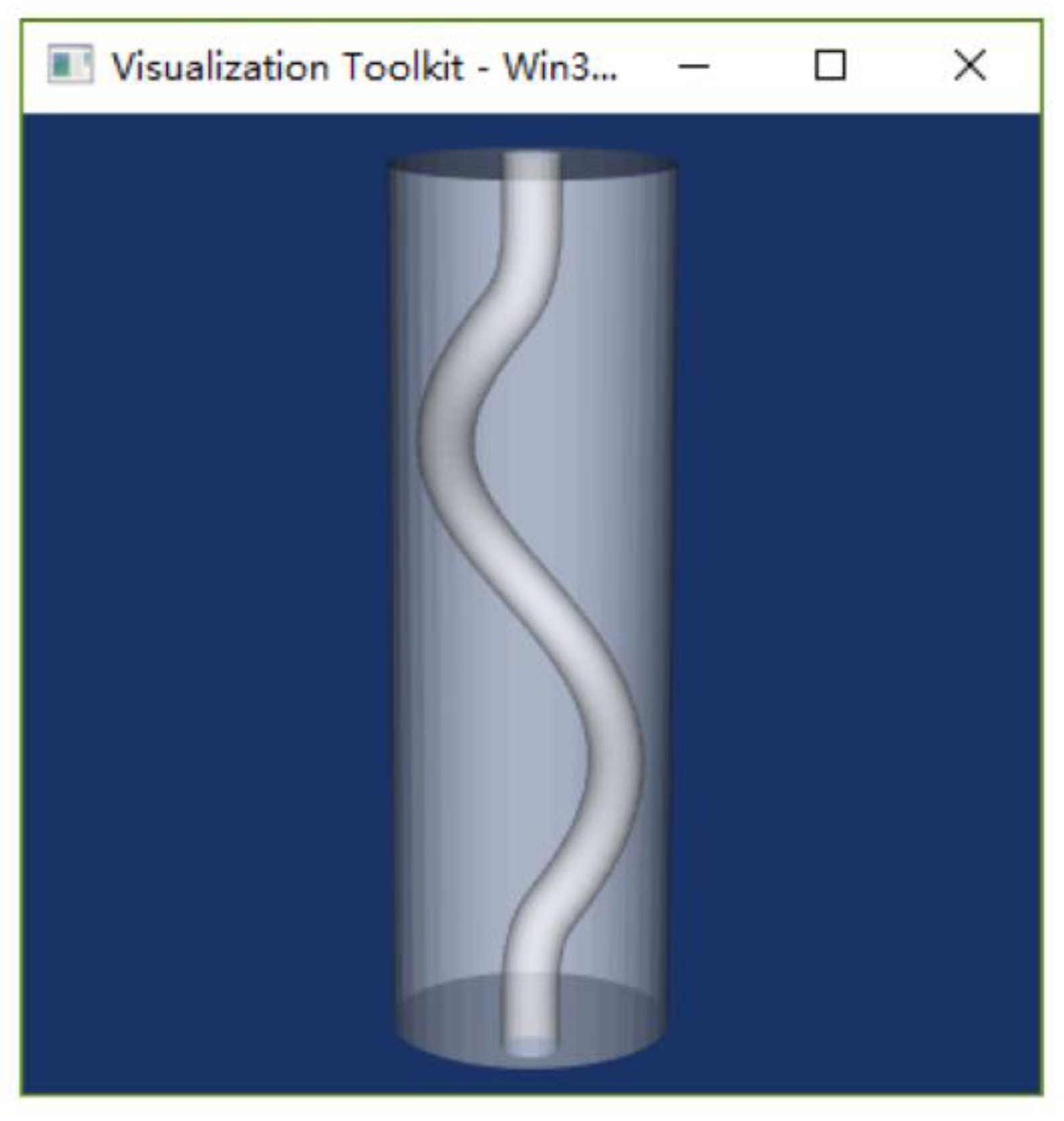
As shown in Figure 17, the model was a Φ50 mm × 150.83 mm column outside with a compound inner runner inside, which was composed of two parts of straight runners at both ends, a three-dimensional spiral runner in the middle, and smooth transitions among the three parts. The diameter of the spiral runner was Φ10 mm, the diameter of the spiral was Φ30 mm, the rotation angle was 330°, and the pitch was 110 mm; the diameter of the inner straight runner was also Φ10 mm and the length was 10 mm.

The solution process was performed with the following parameters: the tilting limit il = −0.34, of which the corresponding intersecting angle (between the facet and the fabricating direction) was 19.88°; scanning step length s = 0.7; offset μ = 0.01; proximity Φ_s = 0.9999; and increment coefficient σ= 1/16. The algorithm was run on a regular computer with an i3 processor and 8 GB of memory, with a solution time of 8 s. The solution output data are listed in

Table 5. Data output from the application test.

$\mathit{i}\mathit{l}=-0.34\hspace{1em}{\mathit{\theta }}_{\mathbf{m}\mathbf{a}\mathbf{x}}=19.88^{\circ }\hspace{1em}\mathit{s}=0.7$ $\mathit{\mu }=0.01\hspace{1em}{\mathit{\Phi }}_{\mathit{s}}=0.9999\hspace{1em}\mathit{\sigma }=1/16\hspace{1em}\mathit{\lambda }=1.5$
PP	mc	fc	No. IS
1	−0.044808	−0.248650	47
2	−0.058916	−0.291692	30
3	−0.047030	−0.293546	44
4	−0.014190	−0.306148	56
5	−0.043214	−0.324324	43
6	−0.033065	−0.322172	57
7	−0.013896	−0.319341	57
8	−0.043283	−0.324528	43
9	−0.033151	−0.322213	57
10	−0.013828	−0.319260	57
11	−0.043234	−0.324650	43
12	−0.033131	−0.322206	57
13	−0.013707	−0.319218	58
14	−0.055656	−0.329826	45
15	−0.066840	−0.265796	36

PP: partitioning plane. No. IS: number of iteration steps.

, illustrating that 15 partitioning planes were finally acquired, and the maximum number of iteration steps for calculating each plane was 58, the minimum m_c value was −0.066840 with the corresponding intersecting angle of 3.83°, and for the spiral runner part, the minimum m_c value was −0.047030 with the corresponding intersecting angle of 2.7°. These two intersecting angles were both far less than the tilting limit of 19.88°, indicating that the change in the contribution direction by the partitioning planes can significantly decrease the intersecting angles. 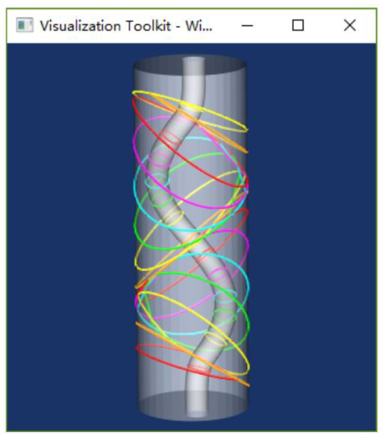And also, at each partitioning plane, the f_c values were all greater than il, implying that the inclination was not too large to hinder the support-free construction. 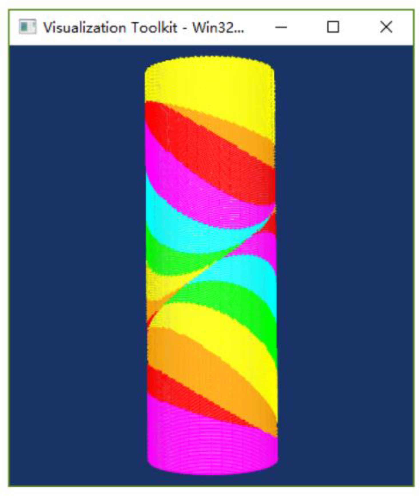The partitioning result is visualized in Figure 18, showing that the position and the direction of the partitioning planes changed with the variation in the guideline of the inner runner. The profile rings were constructed correctly, consistent with the actual situation, under the conditions of complex intersection among the partitioning planes and model. Figure 19 presents the slicing result. The slicing process was performed after the mentioned “top to bottom partitioning” process, and it can be seen from the result that no slice interference occurred in the end, and the slicing direction is the desired fabricating direction.

Note that Figure 19 only presents the partitioning result for considering the inner runner, but for some sub-models, further consideration of the outer surface was needed to achieve the non-support fabrication. The method for considering the outer surface is not discussed, because it has already been solved by various researchers mentioned in the introduction section.

7. Conclusions and Future Work

In this paper, a novel partitioning method for support-free fabrication models with an inner runner is proposed, and relative mathematical methods are presented. Analysis has been carried out for some varying parameters, and a program was coded in Python language and the VTK toolkit for visualization of the partitioning result. The analysis and verification indicated that the method was successful in partitioning the model for support-free construction of the inner runner. The achievements of this paper can be concluded as follows:

(1)

The proximity Φ_s affects the number of partitioning planes acquired, the accuracy of the partitioning plane’s directions, and the calculation time. A smaller Φ_s causes less time consumption, but will generate more planes with larger intersecting angles between the normals of the partitioning planes and the inner runner guideline direction.

(2)

The increment coefficient σ mainly affects the calculation time, where a greater σ will also reduce the time consumption, accelerating the converging speed. However, greater σ values will also bring iteration difficulties when approaching a greater Φ_s.

(3)

There is a turning point in the solution process of the algorithm. When the proximity Φ is less than or equal to a certain critical value, the increasing rate is significant (but gradually decreases) during the iteration. When Φ is greater than that critical value, the increasing rate of Φ will sharply decrease, and then the Φ value will increase slowly in each iteration step until the validation of Φ ≥ Φ_s. The critical value of Φ occurs at about the 1/4 of the total iteration steps needed for each plane.

(4)

During the whole solution process, the fc values are always less than il, implying that the planes generated by the proposed method certainly partition the model, avoiding too large tilting angles existing between the facets that approximate the inner runner surface and the guideline direction. Thus, support-free printing for the inner runner is possible.

In the future, more work considering real additive manufacturing processes will be carried out on this project, and the decision of the key parameter, the tilt limit il, will be investigated, depending on corresponding additive manufacturing process parameters and material characteristics.