Equilibrium Strategy of Production and Order in a Two-Echelon Supply Chain with Demand Information Updates and Capacity Restriction

Abstract

This paper studies production-and-order strategies under three production systems in which the supplier’s production quantity is constrained by the upfront preparations of capacity due to a long production season. The newsvendor-like retailer may make an advance order at the beginning of the production season, relying on early demand information, or a delay order at the end of the production season, depending on the updated demand information. In two special cases of perfect and imperfect demand information updates, this paper analytically derives the optimal decision equilibrium of a supplier-led Stackelberg game for three production-and-order strategies: (1) advance order under single regular production, (2) delay order under single emergency production and (3) delay order under two-mode production. In the case of perfect information updates, all three strategies likely become the equilibrium strategies that depend on the instant wholesale price and on the production cost for emergency production. In the case of imperfect information updates, the strategy of advance orders under regular production represents the unique equilibrium of the supply chain. Furthermore, the effect of general demand information updates on the equilibrium strategy is analyzed. Counterintuitively, the research results show that the retailer is more profitable with imperfect information updates than with perfect information updates when a high instant wholesale price is charged. In sharp contrast to previous studies, where the supplier always benefits from a two-mode production system due to its flexibility, our results indicate that the supplier would prefer a single regular production system when the production cost under emergency production is large, or the quality of demand information is high. Numerical examples verify our theoretical results.

1. Introduction

The mismatch between supply and demand leads to an increasing cost of inventory and/or stock-outs, which seriously damages supply chain performance. Traditional enterprises usually utilize historical data to forecast demand. However, since the market environment changes quickly, demand forecasts based on historical data may not be accurate [1,2,3]. For example, in the early 2000s, some high-tech enterprises declared bankruptcy due to sharp demand shortfalls [4]. Recently, with the rapid development of information technology, market information can easily be collected and employed for improving demand forecast accuracy [5]. For instance, the web logs of Amazon gather more than 30 GB of data every day to collect and analyze market consumption data [6]. Many fashion companies, such as Uniqlo, Zara and Topshop, have adopted big data technology to obtain updated demand information to make ordering more accurate decisions and improve channel performance. To better match supply and demand, downstream retailers prefer to postpone making their order decisions until more accurate demand information is available [7]. However, due to a long production lead time in fashion apparel and high-tech industries, the upstream supplier builds capacity prior to receiving final orders from the downstream retailer so as to provide timely order fulfilment. High demand uncertainty and short lifecycles increase the risk of surplus capacity for the supplier [8]. Hence, upstream suppliers prefer retailers to place full orders as early as possible. Such decision conflict between the supplier and retailer results in an inefficient supply chain, which has received considerable attention in the supply chain management literature and industrial practice.

Motivated by the abovementioned real business scenario, this paper studies the equilibrium strategy of production and ordering in a two-echelon supply chain with demand information updates and capacity restriction. The demand information can be updated during the supplier’s long production season. The retailer could order at the beginning of the production season using less accurate early demand information (i.e., advance order) or order at the beginning of the sales season using more accurate updated demand information (i.e., delay order). To induce the retailer to place orders as early as possible, the supplier offers a smaller wholesale price under an advance order (i.e., an advance wholesale price) than that under delay order (i.e., instant wholesale price). Under an advance order, the retailer takes all of the risk, while they could be charged a low advance wholesale price. On the contrary, under delay order, the retailer only takes part of the risk but will be charged a high instant wholesale price. To decide on a profit-maximizing ordering strategy, including ordering time selection and ordering quantity decision, the retailer has to evaluate the trade-off between a higher wholesale price and a lower market risk if delay order is available.

Furthermore, to match the supplier’s production and the retailer’s order, one of the approaches is to postpone some (or all) production until demand information is updated [9]. Many studies have categorized this approach into two-mode production systems, including regular mode and emergency mode [10,11,12]. Generally, the production cost in the regular mode is lower than that in the emergency mode. If the retailer chooses to order in advance, the supplier adopts the regular mode to produce goods according to a “make-to-order” policy. The supplier sets a lower advance wholesale price and takes a smaller production cost without any production risk. If the retailer chooses delay order, the supplier adopts the emergency mode or two-mode production. It is worth pointing out that since production lead time is long, the supplier has to prepare its capacity in advance. Hence, the production quantity in the emergency mode is constrained by the initially prepared capacity. Compared with the regular mode, the supplier faces a higher instant wholesale price and a bigger emergency production cost, and may bear some over-capacity risk. Similarly, to determine a profit-maximizing production strategy, including production time selection and production quantity decision, there exists a trade-off for the supplier between a higher wholesale price and a larger market risk under the emergency mode.

Our research is significant in that this paper studies supply chain management by considering both demand information updates and capacity restriction. As shown in the literature review (Section 2), previous studies show that when the wholesale price is constant before or after demand information updates, the retailer always benefits from order flexibility, whereas the supplier only benefits when the level of flexibility is small [13,14]. However, this paper assumes that the wholesale price is variable. Additionally, existing papers have shown that the emergency mode always benefits the supply chain without capacity restriction [15,16]. The difference is that this paper has a capacity restriction in the emergency mode. Considering a two-echelon supply chain composed of a supplier with capacity restriction and a retailer that can update demand information, we address the following questions:

(1)

What is the optimal production-and-order strategy in a two-echelon supply chain with demand information updates and capacity restrictions?

(2)

How are the decisions and performance of the supply chain affected by the variable wholesale prices and the quality of demand information updates?

(3)

Is there an equilibrium strategy of production and order among the supply chain members?

To answer above questions, this paper constructs a two-stage dynamic-game theoretical model with demand information updates and capacity restriction. Meanwhile, we consider three production and ordering strategies: (1) Strategy 1: the retailer chooses to make an advance order and the supplier adopts the regular mode; (2) Strategy 2: the retailer chooses to delay placing orders and the supplier adopts the emergency mode; (3) Strategy 3: the retailer chooses to make a delay order and the supplier adopts a two-mode production system. We have technically derived the supplier’s optimal production strategy policy and the retailer’s optimal ordering strategy under strategies 1–3, respectively. By comparing the supply chain members’ expected profits under above three strategies, the study shows that there exists a unique equilibrium strategy of production and ordering when demand information updates are imperfect or perfect. Furthermore, a numerical simulation is executed to verify that the unique equilibrium strategy still exists when demand information updates are general. This paper’s objective is to technically analyze the equilibrium strategy of production and order in a two-echelon supply chain with demand information updates and capacity restriction. Based on the obtained theoretical results, this study offers valuable insights into how firms could manage the supply chain’s production and order when facing capacity restriction in the presence of demand information updates.

Our study contributes to the literature as follows. First, this paper develops a two-stage Stackelberg game model to derive the supplier’s optimal production strategy policy and the retailer’s optimal ordering strategy with demand information updates and capacity restriction. Second, this paper investigates the effect of demand information update quality and wholesale price effects on the supply chain members’ optimal production and order strategy selection. Contrary to previous studies, when the wholesale prices are variable, the demand information updates benefit the retailer only when instant wholesale price is at a low level. Interestingly, as long as the instant wholesale price is at a high level, the supplier always benefits from demand information updates. Third, this paper further proves that there exists a unique equilibrium strategy of production and ordering under certain conditions. Therefore, our study offers valuable insights into how enterprises could manage the supply chain with demand information updates and capacity restriction.

The remainder of this paper is organized as follows. Section 2 reviews the related literature. Section 3 gives the model description. Section 4 studies the optimal production and order decisions under three strategies. Section 5 provides strategy selection and equilibrium analysis in two special cases. Section 6 conducts a numerical simulation with a general demand signal. Section 7 gives the conclusion and management insights. For clarity of exposition, all of the proofs are presented in Appendix A.

2. Literature Review

This paper mainly contributes to two streams of related research in supply chain management: production and ordering strategy with demand information updates and production mode selection in inventory models. In what follows, a concise review and further discussion is presented to highlight the differences and similarities between this study and the reviewed literature.

2.1. Production and Ordering Strategy with Demand Information Updates

Production and ordering strategies with demand information updates have received a great deal of attention from researchers and practitioners in various settings. There are two main research directions in the literature. In the first direction, demand information updates occur during the sales season with a two-stage correlated-demand model. The retailer can utilize the realized demand from the first stage to update the demand forecast for the second stage [9,10,14,16,17,18,19,20,21,22,23,24]. For example, [10] studied the role of options in a two-period model with correlated demand. They illustrated how options provide flexibility to respond to market changes in the second period. The authors of [14] proposed an improved revenue-sharing contract in a two-echelon supply chain with two ordering opportunities. In [9], the authors analyzed a two-stage supply chain model in which a reactive production exists in Stage 2 after demand information is updated, but production capacity must be prepared in Stage 1. The authors of [20] studied a two-stage inventory management problem with demand information updates and a capital-constrained retailer. They presented a recourse approach to solve the two-stage optimization problem and derive the optimal inventory/financing policies.

Furthermore, in the second direction, demand information updates occur in the production season. The retailer can update the demand forecast by observing new market signals during the production season [3,8,15,25,26,27,28,29,30,31,32,33,34,35,36,37,38]. For example, [31] studied the optimal ordering policy for a retailer who has two order instants before and after demand information updates with an uncertain cost. They characterized the conditions in which it is optimal for the retailer to delay its order until the second instant. In [25], the authors considered a two-stage dynamic optimization problem with a Bayesian update. They used dynamic programming methods to derive the retailer’s optimal order strategy. In [28] and [29], the authors proposed a three-parameter risk and profit-sharing contract to coordinate the supply chain with demand information updates and price-dependent demands. The authors of [36] analyzed a two-stage order model with capital constraints and demand forecast update. They found that the optimal policy is characterized by targeted safety capital. In [26], the authors studied the fashion quick response program with social media observations, demand forecast updating and a boundedly rational retailer. He found that the likelihood of good product reviews on social media plays a critical role in affecting the value of quick response, and its effect is mediated by the fashion retailer’s prior attitudes towards the market demand. The authors of [3] investigated a single two-echelon supply chain consisting of a supplier and a capital-constrained retailer. They proved the existence of optimal equilibrium solutions under both an advance order and regular order strategies. In [37], authors proposed an option buyback hybrid contract to achieve perfect coordination for a two-echelon supply chain under demand information updates. The authors of [33] addressed the optimal production and procurement planning in a random yield supply chain with perfect and imperfect demand information updating. They found that the pure option contract can coordinate the supply chain only when demand information is updated and perfect, while the option contract with a buyback mechanism can coordinate the supply chain only when demand information is updated and imperfect. In [32], the authors analyzed incentive strategies of low-carbon supply chains by considering the information update of low-carbon preferences. They designed an optimal carbon reduction model for the government and proved that cooperation of profit-driven supply chain members improves not only their profits but also carbon reduction efficiency. The authors of [38] investigated the impact of information updates on product quantity, information rent, and the profit of the supplier. They found that the multiperiod incentive mechanism under limited commitment has an intertemporal effect compared to the incentive mechanism under symmetric information and full commitment due to dishonest reporting by retailers.

In addition, the first direction is reasonable for products with a long selling period, while the second direction is acceptable for products with a short life cycle, and this paper belongs to the latter. Prior works showed that demand information updates always beneficial to the retailer but may hurt the supplier. However, this paper develops game models to derive the retailer’s optimal ordering strategy and the supplier’s optimal production strategy with or without demand information updates. When the wholesale prices are variable, our study finds that the retailer benefits from demand information updates only when the wholesale price under delay orders is lower. However, the supplier benefits from demand information updates as long as the wholesale price under delay orders is large enough.

2.2. Production Mode Selection in Inventory Models

Many studies in the literature have investigated two-mode production systems in inventory models in which both purely regular production modes and purely emergency production modes are available [9,10,11,13,15,35,39,40,41,42,43,44,45,46,47,48,49,50,51,52]). For example, [15] developed supply contracts to design proper a coordination mechanism for forecast information and production decisions in a two-mode production environment. The author also examined whether the coordination conditions under two-mode production systems ensured a Pareto optimal solution with respect to two traditional production settings. The authors of [43] studied a simple supply chain with one supplier and one retailer where there is a random yield production and uncertain demand. They proposed several risk-sharing contracts that distribute the random yield risk among parties and evaluate the supply chain performance levels. In [41], the authors analyzed three types of supply contracts between a supplier and a retailer in which the purchased item can be shipped to the retailer on an expedited basis at no extra cost once stock-out occurs. The authors of [52] developed a concept called EUOS (expected unit opportunity saving) to examine the expected benefit received per unit of the option under different market scenarios. Most prior works have shown that the mix-mode production system is more profitable than the single-mode production systems (purely regular production mode and purely emergency production mode). However, our study proves that not only the mix-mode production system but also the single-mode production models could be optimal production strategies under certain conditions. In [40], the authors studied inventory and production problems in a sustainable green supply chain by constructing a multi-objective optimization model. They focused on the impact of holding costs on green inventory decisions and system performance. [48] investigated the fixed costs of ordering items and the optimality of $\left(s,S\right)$ policies for various inventory models. To explore future research extensions and directions, they reviewed the extensive literature on continuous-time models over seven decades. The authors of [46] studied the optimal production strategy and the optimal pricing strategy in a festival food supply chain under two production modes. They designed a risk-sharing mechanism for an option contract to coordinate such a supply chain under certain conditions. In [50], the authors proposed a heuristic algorithm approach to solve an MTO–MTS (Make-to-Order/Make-to-Stock) production system where finished and semi-finished products are produced to meet customer demands. They verified the effectiveness of the method by simulating it with multiple data sets from a steel plant. [47] investigated comprehensive joint decision making consisting of technology selection, production planning and pricing decisions in a two-echelon supply chain considering both carbon emission tax and subsidy offered by the local government. They developed a nested genetic algorithm (NGA) to solve the Stackelberg game model and shed light on several important managerial implications for the manufacturer. The authors of [44] studied the optimal policy that minimizes cost by exploring two extreme advance delivery information regimes, including full delivery information and partial delivery information in an EOQ model. They found that advanced information can directly reduce operating costs by reducing planning uncertainty. In [42], the authors introduced a new capital equilibrium strategy that can effectively switch the control of system capital costs, ultimately helping to reduce costs and enhance system stability.

Based on the above discussion, many studies of inventory models which utilize the regular mode, emergency mode or both modes to meet uncertain market demands. These studies imply the assumption of constant demand fluctuations, and the problems studied are also limited to the single-period decision environment. However, with the rapid development of information technology, more and more enterprises are trying to use emerging digital technologies to collect and update demand information so as to respond quickly to market changes. Therefore, this paper studies the production and order strategy for a two-echelon supply chain in the context of demand information updates. Compared with traditional research, there are two major changes: first, the demand fluctuation is changing. In particular, demand uncertainty continues to decrease as demand information is updated. Second, the decision making of supply chain members under the demand information update is a two-stage dynamic process and will be more complex.

2.3. Research Gap and Contribution

Table 1. Summary of the related literature.

Literatures	Wholesale Price	Production Mode	Capacity Restriction	Demand Information Updates
[31]	Variable	Regular	No	Yes
[10]	Variable	Two	No	Yes
[28,29]	Constant	Regular	Yes	Yes
[14,16]	Constant	Regular	No	Yes
[41]	Variable	Two	No	No
[36]	Variable	Regular	Yes	Yes
[45]	Constant	Two	No	No
[52]	Variable	Regular	Yes	Yes
[9]	Variable	Emergency	Yes	Yes
[3]	Variable	Regular	No	Yes
[37]	Constant	Regular	Yes	Yes
[33]	Constant	Two	No	Yes
[50]	Constant	Two	No	No
[47]	Variable	Regular	No	No
This paper	Variable	Two	Yes	Yes

summarizes the related research and presents a comparative analysis. As shown in Section 2.1 and Section 2.2, this paper is closest to [3,9,33], but there are still several major differences. It is worth noting that most studies focus on the impact of demand information updates on the retailer’s ordering strategy, while ignoring the changes in the supplier’s production decisions after demand information updates. In this paper, the retailer can order before or after the demand information is updated, while the supplier’s production can adopt the regular mode, the emergency mode, or two-mode of production system. Our study attempts to explore the interaction between the retailer’s order and the supplier’s production under demand information updates. Furthermore, compared with [3,9,33], our study mainly focuses on how the supplier’s various production mode selection with capacity restrictions affects the retailer’s order strategy with demand information updates. More importantly, this paper not only studies the optimal production and ordering decisions in a two-echelon supply chain with capacity restriction and demand information updates, but also the equilibrium strategy of production and ordering as well as the role of variable wholesale prices and the quality of demand information updates in a supply chain member’s strategy selection.

This paper contributes to the literature in the following aspects: First, it develops a game-theoretic decision making model of the supplier’s production and the retailer’s order with capacity restrictions and demand information updates. In contrast, the existing literature mostly assumes that there is sufficient capacity, but demand information is not updated. Second, it characterizes the optimal equilibriums of production and order strategy between the supplier and retailer under perfect and imperfect demand information updates, respectively. Unlike the existing literature that only focuses on a single production mode, this paper explores how the supplier adopts the regular mode, emergency mode, and two-mode systems to deal with a retailer’s orders with demand information updates. Third, it examines the impact of demand information update quality and wholesale price changes on supply chain members’ selection of production and ordering strategy; these theoretical findings may have some meaningful managerial implications for inventory management and operation decisions of supply chain enterprises.

3. Model Description

This paper considers a two-echelon supply chain consisting of a single retailer (“he”) and a single supplier (“she”). As the production lead time is long, the demand information can be updated during the production season. For the retailer, there is only one opportunity to order, either order before demand information updates without new market signal (hereafter, advance order for brevity) or order after demand information updates with new market signal (hereafter, delay order for brevity). On the other hand, for the supplier, if the retailer chooses to make an advance order, the supplier would produce in the regular mode at a cheap production cost following a “make-to-order” policy. In this case, the retailer takes all the risk of overordering. If the retailer chooses to make a delay order, the supplier needs to prepare capacity in advance. For this case, the retailer could transfer part of overordering risk to the overproduction risk for the supplier. To reduce production risk and fulfill the order, the supplier may produce in the emergency mode at an expensive production cost or in a production system that combines two-mode (regular mode and emergency mode). Hence, there will exist three possible production and order strategies, which are shown in Figure 1.

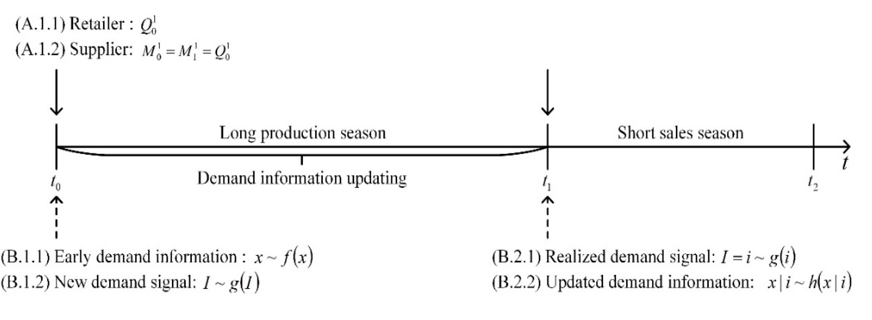
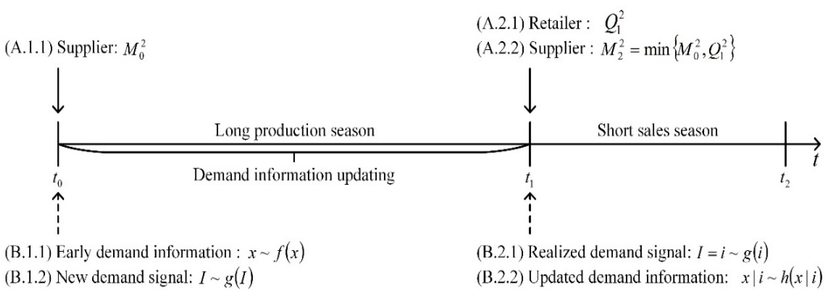
3.1. The Progress of Demand Information Updates

The supply chain members face a stochastic market demand, which can be updated by market signals observed during a long production season. Following [18], the process of demand information updates is expressed as follows: At the beginning of the production season (i.e.,$t=t_0$), the early demand information $x$ has a prior probability distribution $F\left(x\right)$ and a density function $f\left(x\right)$. During a long production season (i.e.,$t=t_0~t_1$), the retailer will collect new market signal $I$ by observing changes in consumers, where $G\left(I\right)$ and $g\left(I\right)$ denote the marginal distribution and density of $I$, respectively. At the end of the production season (i.e.,$t=t_1$), the new market signal $I$ realized as $i$. The updated demand information $x|i$ has a posterior distribution $H\left(x|i\right)$ and density function $h\left(x|i\right)$.

Many conjugate distributions can satisfy the above assumptions, such as Uniform-Uniform, Uniform-Pareto, Gamma-Poisson, and Normal-Normal distributions. Without loss of generality, assume that the joint distribution of the realized demand signal $i$ and the early demand information $x$, $\phi \left(i,x\right)$, is a bivariate normal distribution with means $m$ and $\mu$, standard deviations $s$ and $\sigma$, and the correlation coefficient $\rho$. Following [53], $x|i$ is normally distributed with ${\mu }^{\prime }$ and ${\sigma }^{\prime }$,

$${\mu }^{\prime }=\mu +\frac{\rho \left(i-m\right)\sigma }{s} \mathrm{and} {\sigma }^{\prime }=\sigma \sqrt{1-{\rho }^2}.$$

(1)

where $\rho$ represents the quality of demand information updates. The variance of $x$ and $x|i$ is $var\left(x\right)=\sigma$ and $var\left(x|i\right)={\sigma }^{\prime }$ respectively. Since $0\le \rho \le 1$, then $var\left(x|i\right)\le var\left(x\right)$, which shows that the retailer can obtain a more accurate demand information through demand information updates. Furthermore, there exist two special cases of the quality of demand information updates as follows.

(1) $\rho =0$, $var\left(x|i\right)=var\left(x\right)$, which indicates that the realized demand signal $i$ does not have any impacts on the demand uncertainty. This is called an imperfect signal.

(2) $\rho =1$, $var\left(x|i\right)=0$, which indicates that the market demand can be completely determined by the latest demand signal $i$. This is called a perfect signal.

Normally, $0<\rho <1$ indicates the general demand signal.

3.2. Costs

Due to a long production lead time, the supplier has to build capacity beforehand at a unit cost $c_0$. With the capacity prepared in advance, the supplier has two production opportunities. She can produce via the regular mode with a cheap unit cost $c_1$ at the beginning of the production season. In addition, she can produce via the emergency mode at an expensive unit cost $c_2$ at the beginning of the sales season. With a two-mode production system, the supplier offers two wholesale prices $w_1$ and $w_2$ to the retailer. Assume that $c_1\le c_2$ and $w_1\le w_2$ which are exogenously determined. Such assumptions create two trade-offs for both the supplier and the retailer. To determine the profit-maximizing order strategies, the retailer has to evaluate the trade-off between a more accurate forecast and a higher unit cost after demand information updates. Similarly, the supplier has to evaluate the trade-off between an overcapacity risk and a higher wholesale price after demand information updates.

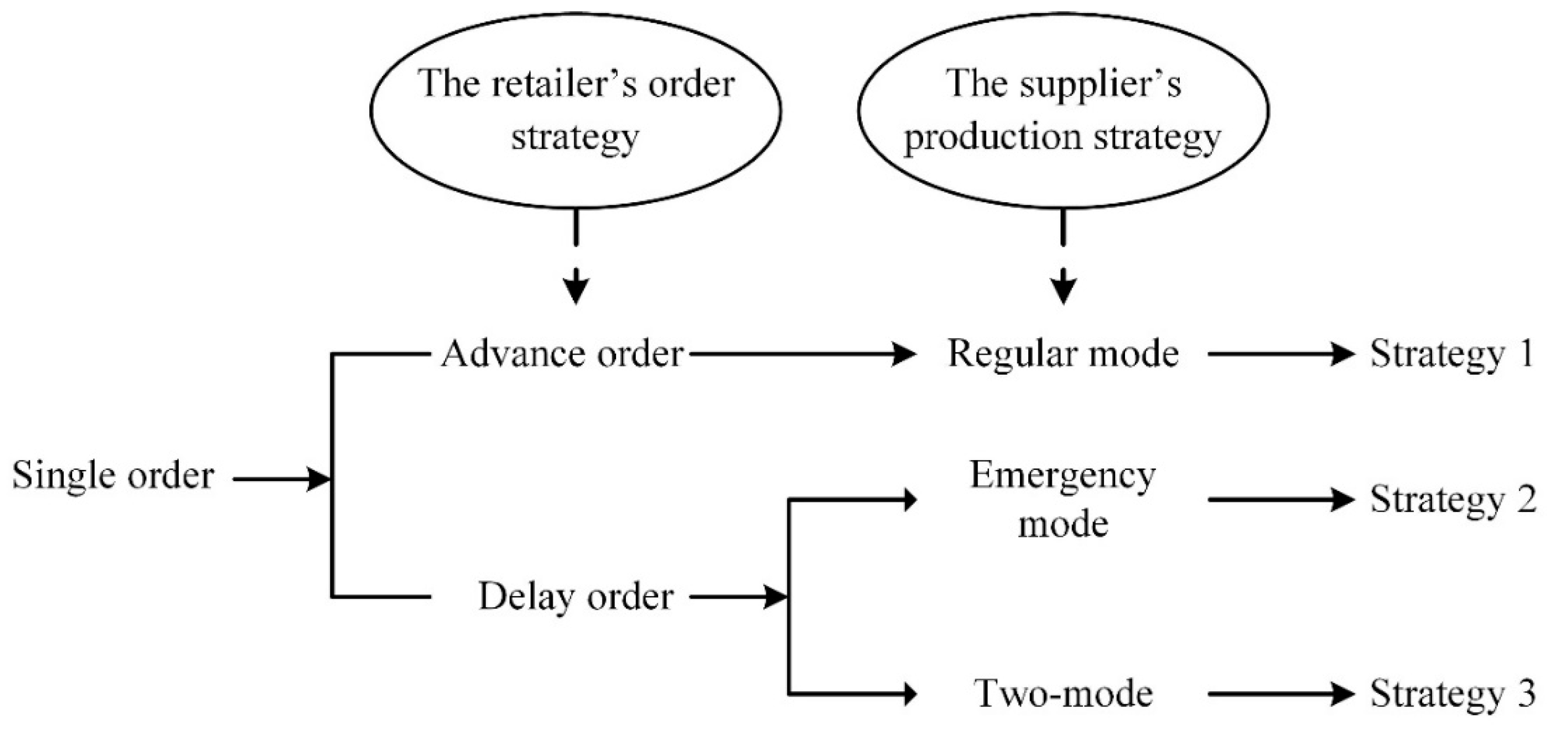
3.3. The Decision Progress in Three Strategies

The decision progress of three production and order strategies are expressed as follows, respectively.

(1) Strategy 1 (Advance order with the regular mode): As shown in Figure 2, at $t=t_0$, the retailer first determines the order quantity $Q_0^1$ based on the early demand information $x$ at unit wholesale price $w_1$. Then, the supplier prepares capacity $M_0^1$ at unit cost $c_0$ and produces $M_1^1$ in the regular mode at unit cost $c_1$. By adopting a “make-to-order” policy, we obtain $M_0^1=M_1^1=Q_0^1$.

(2) Strategy 2 (Delay order with the emergency mode): As shown in Figure 3, at $t=t_0$, the supplier first prepares capacity $M_0^2$ based on the early demand information $x$ at unit cost $c_0$. Then, at $t=t_1$, the retailer determines order quantity $Q_1^2$ based on the updated demand information $x|i$ at unit wholesale price $w_2$. To provide timely order fulfilment, the supplier will produce $M_2^2$ in the emergency mode at unit cost $c_2$. Due to the initial prepared capacity limit, we obtain $Q_1^2=M_2^2\le M_0^2$.

(3) Strategy 3 (Two-mode of delayed order production system): As shown in Figure 4, at $t=t_0$, according to the early demand information $x$, the supplier prepares capacity $M_0^3$ at unit cost $c_0$ and produces $M_1^3$ in the regular mode at unit cost $c_1$. At $t=t_1$, the retailer determines order quantity $Q_1^3$ based on the updated demand information $x|i$ at unit wholesale price $w_2$. If $Q_1^3>M_1^3$, then the supplier produces $M_2^3$ in the emergency mode at unit cost $c_2$ in the case of shortage. In addition, due to initial prepared capacity limit, we obtain $Q_1^3\le M_0^3$.

3.4. Notation and Assumption

After considering the existing literature and realistic situations, some research assumptions for demand information updates are presented as follows: (1) $i$ is expressed in the same unit as total demand with a lower support $i_{min}=0$ [31]; (2) the demand information updates make the demand forecast more accurate than the original forecast [28,29]; (3) the random variable $x|i$ is increasing in $i$ [8]; (4) when $i_1<i_2$, the cumulative distribution $H\left(x|i\right)$ for $x$ given $i$ satisfies $H\left(x|i_1\right)\ge H\left(x|i_2\right)$ [52]; (5) the demand information and the conditional distribution of the final demand is symmetric for all supply chain parties [28,29,52]; and (6) all distributions are continuous, differentiable, invertible and independent of the cost and price [30].

Furthermore, to avoid meaningless situations and non-trivial cases, similarly to [33], assume that $p>w_2>w_1>c_2>c_1>c_0>v_0>v_s>v_r$, where $p$ is retail price, and $v_0$, $v_s$ and $v_r$ are the salvage values of unused capacity, unused capacity and unsold product, respectively. Without a loss of generality, the holding cost and penalty cost are assumed to be zero [51].

For simplicity, the notation is summarized in

Table 2. Notations and explanations.

Notation	Explanation
$x$	Early demand information
$I$	New demand signal
$i$	Realized demand signal
$x|i$	Updated demand information
$p$	Retail price
$c_0$	Capacity cost
$c_1$	Production cost in the regular mode
$c_2$	Production cost in the emergency mode
$v_0$	Salvage value of unused capacity
$v_s$	Salvage value of unused product
$v_r$	Salvage value of unsold product
$w_1$	Wholesale price in an advance order
$w_2$	Wholesale price in a delay order
$Q_0^k$	Advance order quantity in strategy $k$, where $k=1$, 2, 3 (decision variable)
$Q_1^k$	Delay order quantity in strategy $k$, where $k=1$, 2, 3 (decision variable)
$M_0^k$	Capacity quantity in strategy $k$, where $k=1$, 2, 3 (decision variable)
$M_1^k$	Regular production quantity in strategy $k$, where $k=1$, 2, 3 (decision variable)
$M_2^k$	Emergency production quantity in strategy $k$, where $k=1$, 2, 3 (decision variable)
${\pi }_r^k\left(·\right)$	Expected profit of the retailer in strategy $k$, where $k=1$, 2, 3
${\pi }_s^k\left(·\right)$	Expected profit of the supplier in strategy $k$, where $k=1$, 2, 3
$f\left(·\right)$, $F(·)$	Probability density and distribution function of $x$
$g(·)$, $G(·)$	Probability density and distribution function of $I$
$h(x|i)$, $H(x|i)$	Probability density and distribution function of $x|i$ when $I=i$

.

4. The Decision Analysis

4.1. Strategy 1: Advance Order with Regular Mode

In this case, the retailer faces a newsvendor problem with uncertain market demand, while the supplier faces a production problem with deterministic demand from the retailer. Hence, the retailer takes all demand risk and the supplier takes no demand risk. Similarly to [3], let ${\pi }_r^1\left(Q_0^1\right)$ be the retailer’s expected profit function in strategy 1. Then, the retailer’s problem is expressed as optimization problem (P1).

$$(\mathrm{P}1): \underset{Q_0^1}{\mathrm{Maximize}}{\pi }_r^1\left(Q_0^1\right)$$

$$\mathrm{s}\mathrm{u}\mathrm{b}\mathrm{j}\mathrm{e}\mathrm{c}\mathrm{t} \mathrm{t}\mathrm{o} Q_0^1\ge 0,$$

where ${\pi }_r^1\left(Q_0^1\right)=E_{\left\{x\right\}}\left\{p\min \left\{x,Q_0^1\right\}-w_1{Q}_0^1+v_r{\left(Q_0^1-x\right)}^{+}\right\}$. Then, proposition 1 shows the retailer’s optimal order quantity $Q_0^{1\mathrm{*}}$ in strategy 1.

Proposition 1.

${\pi }_r^1\left(Q_0^1\right)$ is concave in $Q_0^1$ and $Q_0^{1*}=F^{-1}\left(\frac{p-w_1}{p-v_r}\right)$.

When the retailer chooses to order in advance without demand information updates, Proposition 1 shows that the retailer’s optimal advance order quantity depends on the advance wholesale price, retail price, and the salvage value of unsold products. This is consistent with classical research results in supply chain management. Based on the optimal $Q_0^{1*}$, the retailer’s expected profit in strategy 1 is

$${\pi }_r^1=\left(p-w_1\right)Q_0^{1\mathrm{*}}-\left(p-v_r\right){\int }_0^{Q_0^{1\mathrm{*}}}F\left(x\right)dx.$$

(2)

Under strategy 1, the supplier prepares capacity $M_0^1$ and produces $M_1^1$ in the regular mode with $M_0^1=M_1^1=Q_0^{1*}$. Then, the supplier’s expected profit function is

$${\pi }_s^1\left(M_0^1,M_1^1\right)=w_1{Q}_0^1-c_0{M}_0^1-c_1{M}_0^1.$$

Since the supplier adopts “make-to-order” policy, then $M_0^{1*}=M_1^{1*}=Q^{1*}$. Hence, the supplier’s expected profit in strategy 1 is

$${\pi }_s^1=\left(w_1-c_0-c_1\right)Q_0^{1\mathrm{*}}.$$

(3)

4.2. Strategy 2: Delay Order with Emergency Mode

In this case, the retailer faces a newsvendor problem with demand information updates, while the supplier faces a production problem with uncertain capacity from the retailer. Compared with strategy 1, part of the demand risk is transferred from the retailer to the supplier in strategy 2. Hence, the retailer takes overstock risk and the supplier bears overcapacity risk due to demand uncertainty. The backward induction is utilized to solve the supply chain members’ problem.

First, at $t=t_1$, given $M_0^2$ and $I=i$, let ${\pi }_r^2\left(M_0^2,i;Q_1^2\right)$ be the retailer’s expected profit function in strategy 2. Then, the retailer’s problem is expressed as optimization problem (P2).

$$(\mathrm{P}2): \underset{Q^2}{\mathrm{Maximize}}{\pi }_r^2\left(M_0^2,i;Q_1^2\right)$$

$$\mathrm{s}\mathrm{u}\mathrm{b}\mathrm{j}\mathrm{e}\mathrm{c}\mathrm{t} \mathrm{t}\mathrm{o} 0\le Q_1^2\le M_0^2,$$

where ${\pi }_r^2\left(M_0^2,i;Q_1^2\right)=E_{\left\{x|i\right\}}\left\{p\min \left\{x,Q_1^2\right\}-w_2{Q}_1^2+v_r{\left(Q_1^2-x\right)}^{+}\right\}$. Let $Q_1^2|i=H^{-1}\left(\frac{p-w_2}{p-v_r}|i\right)$, where $H^{-1}\left(·|i\right)$ is the inverse function of $H\left(·|i\right)$. Then, proposition 2 establishes the retailer’s optimal order quantity $Q_1^{2\mathrm{*}}$ in strategy 2.

Proposition 2.

Given $M_0^2$, $I=i$ in sales season, ${\pi }_r^2\left(M_0^2,i;Q_1^2\right)$ is concave in $Q_1^2$, and $Q_1^{2*}=\mathit{min}\left\{Q_1^2|i, M_0^2\right\}=\left\{\begin{array}{c}{Q}_1^2|i, if i\le i_{M_0^2},\\ M_0^2, if i>i_{M_0^2},\end{array}\right.$ where $i_{M_0^2}$ satisfies $Q_1^2|i_{M_0^2}=M_0^2$.

Proposition 2 shows that when the retailer chooses to make a delay order when demand information is updated, the retailer’s optimal delay order quantity depends not only on the realized demand signal but also on the supplier’s initial capacity restriction. It indicates that the supplier’s advance capacity decision and updated demand information constrain the retailer’s ordering behavior. This also implies that the value of the retailer’s demand information update will be limited due to capacity restrictions. There exists a signal threshold $i_{M_0^2}$ such that the retailer’s optimal delay order quantity just equals the supplier’s initial prepared capacity quantity. From Proposition 2, when the realized demand signal is smaller than the information threshold value, i.e., $i\le i_{M_0^2}$, the supplier’s capacity is sufficient to satisfy the retailer’s order, i.e., $Q_1^{2\mathrm{*}}=Q_1^2|i\le M_0^2$. By adopting a “make-to-order” policy, the supplier’s optimal production quantity is $M_2^{2\mathrm{*}}=Q_1^2|i$. For this case, the expected profit of the retailer and the supplier is

$${\pi }_r^2\left(M_0^2,i;Q_1^2|i\right)=\left(p-w_2\right)Q_1^2|i-\left(p-v_r\right){\int }_0^{Q_1^2|i}F\left(x|i\right)dx,$$

(4)

$${\pi }_s^2\left(M_0^2,i;Q_1^2|i\right)=\left(w_2-c_2\right)Q_1^2|i+v_0\left(M_0^2-Q_1^2|i\right).$$

(5)

However, when the realized demand signal is larger than the threshold value, i.e., $i>i_{M_0^2}$, then the supplier’s capacity is insufficient to satisfy the retailer’s order, i.e., $Q_1^2|i>M_0^2$. Since ${\pi }_r^2\left(M_0^2,i;Q^2\right)$ is unimodal, then $Q_1^{2\mathrm{*}}=M_0^2$. The supplier’s optimal production quantity in the emergency mode is $M_2^{2\mathrm{*}}=M_0^2$. In this case, the expected profits of the retailer and the supplier at the beginning of sales season are

$${\pi }_r^2\left(M_0^2,i;M_0^2\right)=\left(p-w_2\right)M_0^2-\left(p-v_r\right){\int }_0^{M_0^2}F\left(x|i\right)dx,$$

(6)

$${\pi }_s^2\left(M_0^2,i;M_0^2\right)=\left(w_2-c_2\right)M_0^2.$$

(7)

Next, at $t=t_0$, let ${\pi }_s^2\left(M_0^2\right)$ be the supplier expected profit function in strategy 2. Then, the supplier’s problem is expressed as optimization problem (P3).

$$(\mathrm{P}3): \underset{M_0^2}{\mathrm{Maximize}}{\pi }_s^2\left(M_0^2\right)$$

$$\mathrm{s}\mathrm{u}\mathrm{b}\mathrm{j}\mathrm{e}\mathrm{c}\mathrm{t} \mathrm{t}\mathrm{o} M_0^2\ge 0$$

(P3)

where ${\pi }_s^2\left(M_0^2\right)=-c_0{M}_0^2+{\int }_0^{i_{M_0^2}}{\pi }_s^2\left(M_0^2,i;Q^2|i\right)dG\left(i\right)+{\int }_{i_{M_0^2}}^{+\mathrm{\infty }}{\pi }_s^2\left(M_0^2,i;M_0^2\right)dG\left(i\right)$.

Following the proposition gives the supplier’s optimal capacity quantity in strategy 2.

Proposition 3.

${\pi }_s^2\left(M_0^2\right)$ is concave in  $M_0^2$, and $M_0^{2*}$ satisfies $G\left(i_{M_0^{2*}}\right)=\frac{w_2-c_2-c_0}{w_2-c_2-v_0}$.

Proposition 3 shows that the supplier’s optimal capacity quantity not only depends on the initial capacity cost but is also influenced by the emergency production cost. Following Proposition 3, the retailer’s realized optimal order in strategy 2 is $Q^{2\mathrm{*}}=\mathit{min}\left\{Q_1^2|i,M_0^{2\mathrm{*}}\right\}$, and his expected profit at the beginning of the sales season is

$$\begin{array}{c}{\pi }_r^2={\int }_0^{i_{M_0^{2*}}}\left[\left(p-w_2\right)Q_1^2|i-\left(p-v_r\right){\int }_0^{Q_1^2|i}H\left(x|i\right)dx\right]dG\left(i\right)+{\int }_{i_{M_0^{2*}}}^{+\infty }[(p-\\ w_2)M_0^{2*}-\left(p-v_r\right){\int }_0^{M_0^{2*}}H\left(x|i\right)dx]dG\left(i\right).\end{array}$$

(8)

Similarly, the supplier’s expected profit in strategy 2 is

$$\begin{array}{c}{\pi }_s^2=-c_0{M}_0^{2*}+{\int }_0^{i_{M_0^{2*}}}\left[\left(w_2-c_2\right)Q_1^2|i+v_0\left(M_0^{2*}-Q_1^2|i\right)\right]dG\left(i\right)+\\ {\int }_{i_{M_0^{2*}}}^{+\infty }\left[\left(w_2-c_2\right)M_0^{2*}\right]dG\left(i\right).\end{array}$$

(9)

4.3. Strategy 3: Delay Order with Two-Mode Production

In this case, the retailer still faces a newsvendor problem with demand information updates, while the supplier faces a two-stage production problem with uncertain demand from the retailer. The retailer’s order decision in strategy 3 is consistent with his counterpart in strategy 2. However, the supplier prepares capacity and produces using a two-mode production system to fulfill the retailer’s order. Compared with strategy 1 or 2, the supplier takes both overcapacity risk and overproduction risk in strategy 3. Hence, this paper further studies the supplier’s optimal production decision in the two-mode production system.

First, at $t=t_1$, given $M_0^3$, $M_1^3$, and $I=i$, it is optimal for the retailer to order $Q_1^3$, then there exist three scenarios associated with the supplier’s emergency production quantity $M_2^3$ as follows: (1) If $Q_1^3\le M_1^3\le M_0^3$, that is, the regular production quantity is enough to satisfy the retailer’s order quantity, then the emergency production is $M_2^3=0$, the unused product in the regular mode is $M_1^3-Q_1^3$, and the unused capacity is $M_0^3-M_1^3$; (2) If $M_1^3\le Q_1^3\le M_0^3$, that is, the regular production quantity is not enough but initial capacity quantity is sufficient to satisfy the retailer’s order quantity, then the emergency production is $M_2^3=Q_1^3-M_1^3$, the unused product is 0, and the unused capacity is $M_0^3-Q_1^3$; (3) If $M_1^3\le M_0^3\le Q_1^3$, that is, both the regular production quantity and initial capacity quantity is sufficient to satisfy the retailer’s order quantity, then the emergency production is $M_2^3=M_0^3-M_1^3$, the unused product is 0, and the unused capacity is 0. Taking the above three cases into consideration, the supplier’s expected profit in strategy 3 at the beginning of the sales season is given by

$$\begin{array}{c}{\pi }_s^3\left(M_0^3,M_1^3,i;M_2^3\right)=w_2{Q}_1^3-c_2{\left[\min \left\{M_0^3, Q_1^3\right\}-M_1^3\right]}^{+}+v_0[M_0^3-\\ {\max \left\{M_1^3,Q_1^3\right\}]}^{+}+v_s{\left(M_1^3-Q_1^3\right)}^{+}.\end{array}$$

(10)

where the first term is revenue from selling products, the second term is production cost in the emergency mode, the third term is the salvage value of unused capacity, and the fourth term is the salvage value of unused product.

For the retailer, the decision making at the beginning of the sales season is identical to strategy 2 except for the capacity quantity, which should be replaced by $M_0^3$. Let $Q_1^3|i=Q_1^2|i=H^{-1}\left(\frac{p-w_2}{p-v_r}|i\right)$. Then, the retailer’s optimal order quantity at $t=t_1$ in Strategy 3 is $Q_1^{3*}=\min \left\{Q_1^3|i, M_0^3\right\}=\left\{\begin{array}{c}{Q}_1^3|i, if i\le i_{M_0^3},\\ M_0^3, if i\ge i_{M_0^3},\end{array}\right.$ where $i_{M_0^3}$ satisfies $Q_1^3|i_{M_0^3}=M_0^3$. Similarly, the expected profit of the retailer is

$${\pi }_r^3\left(M_0^3,i;Q_1^{3*}\right)=\left\{\begin{array}{cc}{\pi }_r^3\left(M_0^3,i;Q_1^3|i\right),& if i\le i_{M_0^3},\\ {\pi }_r^3\left(M_0^3,i;M_0^3\right),& if i\ge i_{M_0^3},\end{array}\right.$$

(11)

where

$${\pi }_r^3\left(M_0^3,i;Q_1^3|i\right)=\left(p-w_2\right)Q_1^3|i-\left(p-v_r\right){\int }_0^{Q_1^3|i}H\left(x|i\right)dx,$$

(12)

$${\pi }_r^3\left(M_0^3,i;M_0^3\right)=\left(p-w_2\right)M_0^3-\left(p-v_r\right){\int }_0^{M_0^3}H\left(x|i\right)dx.$$

(13)

With the optimal order quantity $Q_1^{3*}$, following [50], there exist two threshold values $i_{M_0^3}$ and $i_{M_1^3}$ with $i_{M_0^3}\ge i_{M_1^3}$ such that $Q_1^3|i_{M_0^3}=M_0^3$ and $Q_1^3|i_{M_1^3}=M_1^3$, which leads to the following: (1) When $i\le i_{M_1^3}\le i_{M_0^3}$, then $Q_1^{3*}=Q_1^3|i\le M_1^3\le M_0^3$ and $M_2^{3*}=0$; (2) When $i_{M_1^3}\le i\le i_{M_0^3}$, then $M_1^3\le Q_1^{3*}=Q_1^3|i\le M_0^3$ and $M_2^{3*}=Q_1^3|i-M_1^3$; (3) When $i_{M_1^3}\le i_{M_0^3}\le i$, then $M_1^3\le Q_1^{3*}=M_0^3$ and $M_2^{3*}=M_0^3-M_1^3$. Therefore, an equivalent form of Equation (13) is given as follows

$${\pi }_s^3\left(M_0^3,M_1^3,i;M_2^3\right)=\left\{\begin{array}{ll}{\pi }_s^3\left(M_0^3,M_1^3,i;0\right),& if i\le i_{M_1^3}\le i_{M_0^3},\\ {\pi }_s^3\left(M_0^3,M_1^3,i;Q_1^3|i-M_1^3\right),& if i_{M_1^3}\le i\le i_{M_0^3},\\ {\pi }_s^3\left(M_0^3,M_1^3,i;M_0^3-M_1^3\right),& if i\le i_{M_1^3}\le i_{M_0^3},\end{array}\right.$$

(14)

where

$${\pi }_s^3\left(M_0^3,M_1^3,i;0\right)=w_2{Q}_1^3|i+v_0\left(M_0^3-M_1^3\right)+v_s\left(M_1^3-Q_1^3|i\right),$$

(15)

$${\pi }_s^3\left(M_0^3,M_1^3,i;Q_1^3|i-M_1^3\right)=w_2{Q}_1^3|i-c_2\left(Q_1^3|i-M_1^3\right)+v_0\left(M_0^3-Q_1^3|i\right),$$

(16)

$${\pi }_s^3\left(M_0^3,M_1^3,i;M_0^3-M_1^3\right)=w_2{M}_0^3-c_2\left(M_0^3-M_1^3\right).$$

(17)

Next, at $t=t_0$, let ${\pi }_s^3\left(M_0^3,M_1^3\right)$ be the supplier expected profit function in strategy 3. Then, the supplier’s problem is expressed as optimization problem (P4).

$$\begin{array}{c}(\mathrm{P}4): \underset{M_0^3,M_1^3}{\mathrm{Maximize}}{\pi }_s^3\left(M_0^3,M_1^3\right)\\ \mathrm{s}\mathrm{u}\mathrm{b}\mathrm{j}\mathrm{e}\mathrm{c}\mathrm{t} \mathrm{t}\mathrm{o} M_0^3\ge M_1^3\ge 0,\end{array}$$

where

$$\begin{array}{c}{\pi }_s^3\left(M_0^3,M_1^3\right)=-c_0{M}_0^3-c_1{M}_1^3+{\int }_0^{i_{M_1^3}}{\pi }_s^3\left(M_0^3,M_1^3,i;0\right)dG\left(i\right)+{\int }_{i_{M_1^3}}^{i_{M_0^3}}{\pi }_s^3\left(M_0^3,M_1^3,i;Q_1^3|i-M_1^3\right)dG\left(i\right)+\\ {\int }_{i_{M_0^3}}^{+\infty }{\pi }_s^3\left(M_0^3,M_1^3,i;M_0^3-M_1^3\right)dG\left(i\right).\end{array}$$

(18)

The following proposition gives the supplier’s optimal capacity quantity and optimal regular production quantity in strategy 3.

Proposition 4.

${\pi }_s^3\left(M_0^3,M_1^3\right)$ is joint concave in $M_0^3$ and $M_1^3$, and $M_0^{3*}$ satisfies $G\left(i_{M_0^{3*}}\right)=\frac{w_2-c_2-c_0}{w_2-c_2-v_0}$,$M_1^{3*}=\mathit{min}\left\{\overline{M_1^3},M_0^{3*}\right\}$ where satisfies $G\left(i_{\overline{M_1^3}}\right)=\frac{c_2-c_1}{c_2+v_0-v_s}$.

Comparing Propositions 3 and 4, it can be found that the supplier will prepare the same quantity of capacity in strategies 2 and 3. In strategy 2, the supplier who only adopts emergency production mode faces a high production cost but a deterministic order from the retailer. However, in strategy 3, the supplier who only adopts two modes to carry out separate production could face a lower average production cost but takes a risk of over/under-capacity. Following Proposition 4, the retailer’s realized optimal order in strategy 3 is $Q_1^{3\mathrm{*}}=\mathit{min}\left\{Q^3|i,M_0^{3\mathrm{*}}\right\}$, and his expected profit is

$$\begin{array}{c}{\pi }_r^3={\int }_0^{i_{M_0^{3*}}}\left[\left(p-w_2\right)Q_1^3|i-\left(p-v_r\right){\int }_0^{Q_1^3|i}F\left(x|i\right)dx\right]dG\left(i\right)+{\int }_{i_{M_0^{3*}}}^{+\infty }[(p-\\ w_2)M_0^{3*}-\left(p-v_r\right){\int }_0^{M_0^{3*}}F\left(x|i\right)dx]dG\left(i\right).\end{array}$$

(19)

Similarly, the supplier’s expected profit in strategy 3 at the beginning of production season is

$$\begin{array}{c}{\pi }_s^3=-c_0{M}_0^{3*}-c_1{M}_1^{3*}+{\int }_0^{i_{M_1^{3*}}}[w_2{Q}_1^3|i+v_0\left(M_0^{3*}-M_1^{3*}\right)+v_s(M_1^{3*}-\\ Q^3|i)]dG\left(i\right)+{\int }_{i_{M_1^{3*}}}^{i_{M_0^{3*}}}\left[w_2{Q}_1^3|i-c_2\left(Q_1^3|i-M_1^{3*}\right)+v_0\left(M_0^{3*}-Q_1^3|i\right)\right]dG\left(i\right)+\\ {\int }_{i_{M_0^{3*}}}^{+\infty }\left[w_2{M}_0^{3*}-c_2\left(M_0^{3*}-M_1^{3*}\right)\right]dG\left(i\right).\end{array}$$

(20)

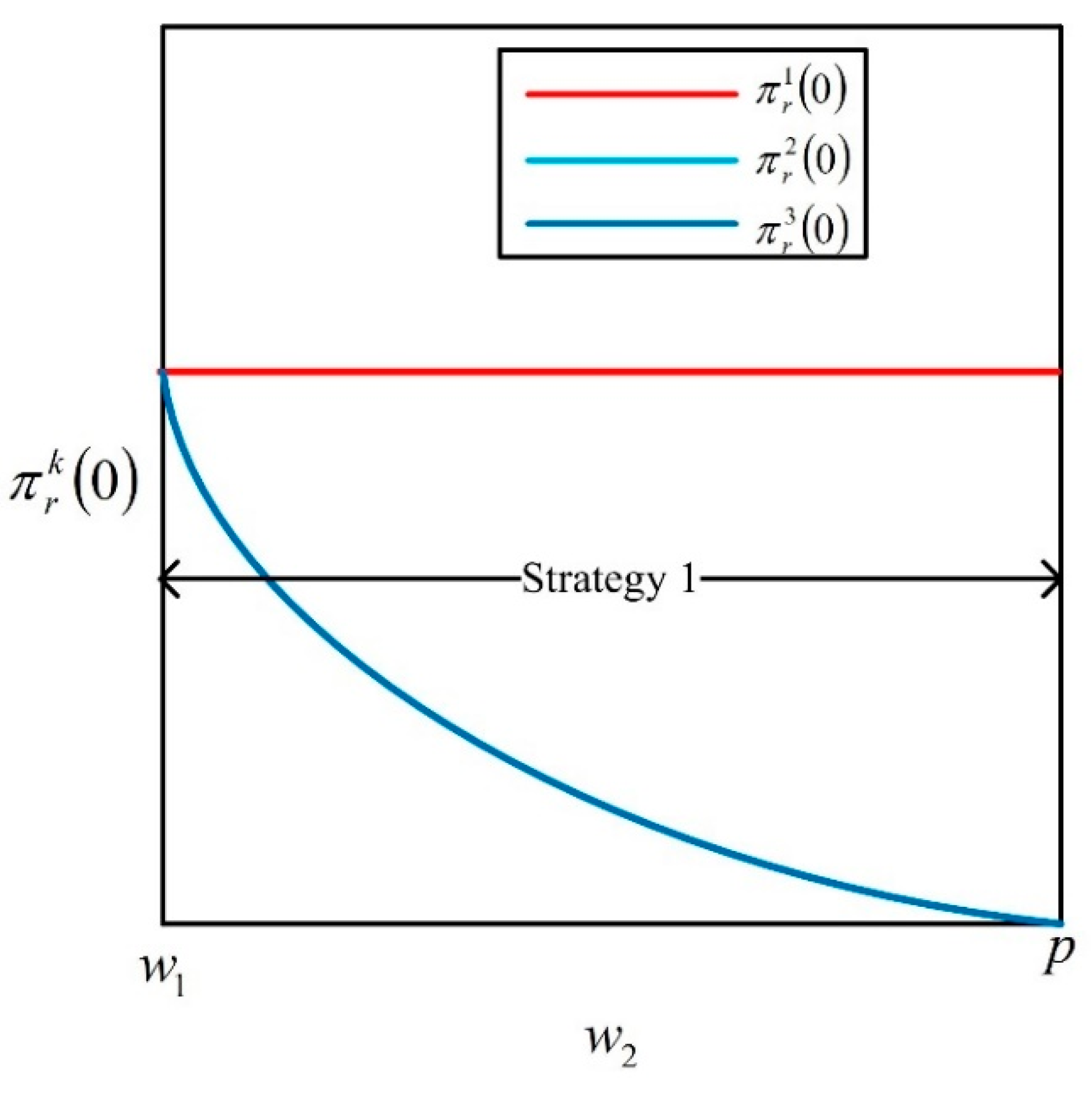
5. Strategy Selection

In this section, this paper studies the optimal production and order strategy for the supplier and the retailer, respectively. With different demand information update quality, the retailer and the supplier may have different selections. Without a loss of generality, this paper analyzes the value of demand information updates in two special cases: imperfect information with $\rho =0$ and perfect information with $\rho =1$. When $\rho \in \left(\mathrm{0,1}\right)$, it is challenging to obtain analytical results of the optimal strategy selection for the supplier and the retailer. Hence, this paper will conduct a numerical analysis in Section 6 to show the optimal strategy selection for the supplier and the retailer.

5.1. Imperfect Demand Signal with $\rho =0$

When $\rho =0$, the demand signal observed during the production does not have any impact on the demand uncertainty. Hence, the demand distribution at the beginning of the sales season satisfies $F\left(x|i\right)=F\left(x\right)$. When $\rho =0$ under strategy 1, the expected profit of the retailer is

$${\pi }_r^1\left(0\right)=\left(p-w_1\right)Q_0^1\left(0\right)-\left(p-v_r\right){\int }_0^{Q_0^1\left(0\right)}F\left(x\right)dx,$$

(21)

and the optimal order quantity of the retailer is $Q_0^1\left(0\right)=F^{-1}\left(\frac{p-w_1}{p-v_r}\right)$. Similarly, under strategy 2, the expected profit of the retailer is

$${\pi }_r^2\left(0\right)=\left(p-w_2\right)Q_1^2\left(0\right)-\left(p-v_r\right){\int }_0^{Q_1^2\left(0\right)}F\left(x\right)dx,$$

(22)

and the optimal order quantity of the retailer is $Q_1^2\left(0\right)=F^{-1}\left(\frac{p-w_2}{p-v_r}\right)$. Under strategy 3, the retailer’s expected profit and the order quantity are consistent with his counterpart under strategy 2, i.e., ${\pi }_r^2\left(0\right)={\pi }_r^3\left(0\right)$ and $Q_1^2\left(0\right)=Q_1^3\left(0\right)$. Since $w_1<w_2$, then $Q_0^1\left(0\right)>Q_1^2\left(0\right)=Q_1^3\left(0\right)$. Therefore, the retailer will always choose strategy 1 when the demand signal is imperfect (see schematic diagram, Figure 5).

Next, the strategy preference from the supplier’s perspective with $\rho =0$ is studied. Under strategy 1, adopting a “make-to-order” policy, the supplier’s optimal capacity quantity and regular production quantity equal the retailer’s optimal order quantity, i.e., $M_0^1\left(0\right)=M_1^1\left(0\right)=Q_0^1\left(0\right)$. Then, the expected profit of the supplier is

$${\pi }_s^1\left(0\right)=\left(w_1-c_0-c_1\right)Q_0^1\left(0\right).$$

(23)

The demand information is symmetric for both members. Thus, under strategy 2, the supplier would prepare capacity $M_0^2\left(0\right)=Q_1^2\left(0\right)$ and then produce $M_2^2\left(0\right)=Q_1^2\left(0\right)$ in the emergency mode. Then, the expected profit of the supplier is

$${\pi }_s^2\left(0\right)=\left(w_2-c_0-c_2\right)Q_1^2\left(0\right).$$

(24)

Similarly, under strategy 3, the supplier would prepare capacity $M_0^3\left(0\right)=Q^3\left(0\right)$ and then produce $M_1^3\left(0\right)=Q_1^3\left(0\right)$ in the regular mode. Then, the expected profit of the supplier is

$${\pi }_s^3\left(0\right)=\left(w_2-c_0-c_1\right)Q_1^3\left(0\right).$$

(25)

Since $c_2>c{}_1$ and $Q_1^2\left(0\right)=Q_1^3\left(0\right)$, then ${\pi }_s^2\left(0\right)<{\pi }_s^3\left(0\right)$. However, since $w_1<w_2$ and $Q_0^1\left(0\right)>Q_1^2\left(0\right)$, the relationship between ${\pi }_s^1\left(0\right)$ and ${\pi }_s^3\left(0\right)$ is not so clear.

Based on the above discussion, the optimal strategy selection for the supplier with imperfect information is as follows.

Proposition 5.

When $\rho =0$, there exist two threshold values $w_{21}\left(0\right)$ and $w_{22}\left(0\right)$ with $w_{22}\left(0\right)<w_{21}\left(0\right)$ such that:

(1) If $w_1\le w_2\le w_{22}\left(0\right)$, then ${\pi }_s^1\left(0\right)>{\pi }_s^3\left(0\right)>{\pi }_s^2\left(0\right)$, the supplier prefers strategy 1;

(2) If $w_{22}\left(0\right)\le w_2\le w_{21}\left(0\right)$, then ${\pi }_s^3\left(0\right)>{\pi }_s^1\left(0\right)>{\pi }_s^2\left(0\right)$, the supplier prefers strategy 3;

(3) If $w_{21}\left(0\right)\le w_2\le p$, then ${\pi }_s^3\left(0\right)>{\pi }_s^2\left(0\right)>{\pi }_s^1\left(0\right)$, the supplier prefers strategy 3;

where

$$w_{21}\left(0\right)=c_0+c_2+\left(w_1-c_0-c_1\right)\frac{Q_0^1\left(0\right)}{Q_1^2\left(0\right)},$$

(26)

$$w_{22}\left(0\right)=c_0+c_1+\left(w_1-c_0-c_1\right)\frac{Q_0^1\left(0\right)}{Q_1^2\left(0\right)}.$$

(27)

Proposition 5 shows that when the demand signal is imperfect, the supplier’s optimal strategy selection depends on $w_2$ (see schematic diagram Figure 6). If the retailer chooses to make a delay order, the supplier could charge a higher wholesale price (i.e., $w_2>w_1$), while the retailer would place a smaller order quantity (i.e., $Q_0^1\left(0\right)>Q_1^2\left(0\right)=Q_1^3\left(0\right)$). When $w_2$ is at a low level (i.e., $w_1\le w_2\le w_{22}\left(0\right)$), the supplier prefers the retailer to place order in advance. When $w_2$ is at a moderate level (i.e., $w_{22}\left(0\right)\le w_2\le w_{21}\left(0\right)$), the supplier prefers to achieve a larger profit from a delay order. For this case, either strategy 3 or strategy 2 is superior to strategy 1. It is worth noting that the supplier has the first-move advantage in strategy 3 compared with strategy 2. Without strategy 3, the supplier still prefers the retailer to make an advance order due to ${\pi }_s^1\left(0\right)>{\pi }_s^2\left(0\right)$. When $w_2$ is at a high level (i.e., $w_{21}\left(0\right)\le w_2\le p$), the supplier always prefers the retailer to make a delay order to obtain more profit. From Proposition 5, even though the demand information is not updated, the supplier still needs a trade-off between a higher wholesale price and a smaller order quantity from the retailer. This is consistent with the classical supply chain wholesale price contract theory.

Based on the above discussion, only when $w_1\le w_2\le w_{22}\left(0\right)$, there exists a strategy equilibrium in which both the supplier and the retailer prefer strategy 1 (see schematic diagram Figure 7). Otherwise, the retailer’s strategy preference is not consistent with the supplier’s strategy preference. Therefore, to induce the retailer to choose a strategy consistent to hers, the supplier could adjust the $w_2$ in the interval $\left[w_1,w_{22}\left(0\right)\right]$.

Theorem 1.

When $\rho =0$, if and only if $w_1\le w_2\le w_{22}\left(0\right)$, there exists a strategy equilibrium such that both the supplier and the retailer prefer strategy 1.

From Theorem 1, when the demand signal is imperfect, the retailer always prefers to make an advance order to avoid a larger wholesale price $w_2$. Although the supplier has an intention to make a delay order to obtain more profit when $w_{22}\left(0\right)\le w_2\le p$, it cannot be accepted by the retailer. Hence, in order to achieve supply chain cooperation, it is beneficial for the supplier to set $w_2$ in the interval $\left[w_1,w_{22}\left(0\right)\right]$. Then, in the case of $\rho =0$, the equilibrium strategy only can be strategy 1.

5.2. Perfect Demand Signal with $\rho =1$

When $\rho =1$, ${\mu }^{\prime }=\mu +\frac{\left(i-m\right)\sigma }{s}$ and ${\sigma }^{\prime }=0$. The demand during the sales season can be completely determined by the realized demand signal $i$, i.e., $x|i=\mu +\frac{\left(i-m\right)\sigma }{s}$. Hence, once the retailer observes $I=i$ at the beginning of the sales season, then he would order $\min \left\{\mu +\frac{\left(i-m\right)\sigma }{s}, M_0^k\left(1\right)\right\}$ with $k=1$, 2, 3. For this special case, the supply chain members’ optimal strategy selection is studied. First, the retailer’s optimal ordering strategy is analyzed. Under strategy 1, the expected profit of the retailer is

$$\begin{array}{ll}{\pi }_r^1\left(1\right)=\hfill & E_{\left\{x\right\}}\left[{p\min \left\{x,Q_0^1\left(1\right)\right\}+v_r\left(Q_0^1\left(1\right)-x\right)}^{+}-w_1{Q}_0^1\left(1\right)\right]\\ & =\left(p-w_1\right)Q_0^1\left(1\right)-\left(p-v_r\right){\int }_0^{Q_0^1\left(1\right)}F\left(x\right)dx,\end{array}$$

(28)

and the optimal ordering quantity of the retailer is $Q_0^1\left(1\right)=F^{-1}\left(\frac{p-w_1}{p-v_r}\right)$.

Similarly, under strategy 2, the expected profit of the retailer is

$$\begin{array}{c}{\pi }_r^2\left(1\right)=E_{\left\{i\right\}}\left[\left(p-w_2\right)\min \left\{\mu +\frac{\left(i-m\right)\sigma }{s}, M_0^2\left(1\right)\right\}\right]\\ =\left(p-w_2\right)\left[{\int }_0^{i_{M_0^2\left(1\right)}}\left[\mu +\frac{\left(i-m\right)\sigma }{s}\right]dG\left(i\right)+{\int }_{i_{M_0^2\left(1\right)}}^{+\infty }{M}_0^2\left(1\right)dG\left(i\right)\right],\end{array}$$

(29)

where $i_{M_0^2\left(1\right)}=m+\frac{\left(M_0^2\left(1\right)-\mu \right)s}{\sigma }$, and $M_0^2\left(1\right)$ is the supplier’s capacity quantity under strategy 2. The retailer’s optimal ordering quantity is $Q_1^2\left(1\right)=\min \left\{\mu +\frac{\left(i-m\right)\sigma }{s}, M_0^2\left(1\right)\right\}$.

Under strategy 3, from Propositions 3 and 4, $M_0^2\left(1\right)=M_0^3\left(1\right)$. Then, $Q_1^2\left(1\right)=Q_1^3\left(1\right)=\min \left\{\mu +\frac{\left(i-m\right)\sigma }{s}, M_0^2\left(1\right)\right\}$. Hence, the retailer’s expected profit is consistent with his counterpart under strategy 2, i.e., ${\pi }_r^2\left(1\right)={\pi }_r^3\left(1\right)$. The following proposition shows the optimal strategy selection of the retailer when the demand signal is perfect.

Proposition 6.

When $\rho =1$, then there exists a threshold value $w_{21}\left(1\right)$ such that:

(1) If $w_1\le w_2\le w_{21}\left(1\right)$, then ${\pi }_r^1\left(1\right)\le {\pi }_r^2\left(1\right)={\pi }_r^3\left(1\right)$, the retailer prefers strategy 2 or 3;

(2) If $w_{21}\left(1\right)\le w_2\le p$, then ${\pi }_r^1\left(1\right)\ge {\pi }_r^2\left(1\right)={\pi }_r^3\left(1\right)$, the retailer prefers strategy 1; where

$$w_{21}\left(1\right)=p-\frac{E_{\left\{x\right\}}\left[{p\min \left\{x,Q_0^1\left(1\right)\right\}+v_r\left(Q_0^1\left(1\right)-x\right)}^{+}-w_1{Q}_0^1\left(1\right)\right]}{E_{\left\{i\right\}}\left[\min \left\{\mu +\frac{\left(i-m\right)\sigma }{s}, M_0^2\left(1\right)\right\}\right]}.$$

(30)

Proposition 6 shows that even though the demand signal is perfect, the retailer’s optimal strategy selection still depends on $w_2$ (see schematic diagram Figure 8). When the retailer places an order at $t=t_1$, he would have more accurate demand information (i.e., $var\left(x|i\right)<var\left(x\right)$), while he also would be charged a higher wholesale price (i.e., $w_2>w_1$). The retailer has to evaluate the trade-off between more accurate demand information and a higher wholesale price at $t=t_1$. From Proposition 6, only when $w_2$ is at a low level (i.e., $w_1\le w_2\le w_{21}\left(1\right)$), the retailer would obtain more profit under strategy 2 or 3 compared with strategy 1. However, when $w_2$ is at a high level (i.e., $w_{21}\left(1\right)\le w_2\le p$), it is costly for the retailer to make a delay order.

Next, the strategy selection from the supplier’s perspective with $\rho =1$ is studied. Under strategy 1, by “make-to-order” policy, $M_0^1\left(1\right)=M_1^1\left(1\right)=Q_0^1\left(1\right)$ and the expected profit of the supplier is

$${\pi }_s^1\left(1\right)=\left(w_1-c_0-c_1\right)Q_0^1\left(1\right).$$

(31)

Under strategy 2, the supplier needs to prepare capacity $M_0^2\left(1\right)$ in advance at $t=t_0$. Then, by adopting a “make-to-order” policy, she would produce $M_2^2\left(1\right)=Q_1^2\left(1\right)=\min \left\{\mu +\frac{\left(i-m\right)\sigma }{s}, M_0^2\left(1\right)\right\}$ in the emergency mode at $t=t_1$. For this case, the expected profit of the supplier is

$$\begin{array}{c}{\pi }_s^2\left(1\right)=-c_0{M}_0^2\left(1\right)+E_{\left\{i\right\}}\left[\left(w_2-c_2\right)Q_1^2\left(1\right)+v_0{\left(M_0^2\left(1\right)-Q_1^2\left(1\right)\right)}^{+}\right]\\ =\left(w_2-c_2-c_0\right)M_0^2\left(1\right)-\left(w_2-c_2-v_0\right)\left[{\int }_0^{i_{M_0^2\left(1\right)}}\left(M_0^2\left(1\right)-\mu -\frac{\left(i-m\right)\sigma }{s}\right)dG\left(i\right)\right].\end{array}$$

(32)

Under strategy 3, the supplier prepares capacity $M_0^3\left(1\right)$ and produces $M_1^3\left(1\right)$ at $t=t_0$ in the regular mode. Then, the supplier produces ${\left[\min \left\{M_0^3\left(1\right), Q_1^3\left(1\right)\right\}-M_1^3\left(1\right)\right]}^{+}$ at $t=t_1$ in the emergency mode. In this case, the expected profit of the supplier is

$$\begin{array}{l}\hspace{1em}{\pi }_s^3\left(1\right)\\ =-c_0{M}_0^3\left(1\right)-c_1{M}_1^3\left(1\right)+E_{\left\{i\right\}}[w_2{Q}_1^3\left(1\right)-c_2{\left[\min \left\{M_0^3\left(1\right),Q_1^3\left(1\right)\right\}-M_1^3\left(1\right)\right]}^{+}+v_0[M_0^3\left(1\right)-\\ {\max \left\{M_1^3\left(1\right),Q_1^3\left(1\right)\right\}]}^{+}+v_s{\left(M_1^3\left(1\right)-Q_1^3\left(1\right)\right)}^{+}]\hfill \\ =\left(w_2-c_2-c_0\right)M_0^3\left(1\right)-\left(w_2-c_2-v_0\right){\int }_0^{i_{M_0^3\left(1\right)}}\left(M_0^3\left(1\right)-\mu -\frac{\left(i-m\right)\sigma }{s}\right)dG\left(i\right)+\left(c_2-c_1\right)M_1^3\left(1\right)-\hfill \\ \left(c_2+v_0-v_s\right){\int }_0^{i_{M_1^3\left(1\right)}}\left(M_1^3\left(1\right)-\mu -\frac{\left(i-m\right)\sigma }{s}\right)dG\left(i\right),\end{array}$$

(33)

where $i_{M_0^3\left(1\right)}=m+\frac{\left(M_0^3\left(1\right)-\mu \right)s}{\sigma }$ and $i_{M_1^3\left(1\right)}=m+\frac{\left(M_1^3\left(1\right)-\mu \right)s}{\sigma }$.

Note that, $M_0^2\left(1\right)=M_0^3\left(1\right)$ and $Q_1^2\left(1\right)=Q_1^3\left(1\right)$. Thus,

$$\begin{array}{l}{\pi }_s^2\left(1\right)-{\pi }_s^3\left(1\right)\\ =-\left(c_2-c_1\right)M_1^3\left(1\right)+\left(c_2+v_0-v_s\right){\int }_0^{i_{M_1^3\left(1\right)}}\left(M_1^3\left(1\right)-\mu -\frac{\left(i-m\right)\sigma }{s}\right)dG\left(i\right),\end{array}$$

(34)

Because of $c_2>c_1>v_s$, neither strategy 2 nor strategy 3 is the dominant strategy when the realized demand signal is perfect. Differently from the case of $\rho =0$, in this case, the supplier not only needs to make a trade-off between a higher wholesale price and a lower ordering quantity, but also has to make a trade-off between a higher wholesale price and a higher production cost, which leads to the following proposition.

Proposition 7.

When $\rho =1$, there exist three threshold values $c_2\left(1\right)$, $w_{22}\left(1\right)$ and $w_{23}\left(1\right)$ such that:

(1) When $c_1<c_2\le c_2\left(1\right)$, then ${\pi }_s^2\left(1\right)\ge {\pi }_s^3\left(1\right)$, $w_{23}\left(1\right)\ge w_{22}\left(1\right)$ and: If $w_1\le w_2\le w_{22}\left(1\right)$, then ${\pi }_s^1\left(1\right)\ge {\pi }_s^2\left(1\right)\ge {\pi }_s^3\left(1\right)$, and thus, the supplier prefers strategy 1; If $w_{22}\left(1\right)\le w_2\le p$, ${\pi }_s^2\left(1\right)\ge {\pi }_s^1\left(1\right), {\pi }_s^2\left(1\right)\ge {\pi }_s^3\left(1\right)$, thus, the supplier prefers strategy 2.

(2) When $c_2\left(1\right)\le c_2<w_1$, then ${\pi }_s^2\left(1\right)\le {\pi }_s^3\left(1\right)$, $w_{23}\left(1\right)\le w_{22}\left(1\right)$ and: If $w_1\le w_2\le w_{22}\left(1\right)$, then ${\pi }_s^1\left(1\right)\ge {\pi }_s^3\left(1\right)\ge {\pi }_s^2\left(1\right)$, and thus, the supplier prefers strategy 1; If $(w_{22}\left(1\right)\le w_2\le p$, ${\pi }_s^3\left(1\right)\ge {\pi }_s^1\left(1\right), {\pi }_s^3\left(1\right)\ge {\pi }_s^2\left(1\right)$, and thus, the supplier prefers strategy 3;

where

$$c_2\left(1\right)=\frac{c_1{M}_1^3\left(1\right)+\left(v_0-v_s\right){\int }_0^{i_{M_1^3\left(1\right)}}\left(M_1^3\left(1\right)-\mu -\frac{\left(i-m\right)\sigma }{s}\right)dG\left(i\right)}{M_1^3\left(1\right)-{\int }_0^{i_{M_1^3\left(1\right)}}\left(M_1^3\left(1\right)-\mu -\frac{\left(i-m\right)\sigma }{s}\right)dG\left(i\right)},$$

(35)

$$w_{22}\left(1\right)=\frac{\left(c_2+c_0\right)M_0^2\left(1\right)-\left(c_2+v_0\right){\int }_0^{i_{M_0^2\left(1\right)}}\left(M_0^2\left(1\right)-\mu -\frac{\left(i-m\right)\sigma }{s}\right)dG\left(i\right)+\left(w_1-c_0-c_1\right)Q_0^1\left(1\right)}{M_0^2\left(1\right)-{\int }_0^{i_{M_0^2\left(1\right)}}\left(M_0^2\left(1\right)-\mu -\frac{\left(i-m\right)\sigma }{s}\right)dG\left(i\right)},$$

(36)

$$w_{23}\left(1\right)=w_{21}\left(1\right)+\frac{ {\pi }_s^2\left(1\right)-{\pi }_s^3\left(1\right)}{M_0^3\left(1\right)-{\int }_0^{i_{M_0^3\left(1\right)}}\left(M_0^3\left(1\right)-\mu -\frac{\left(i-m\right)\sigma }{s}\right)dG\left(i\right)}.$$

(37)

From Proposition 7, when the demand signal is perfect, the supplier’s optimal strategy selection depends on both the wholesale price in a delay order (i.e., $w_2$) and the production cost in the emergency mode (i.e., $c_2$). There exist two trade-offs that affect the supplier’s strategy selection. First, comparing strategies 2 and 3, the supplier’s optimal strategy selection depends on $c_2$. The supplier faces a higher average production cost in strategy 2 while takes a greater risk of overproduction and overcapacity in strategy 3. Hence, the supplier has to make a trade-off between a higher average production cost and a bigger overproduction risk between strategies 2 and 3. Second, comparing strategies 1, and 2 or 3, the supplier’s optimal strategy selection depends on $w_2$. Because of the trade-off between a higher wholesale price and a larger overproduction risk in strategy 2 or 3, the supplier does not always choose one strategy over the other. To be more specific, when $c_2$ is at a low level (i.e., $c_1<c_2\le c_2\left(1\right)$), it is beneficial for the supplier to choose strategy 2 rather than strategy 3 to avoid overproduction risk (see schematic diagram Figure 9(1)). Then, when $w_2$ is at a low level (i.e., $w_1\le w_2\le w_{22}\left(1\right)$), the supplier would choose strategy 1 without overproduction risk. When $w_2$ is at a high level (i.e., $w_{22}\left(1\right)\le w_2\le p$), the supplier prefers strategy 2 to obtain more profit. A similar discussion is shown in schematic diagram Figure 9(2).

Finally, the strategy equilibrium of production and ordering with $\rho =1$ is analyzed. Let

$$p\left(1\right)=\frac{\begin{array}{c}\left(c_2+c_0\right)M_0^2\left(1\right)-\left(c_2+v_0\right){\int }_0^{i_{M_0^2\left(1\right)}}\left(M_0^2\left(1\right)-\mu -\frac{\left(i-m\right)\sigma }{s}\right)dG\left(i\right)\\ +\left(w_1-c_0-c_1\right)Q_0^1\left(1\right)+{\pi }_r^1\left(1\right)\end{array}}{M_0^2\left(1\right)-{\int }_0^{i_{M_0^2\left(1\right)}}\left(M_0^2\left(1\right)-\mu -\frac{\left(i-m\right)\sigma }{s}\right)dG\left(i\right)},$$

(38)

then $w_{22}\left(1\right)-w_{21}\left(1\right)=p\left(1\right)-p$ and

$$w_{23}\left(1\right)-w_{21}\left(1\right)=\frac{ {\pi }_s^2\left(1\right)-{\pi }_s^3\left(1\right)}{M_0^3\left(1\right)-{\int }_0^{i_{M_0^3\left(1\right)}}\left(M_0^3\left(1\right)-\mu -\frac{\left(i-m\right)\sigma }{s}\right)dG\left(i\right)}.$$

(39)

According to Proposition 7(1), when $c_1<c_2\le c_2\left(1\right)$, then $w_{23}\left(1\right)\ge w_{22}\left(1\right)$ and ${\pi }_s^2\left(1\right)-{\pi }_s^3\left(1\right)\ge 0$. Hence, $w_{23}\left(1\right)\ge w_{21}\left(1\right)$. If $p\left(1\right)\ge p$, then $w_{22}\left(1\right)\ge w_{21}\left(1\right)$. Therefore, $w_{23}\left(1\right)\ge w_{22}\left(1\right)\ge w_{21}\left(1\right)$. In this case, only when $w_{21}\left(1\right)\le w_2\le w_{22}\left(1\right)$, the strategy equilibrium exists in which both members prefer strategy 1 (see schematic diagram Figure 10(1)). If $p\left(1\right)\le p$, then $w_{22}\left(1\right)\le w_{21}\left(1\right)$. Therefore, $w_{23}\left(1\right)\ge w_{21}\left(1\right)\ge w_{22}\left(1\right)$. In this case, only when $w_{22}\left(1\right)\le w_2\le w_{21}\left(1\right)$, the strategy equilibrium exists in which both members prefer strategy 2 (see schematic diagram Figure 10(2)). According to Proposition 7(2), when $c_2\left(1\right)\le c_2<w_1$, then $w_{23}\left(1\right)\le w_{22}\left(1\right)$ and ${\pi }_s^2\left(1\right)-{\pi }_s^3\left(1\right)\le 0$. Hence, $w_{23}\left(1\right)\le w_{21}\left(1\right)$. Similarly, if $p\left(1\right)\ge p$, then $w_{22}\left(1\right)\ge w_{21}\left(1\right)$ and $w_{22}\left(1\right)\ge w_{21}\left(1\right)\ge w_{23}\left(1\right)$. Therefore, only when $w_{21}\left(1\right)\le w_2\le w_{22}\left(1\right)$, the strategy equilibrium exists in which both members prefer strategy 1 (see schematic diagram Figure 10(3)). If $p\left(1\right)\le p$, then $w_{22}\left(1\right)\le w_{21}\left(1\right)$ and $w_{21}\left(1\right)\ge w_{22}\left(1\right)\ge w_{23}\left(1\right)$. Therefore, only when $w_{22}\left(1\right)\le w_2\le w_{21}\left(1\right)$, the strategy equilibrium exists in which both members prefer strategy 3 (see schematic diagram Figure 10(4)).

Theorem 2.

When $\rho =1$, then

(1) When $p\left(1\right)\ge p$, if and only if $w_{21}\left(1\right)\le w_2\le w_{22}\left(1\right)$, there exists a strategy equilibrium such that both the supplier and the retailer prefer strategy 1;

(2) When $p\left(1\right)\le p$ and $c_1<c_2\le c_2\left(1\right)$, if and only if $w_{22}\left(1\right)\le w_2\le w_{21}\left(1\right)$, there exists a strategy equilibrium such that both the supplier and the retailer prefer strategy 2;

(3) If $p\left(1\right)\le p$ and $c_2\left(1\right)\le c_2<w_1$, if and only if $w_{22}\left(1\right)\le w_2\le w_{21}\left(1\right)$, there exists a strategy equilibrium such that both the supplier and the retailer prefer strategy 3.

Unlike Theorem 1 with $\rho =0$, when $\rho =1$, Theorem 2 shows that all three strategies discussed in this paper are likely to be the equilibrium strategy under certain conditions. The equilibrium strategy is influenced by the wholesale price in a delay order (i.e., $w_2$), the production cost in the emergency mode (i.e., $c_2$) and the retail price (i.e., $p$). In most business practices, the wholesale price is determined by the supplier. Therefore, to manipulate the retailer to choose a strategy consistent with hers, the supplier can adjust the wholesale price to achieve supply chain cooperation and profit-maximizing.

6. Numerical Simulation

In this section, the equilibrium of production and ordering strategy with a general demand information update quality (i.e., $0<\rho <1$) is studied through numerical simulation. Similarly to [28,30], the relevant parameters settings for demand obeying a normal distribution are as follows: $\mu =$ 200, $\sigma =$ 60, $m=$ 100, $s=$ 30; referring to [33,37], some other parameters can be set as follows: $c_0=$ 20, $c_1=$ 40, $c_2=$ 45, $v_0=$ 18, $v_s=$ 35, $v_r=$ 30, $w_1=$ 65, $w_2=$ 85, $p=$ 100, $\rho =\sqrt{3}$/2. To facilitate the analysis, when a parameter is analyzed, the values of the other parameters remain at the initial setting as shown above.

First, this section analyzes how the wholesale prices $w_2$ affects the profits and strategy selection of supply chain members. Without loss of generality, assume that the wholesale price in advance orders is fixed (i.e., $w_1=65$), and only the wholesale price in a delay order is variable, which ranges from 66 to 99 (i.e., $65\le w_2\le 99$). Given $\rho =\sqrt{3}$/2, Figure 11 shows the profits of supply chain members with three strategies. From Figure 11, the profits of the retailer and the supplier under strategy 1 are fixed (i.e., ${\pi }_r^1=5330.92$, ${\pi }_s^1=1000$). However, under strategies 2 and 3, the retailer’s profit decreases in $w_2$. There exists a threshold value $w_r^1=68.36$ such that ${\pi }_r^1={\pi }_r^2={\pi }_r^3$. When $65\le w_2\le 68.36$, then ${\pi }_r^1\le {\pi }_r^2={\pi }_r^3$, and the retailer chooses strategies 2 and 3. When $68.36\le w_2\le 100$, then ${\pi }_r^1\ge {\pi }_r^2={\pi }_r^3$, and the retailer chooses strategy 1. For the supplier, her profit is concave with respect to $w_2$ under strategies 2 and 3. To be more specific, there will exist two threshold values $w_s^1=67.48$ and $w_s^2=70.85$ such that ${\pi }_s^1={\pi }_s^3$ and ${\pi }_s^2={\pi }_s^3$, respectively. When $65\le w_2\le 67.48$, then ${\pi }_s^1\ge {\pi }_s^3\ge {\pi }_s^2$ and the supplier prefers strategy 1. When $67.46\le w_2\le 70.85$ and $70.85\le w_2\le 99$, then ${\pi }_s^3\ge {\pi }_s^1\ge {\pi }_s^2$ and ${\pi }_s^3\ge {\pi }_s^2\ge {\pi }_s^1$, and the supplier prefers strategy 3. Therefore, there exists an equilibrium region $67.48\le w_2\le 68.36$, in which both the retailer and the supplier prefer strategy 3. This is consistent with Theorem 2(3).

The range of $w_2$ is divided into four cases through the threshold values $w_s^1$, $w_r^1$ and $w_s^2$. Next, for a given $w_2$, the profits of the supply chain members with respect to the quality of demand information updates (i.e., $\rho$) are analyzed under different cases. The $\rho$ varies from 0.1 to 0.9. Specifically, Figure 12(1) presents the supply chain members’ profits when $w_1<w_2=66<w_s^1$. Similarly, Figure 12(2)–(4) present the cases of $w_s^1<w_2=68<w_r^1$, $w_r^1<w_2=70<w_s^2$ and $w_s^2<w_2=72<p$, respectively. In the above four cases, under strategy 1, the supply chain members’ profits are fixed as $\rho$ increases. This is reasonable since under strategy 1, neither the supplier nor the retailer can take advantage of demand information updates under strategy 1. Under strategies 2 and 3, the retailer’s profit always increases in $\rho$, while the supplier’s profit keeps decreasing in $\rho$. This is because when the retailer adopts delay orders, he could take advantage of demand information updates. As $\rho$ increases, the accuracy of the demand forecast is higher and the mismatch between the retailer’s order and the market demand is smaller. As a result, the retailer’s profit increases. However, due to a long production season, the supplier needs to prepare capacity in advance. Once the retailer makes a delay order after demand information updates, the mismatch between the supplier’s production and the retailer’s order increases as $\rho$ increases. Hence, the supplier’s profit decreases.

Furthermore, for the retailer, he must make a trade-off between a high wholesale price (i.e., $w_2$) and more accurate demand information (i.e., $\rho$) at $t=t_2$; Similarly, for the supplier, she has to make a trade-off between a high revenue from the retailer (i.e., $w_2$) and a large overproduction risk (i.e., $\rho$) at $t=t_2$. Hence, there are some differences between the retailer’s and supplier’s strategy selection as follows. As can be seen from Figure 12(1), since $w_2-w_1$ is small, the retailer always benefits more from demand information updates (i.e., ${\pi }_r^2={\pi }_r^3>{\pi }_r^1$). Hence, the retailer prefers strategies 2 and 3 when $w_1<w_2=66<w_s^1$. However, there exists a ${\rho }_1=$ 0.36 such that ${\pi }_s^1={\pi }_s^3>{\pi }_s^1$. When $0<\rho <{\rho }_1=$ 0.36, the supplier could benefit from demand information updates with a high revenue from the retailer (i.e., ${\pi }_s^3>{\pi }_s^1>{\pi }_s^2$). Then, the supplier prefers strategy 3. When ${\rho }_1<\rho <1$, the supplier cannot benefit from demand information updates with a great overproduction risk (i.e., ${\pi }_s^1>{\pi }_s^3>{\pi }_s^2$). Then, the supplier prefers strategy 1. This is consistent with [22]. And there exists an equilibrium region $\left(w_2,\rho \right)=\left(w_1,w_s^1\right)\times \left(0,{\rho }_1\right)$ in which both the retailer and the supplier prefer strategy 3. From Figure 12(2), when $w_2$ increases to $w_s^1<w_2=68<w_r^1$, both the retailer and the supplier could benefit from demand information updates. Therefore, there exists an equilibrium area $\left(w_2,\rho \right)=\left(w_s^1,w_r^1\right)\times \left(\mathrm{0,1}\right)$ in which both the retailer and the supplier prefer strategy 3. However, when $w_2$ increases to $w_r^1<w_2=70<w_s^2$ and $w_s^2<w_2=72<p$, since $w_2-w_1$ is big, only the supplier can benefit from demand information updates. Hence, there does not exist any equilibrium area.

Finally, according to the discussion in Figure 12, for a given demand information update quality, it can be concluded that the equilibrium of production and ordering strategy mainly depends on the wholesale price in delay orders. In addition, it can be seen from Figure 12 that, for a given $w_2$, the equilibrium of production and ordering strategy also depends on the quality of demand information updates. The strategic selection of both suppliers and retailers will be affected by $w_2$ and $\rho$. Therefore, Figure 13 draws an equilibrium graph of production and ordering strategy for the supplier and the retailer. The optimal strategy selection of supply chain members is divided into three regions. In region I, both the retailer and the supplier prefer strategy 3, which is also a unique equilibrium. However, in regions II and III, the retailer and the supplier have different preferences. Thus, there does not exist a strategy equilibrium. The final strategy selection depends on individual supply chain members’ negotiating powers. If the retailer’s negotiating power is higher, in regions II and III, strategy 1 would be adopted by the supply chain even if it is non-equilibrium. Otherwise, the final strategy chosen by the supply chain is strategy 3.

7. Conclusions and Management Insights

7.1. Conclusions and Theoretical Contribution

This paper investigates the management problems of production and order in a two-echelon supply chain with demand information updates and capacity restrictions. Due to a long production lead time, the supplier needs to prepare capacity in advance. The demand information is updated during the supplier’s production season. The retailer can order before or after demand information updates, which is denoted as an advance order or delay order. If the retailer chooses to make an advance order, the supplier adopts the regular mode; if the retailer chooses to make a delay order, the supplier adopts the emergency mode or a two-mode production system. Under the above settings, this paper studies the supplier’s optimal production strategy and the retailer’s optimal order strategy in three Stackelberg game models. By comparing the expected profits of supply chain members under three production and ordering strategies, this paper further explores the strategy preference of supply chain members and obtains a strategy equilibrium under certain conditions. The research shows that the strategy preference of supply chain members is affected by the wholesale price under a delay order, the emergency production cost, and the quality of demand information updates.

Specifically, the theoretical results show the following: (1) If updated demand information is imperfect, the strategy preference of supply chain members is only related to the wholesale price under a delay order. Only when the wholesale price under a delay order is at a low level, strategy 1 is a unique strategy equilibrium which is preferred by both the supplier and the retailer. (2) If updated demand information is perfect, the strategy preference of supply chain members is related not only to the wholesale price under a delay order but also to the emergency production costs. When the retail price is at a high level, only when the wholesale price under a delay order is at middle level, strategy 1 is a unique strategy equilibrium. When the retail price is at a low level, only when the emergency production cost is at a low level, strategy 2 is a unique strategy equilibrium; otherwise, strategy 3 is a unique strategy equilibrium. (3) If updated demand information is general, the strategy preference of supply chain members is related by both the wholesale price under a delay order and the quality of demand information updates. Only when both the wholesale price under a delay order and the quality of demand information updates are at a low level or the wholesale price under a delay order is at a middle level, strategy 3 is a unique strategy equilibrium.

7.2. Management Insights and Practical Application

Our work points out two important managerial insights. First, when the wholesale price under a delay order is at a high level, he should choose to make an advance order to reduce the order cost; otherwise, he should choose delay orders to reduce the order risk. Second, the supplier who needs to produce in advance could set the appropriate wholesale price under a delay order to induce the retailer to choose an order strategy consistent with hers. For example, if the supplier prefers strategy 2 or 3, she should set a smaller wholesale price under a delay order to induce the retailer to choose delay orders. On the contrary, if the supplier prefers strategy 1, a larger wholesale price should be set under delayed orders to induce the retailer to choose to make advance orders.

The practical application of this paper is reflected in the following three aspects: First, it elaborates the actual value of demand information update to the retailer. When the wholesale price after demand information update is too high, the retailer will choose to order before the demand information is updated even though demand information update is perfect. It suggests that the value of demand information update is limited. Hence, retail enterprises need to consider the potential operating costs of demand information updates when attempting to update demand information. Second, the supplier with a long production lead time can offset the losses caused by demand information updates by increasing wholesale prices after demand information is updated, thereby reducing the retailer’s gains. Third, demand information update can reduce demand uncertainty, which is of great significance for improving the overall benefits of the supply chain. However, the separation of production and order decisions under demand information updates exacerbates the double marginal effect of the supply chain. Therefore, it is necessary for supply chain members to negotiate wholesale prices to reduce decision conflicts in an environment where demand information is updated.

7.3. Future Research

The paper can be extended in the following two possible directions. First, this study assumes that the supplier’s wholesale price after demand information updates is exogenous. The previous discussion shows that the supplier can adjust the wholesale price after demand information updates to reduce losses and capture the retailer’s gain. Hence, determining how to utilize updated demand information to set appropriate wholesale prices after demand information updates become a crucial challenge for the supplier. Second, the current model of this research only studies production and ordering strategies with the wholesale price contract. In fact, flexible contracts, such as options contracts, are increasingly used in supply chain management due to higher demand risks. As a natural extension of our work, future studies could consider the role of options in the supply chain coordination with demand information updates.

References

1. Chew, E.P.; Lee, L.H.; Sim, C.K. The impact of supply chain visibility when lead time is random. OR Spectr. 2013, 35, 163–190. [Google Scholar] [CrossRef]
2. Voigt, G.; Inderfurth, K. Supply chain coordination and setup cost reduction in case of asymmetric information. OR Spectr. 2011, 33, 99–122. [Google Scholar] [CrossRef]
3. Zhai, Y.Z.; Xue, W.L.; Ma, L.J. Commitment decisions with demand information updates and a capital-constrained supplier. Int. Trans. Oper. Res. 2020, 27, 2294–2316. [Google Scholar] [CrossRef]
4. Jin, M.; Wu, S.D. Capacity reservation contracts for high-tech industry. Eur. J. Oper. Res. 2007, 176, 1659–1677. [Google Scholar] [CrossRef]
5. Shen, B.; Choi, T.M.; Minner, S. A review on supply chain contracting with information considerations: Information updating and information asymmetry. Int. J. Prod. Res. 2019, 57, 4898–4936. [Google Scholar] [CrossRef]
6. Guo, L. The benefits of downstream information acquisition. Mark. Sci. 2009, 28, 457–471. [Google Scholar] [CrossRef]
7. Zhao, Y.X.; Wang, S.Y.; Cheng, T.C.E.; Yang, X.Q.; Huang, Z.M. Coordination of supply chains by option contracts: A cooperative game theory approach. Eur. J. Oper. Res. 2010, 207, 668–675. [Google Scholar] [CrossRef]
8. Yang, D.Q.; Xiao, T.J.; Choi, T.M.; Cheng, T.C.E. Optimal reservation pricing strategy for a fashion supply chain with forecast update and asymmetric cost information. Int. J. Prod. Res. 2018, 56, 1960–1981. [Google Scholar] [CrossRef]
9. Zheng, M.M.; Shunko, M.; Gavirneni, N.; Shu, Y.; Wu, K. Reactive production with capacity restriction in supply chains with forecast updates. IISE Trans. 2019, 51, 142–1436. [Google Scholar] [CrossRef]
10. Barnes-Schuster, D.; Bassok, Y.; Anupindi, R. Coordination and flexibility in supply contracts with options. Manuf. Serv. Oper. Manag. 2002, 4, 171–207. [Google Scholar] [CrossRef]
11. Li, J.C.; Zhou, Y.W.; Huang, W.Y. Production and procurement strategies for seasonal product supply chain under yield uncertainty with commitment-option contracts. Int. J. Prod. Econ. 2017, 183, 208–222. [Google Scholar] [CrossRef]
12. Xu, H. Managing production and procurement through option contracts in supply chains with random yield. Int. J. Prod. Econ. 2010, 126, 306–313. [Google Scholar] [CrossRef]
13. Wu, M.C.; Ma, L.J.; Xue, W.L. Order timing for manufacturers with spot purchasing price uncertainty and demand information updates. J. Syst. Sci. Syst. Eng. 2020, 29, 631–654. [Google Scholar] [CrossRef]
14. Zhou, Y.W.; Wang, S.D. Supply chain coordination for newsvendor-type products with two ordering opportunities and demand information update. J. Oper. Res. Soc. 2012, 63, 1655–1678. [Google Scholar] [CrossRef]
15. Donohue, K.L. Efficient supply contracts for fashion goods with forecast updating and two production modes. Manag. Sci. 2000, 46, 1397–1411. [Google Scholar] [CrossRef]
16. Zhou, Y.W.; Wang, S.D. Manufacturer-buyer coordination for newsvendor-type-products with two ordering opportunities and partial backorders. Eur. J. Oper. Res. 2009, 198, 958–974. [Google Scholar] [CrossRef]
17. Choi, T.M.; Li, D.; Yan, H.M. Quick response policy with Bayesian information updates. Eur. J. Oper. Res. 2006, 170, 788–808. [Google Scholar] [CrossRef]
18. Cachon, G.P.; Swinney, R. Purchasing, pricing and quick response in the presence of strategic consumers. Manag. Sci. 2009, 55, 497–511. [Google Scholar] [CrossRef]
19. Cachon, G.P.; Swinney, R. The value of fast fashion: Quick response, enhanced design, and strategic consumer behavior. Manag. Sci. 2011, 57, 778–795. [Google Scholar] [CrossRef]
20. Li, T.Y.; Fang, W.G.; Baykal-Gursoy, M. Two-stage inventory management with financing under demand updates. Int. J. Prod. Econ. 2021, 232, 107915. [Google Scholar] [CrossRef]
21. Shi, Y.; Guo, X.L.; Yu, Y.G. Dynamic warehouse size, planning with demand forecast and contract flexibility. Int. J. Prod. Res. 2018, 56, 1313–1325. [Google Scholar] [CrossRef]
22. Wu, J.H. Quantity flexibility contracts under Bayesian updating. Comput. Oper. Res. 2005, 32, 1267–1288. [Google Scholar] [CrossRef]
23. Wang, Q.Z.; Tsao, D.B. Supply contract with bidirectional options: The buyer’s perspective. Int. J. Prod. Econ. 2006, 101, 30–52. [Google Scholar] [CrossRef]
24. Zheng, M.M.; Wu, K.; Shu, Y. Newsvendor problems with demand forecast updating and supply constraints. Comput. Oper. Res. 2016, 67, 193–206. [Google Scholar] [CrossRef]
25. Choi, T.M.; Li, D.; Yan, H. Optimal two-stage ordering policy with Bayesian information updating. J. Oper. Res. Soc. 2003, 54, 846–859. [Google Scholar] [CrossRef]
26. Choi, T.M. Incorporating social media observations and bounded CrossMark rationality into fashion quick response supply chains in the big data era. Transp. Res. Part E-Logist. Transp. Rev. 2018, 114, 386–397. [Google Scholar] [CrossRef]
27. Choi, T.M. Internet based elastic logistics platforms for fashion quick response systems in the digital era. Transp. Res. Part E-Logist. Transp. Rev. 2020, 143, 102096. [Google Scholar] [CrossRef]
28. Chen, H.Y.; Chen, J.; Chen, Y.H. A coordination mechanism for a supply chain with demand information updates. Int. J. Prod. Econ. 2006, 103, 347–361. [Google Scholar] [CrossRef]
29. Chen, H.; Chen, Y.F.; Chiu, C.H.; Choi, T.M.; Sethi, S. Coordination mechanism for the supply chain with lead-time consideration and price-dependent demand. Eur. J. Oper. Res. 2010, 203, 70–80. [Google Scholar] [CrossRef]
30. Cheaitou, A.; Cheaytou, R. A two-stage capacity reservation supply contract with risky supplier and forecast updating. Int. J. Prod. Econ. 2019, 209, 42–60. [Google Scholar] [CrossRef]
31. Gurnani, H.; Tang, C.S. Note: Optimal ordering decisions with uncertain cost and demand forecast updating. Manag. Sci. 1999, 45, 1456–1462. [Google Scholar] [CrossRef]
32. Gao, M.Y.; Xia, L.X.; Xiao, Q.Z.; Goh, M. Incentive strategies for low-carbon supply chains with information updating of customer preferences. J. Clean. Prod. 2023, 410, 137612. [Google Scholar] [CrossRef]
33. Peng, J.W.; Zhuo, W.Y.; Wang, J.R. Production and procurement plans via option contract with random yield and demand information updating. Comput. Ind. Eng. 2022, 170, 108338. [Google Scholar] [CrossRef]
34. Wang, X.T.; Ma, P.; Zhang, Y.L. Pricing and inventory strategies under quick response with strategic and myopic customer. Int. Trans. Oper. Res. 2020, 27, 1729–1750. [Google Scholar] [CrossRef]
35. Xu, J.; Duan, Y.R. Pricing, ordering, and quick response for online sellers in the presence of consumer disappointment aversion. Transp. Res. Part E-Logist. Transp. Rev. 2020, 137, 101925. [Google Scholar] [CrossRef]
36. Yan, X.M.; Wang, Y. A newsvendor model with capital constraint and demand forecast updating. Int. J. Prod. Res. 2014, 52, 5012–5040. [Google Scholar] [CrossRef]
37. Yang, H.L.; Peng, J.W. Coordination a supply chain with demand information updating. J. Ind. Manag. Optim. 2022, 18, 843–872. [Google Scholar] [CrossRef]
38. Zhou, J.H.; Luo, Y. Bayes information updating and multiperiod supply chain screening. Int. J. Prod. Econ. 2023, 256, 108750. [Google Scholar] [CrossRef]
39. Anand, K.S.; Girotra, K. The strategic perils of delayed differentiation. Manag. Sci. 2007, 53, 697–712. [Google Scholar] [CrossRef]
40. Ahmadini, A.A.H.; Modibbo, U.M.; Shaikh, A.A.; Ali, I. Multi-objective optimization modelling of sustainable green supply chain in inventory and production management. Alex. Eng. J. 2021, 60, 5129–5146. [Google Scholar] [CrossRef]
41. Chen, H.W.; Gupta, D.; Gurnani, H. Fast-ship commitment contracts in retail supply chains. IIE Trans. 2013, 45, 811–825. [Google Scholar] [CrossRef]
42. Cui, Y.; Hu, D.B.; Chen, X.H.; Xu, X.H.; Xu, Z.H. Capital equilibrium strategy for uncertain multi-model systems. Inf. Sci. 2024, 653, 119607. [Google Scholar] [CrossRef]
43. He, Y.J.; Zhang, J. Random yield risk sharing in a two-level supply chain. Int. J. Prod. Econ. 2008, 112, 769–781. [Google Scholar] [CrossRef]
44. Karakatsoulis, G.; Skouri, K.; Lagodimos, A.G. EOQ with supply disruptions under different advance information regimes. Appl. Math. Model. 2024, 125, 772–788. [Google Scholar] [CrossRef]
45. Luo, J.R.; Chen, X. Risk hedging via option contracts in a random yield supply chain. Ann. Oper. Res. 2017, 257, 697–719. [Google Scholar] [CrossRef]
46. Li, Y.M.; Shan, Y.F.; Ling, S. Research on option pricing and coordination mechanism of festival food supply chain. Socio-Econ. Plan. Sci. 2022, 81, 101199. [Google Scholar] [CrossRef]
47. Ma, S.; Zhang, L.L.; Cai, X.T. Optimizing joint technology selection, production planning and pricing decisions under emission tax: A Stackelberg game model and nested genetic algorithm. Expert Syst. Appl. 2024, 238, 122085. [Google Scholar] [CrossRef]
48. Perera, S.C.; Sethi, S.P. A survey of stochastic inventory models with fixed costs: Optimality of (s, S) and (s, S)-type policies-Continuous-time case. Prod. Oper. Manag. 2023, 32, 131–153. [Google Scholar] [CrossRef]
49. Rajak, S.; Parthiban, P.; Dhanalakshmi, R. A DEA model for evaluation of efficiency and effectiveness of sustainable transportation systems: A supply chain perspective. Int. J. Logist. Syst. Manag. 2021, 40, 220–241. [Google Scholar]
50. Wang, J.R.; Zhu, K.Y.; Peng, J.W.; Zhuo, W.Y. Strategic demand information sharing under partial cross ownership. Int. J. Prod. Res. 2023, 61, 604–631. [Google Scholar] [CrossRef]
51. Wang, C.C.; Yang, C.L.; Zhang, T. Order planning with an outsourcing strategy for a make-to-order/make-to-stock production system using particle swarm optimization with a self-adaptive genetic operator. Comput. Ind. Eng. 2023, 182, 109420. [Google Scholar] [CrossRef]
52. Zhao, Y.X.; Choi, T.M.; Cheng, T.C.E.; Wang, S.Y. Supply option contracts with spot market and demand information updates. Eur. J. Oper. Res. 2018, 266, 1062–1071. [Google Scholar] [CrossRef]
53. Bickel, P.; Doksum, K. Mathematical Statistics; Holden Day Publisher: San Francisco, CA, USA, 1977. [Google Scholar]
Figure 1. Three production and order strategies.
Mathematics 11 04767 g001
Figure 2. The decision progress of strategy 1.
Mathematics 11 04767 g002
Figure 3. The decision progress of strategy 2.
Mathematics 11 04767 g003
Figure 4. The decision progress of strategy 3.
Mathematics 11 04767 g004
Figure 5. Optimal order strategy for the retailer with imperfect information.
Mathematics 11 04767 g005
Figure 6. Optimal order strategy for the supplier with imperfect information.
Mathematics 11 04767 g006
Figure 7. Equilibrium strategy with imperfect information.
Mathematics 11 04767 g007
Figure 8. Optimal order strategy for the retailer with perfect information.
Mathematics 11 04767 g008
Figure 9. Optimal strategy selection for the supplier with perfect information.
Mathematics 11 04767 g009
Figure 10. Strategy equilibrium with perfect information.
Mathematics 11 04767 g010
Figure 11. The equilibrium of production and ordering strategy with w 2 given ρ .
Mathematics 11 04767 g011
Figure 12. The equilibrium of production and ordering strategy with ρ given w 2 .
Mathematics 11 04767 g012
Figure 13. The equilibrium area of production and ordering strategy with ρ and w 2 .
Mathematics 11 04767 g013