Abstract
We here employ a proper orthogonal decomposition (POD) to reduce the dimensionality of unknown coefficient vectors of finite element (FE) solutions for the fractional Tricomi-type equation and develop a reduced-dimension extrapolating FE (RDEFE) method for the fractional Tricomi-type equation. For this purpose, we first develop an FE method for the fractional Tricomi-type equation and provide the existence, unconditional stability, and error analysis for the FE solutions. We then develop the RDEFE method for the fractional Tricomi-type equation by means of the POD technique and analyze the existence, unconditional stability, and errors for the RDEFE solutions by using the matrix analysis. Lastly, we provide two numerical examples to verify our theoretical results and to explain the advantages of the RDEFE method.
Keywords:
proper orthogonal decomposition; classical finite element method; fractional Tricomi-type equation; reduced-dimension extrapolated finite element method MSC:
65M15; 65N12; 65N35
1. Introduction
Differential equations with fractional-order derivatives are some important mathematical models and have very extensive applications, including in physics, chemistry, biology, and other fields (see [1,2,3,4,5]). Nevertheless, the concept of fractional-order derivatives was first presented in Leibniz’s letter to L’Hospital in 1695 (see [6]). A. N. Gerasimov [7] and M. Caputo [8] generalized Leibniz and L’Hospital’s earlier work to develop the Gerasimov–Caputo fractional derivative (see [9]). Owing to the complexity of differential equations with fractional-order derivatives, in general, their analytical solutions are unavailable. One has to resort to calculating approximate numerical solutions. The numerical solutions for calculating fractional partial differential equations depend mainly on the finite difference (FD) method (see [10,11,12,13,14]), finite element (FE) method (see [15,16,17,18]), collocation method (see [19,20,21]), discontinuous Galerkin (DG) method (see [22,23]), and meshless method based on thin plate radial basis functions (see [24]). However, the above classical numerical methods have usually many unknowns.
Hence, we here mainly focus on the dimensionality reduction of unknown FE solution coefficient vectors in the FE method with the following fractional Tricomi-type equation defined on a bounded and polygonal domain with the boundary .
Problem 1.
For the maximal time limit , find satisfying
where denotes the αth-order Gerasimov–Caputo fractional derivative (see [7,8]) and , which is defined by
denotes the gamma function, γ is a non-negative real constant, , is a known source function, , and and are the given initial value functions.
Owing to Problem 1 including the Gerasimov–Caputo fractional order time derivative, especially when the source function or the initial value functions and are slightly complex, we also cannot find its analytical solutions, so we can only find its numerical solutions.
The fractional Tricomi-type equations are also mainly solved with the FD scheme (see [12,25]), the spectral method (see in [26]), and the FE method (see [27,28,29,30,31]). Among these numerical methods, the FE method is more popular since it can be suitable for irregular regions and requires a lower smoothness of analytical solution than the FD scheme and spectral method. However, the classical FE method usually includes many unknowns, especially when it is applied to solving actual engineering problems; it would have tens of millions of unknowns. Therefore, the central task of this paper is to resort to the proper orthogonal decomposition (POD) to reduce the dimensionality of FE solution coefficient vectors in the FE method for the fractional Tricomi-type equation and develop a reduced-dimension extrapolated FE (RDEFE) method for the fractional Tricomi-type equation so as to reduce the unknowns of the FE method, alleviate computational load, slow down the accumulation of computing errors, save CPU running time, and improve calculating efficiency.
A lot of numerical tests (see [32,33,34,35,36,37,38,39,40,41]) have shown that the POD method is one of the most effective ways to reduce the unknowns of numerical models for the unsteady partial differential equations (PDEs). Although some reduced-dimension methods for the coefficient vectors of unknown FE solutions for the hyperbolic equation, parabolic equation, unsteady Stokes equation, Sobolev equation, and Rosenau equation have been developed in [42,43,44,45,46], the fractional Tricomi-type equation is much more complicated than the above five kinds of equations since it contains the Gerasimov–Caputo fractional order time derivative. Therefore, both the development of the RDEFE method and the theoretical analysis of the existence and stability as well as errors to the RDEFE solutions could face more challenges and require more techniques than the earlier works. However, the RDEFE method for the fractional Tricomi-type equation has very significant applications.
Although a based-POD reduced-order FE method of FE subspace for the fractional Tricomi-type equation has been proposed in [47], it is built by replacing the FE subspace with the subspace spanned by few main POD basis functions, and its POD basis functions are a continuous form so that the construction of POD basis functions and the theoretical analysis of existence, stability, and convergence (error estimates) require the use of an abstract functional analysis principle, which are not easily understood by engineers with weak mathematical ability. In contrast with the method in [47], the RDEFE method for the fractional Tricomi-type equation here is only to reduce the dimensionality of FE solution coefficient vectors in the system of FE equations and is a matrix form so that the construction of its POD basis vectors and the existence, stability, and convergence (error estimates) require only the use of the matrix analysis in linear algebra and do not require the abstract functional analysis, and the theoretical analysis is very simple and very easily accepted by the public. In other words, the RDEFE method only requires the addition of a subprogram for POD dimensionality reduction in the calculation, and its POD basis vectors are a discrete form so as to be easily obtained by matrix analysis. Especially, its FE basis functions do not change so as to keep its accuracy unchanged, but can greatly reduce the unknowns. Therefore, the RDEFE method here is absolutely distinguished from the existing reduced order/dimension methods, including the method in [47]. Hence, it is valuable to research the RDEFE method of the fractional Tricomi-type equation.
For this purpose, we first review the classical FE method for the fractional Tricomi-type equation and provide the unconditional stability and errors of the FE solutions in Section 2. Next, in Section 3, we resort to the POD technique to produce the POD basis vectors and build the RDEFE method for the fractional Tricomi-type equation, and we resort to matrix analysis to analyze the existence and stability as well as errors to the RDEFE solutions. Then, in Section 4, we provide two numerical examples to verify the feasibility and effectiveness of the RDEFE method and show that the numerical computing results agree well with the theoretical ones. We finally sum up the main conclusions and provide the prospect of future research in Section 5.
2. The Classical FE Method for the Fractional Tricomi-Type Equation
The Sobolev spaces as well as their norms used later are classical (see [48]). We assume that in the following for convenience.
2.1. The FE Format in Functional Form
In order to establish the FE format in functional form, we need to approximate the time derivative by difference quotient and the spatial variables by the FE method. To this end, let stand for an integer, denote the time step, be the quasi-uniform triangulation on , stand for the FE approximations for at , and be an M-dimensional FE space, which is spanned with the orthonormal bases under the inner product in (where are obtained by the standard orthogonalization in Section 6.3 in [48], , , and is the inner product) and denoted by
in which is made up of lth degree polynomials on .
Thereupon, the Gerasimov–Caputo fractional order time derivative for the formula (2) is approximated as follows (see [29]):
where , , represents the constant that is dependent on , and is the upper bound of . It is easily verified that the coefficients satisfy the following properties:
Thereupon, the FE format in functional form can be expressed as follows:
Problem 2.
Find satisfying
where and is the projection, namely, satisfies the following equation:
Noting that is the bounded symmetric positive definite bilinear functional and, for the given , , the right-hand side in (6) is the bounded linear functional, by Lax–Milgram’s theorem and standard FE method, we can easily demonstrate that Problem 2 has a unique set of solutions satisfying the unconditional stability and errors, whose detailed proof can be found in [31,47].
Theorem 1.
Problem 2 has a unique set of solutions meeting the following unconditional stability:
and error estimates
where c is a generic positive constant but may be unequal in different occurring and denotes the solution to Problem 2 at .
2.2. The FE Format in Matrix Form
Let and . Then, the solutions for Problem 2 may be denoted by
Thereupon, Problem 2 may be rewritten in the following matrix form:
Problem 3.
Find and satisfying
where , , , , and is the inner product.
To discuss the stability and convergence of the FE solution vectors in Problem 3 needs the following lemma, which can be proved by using the matrix norm in [49] and Lemma 1.22 in [50].
Lemma 1.
If is a set of FE basis functions, denotes the inner product, and the matrix is made use of , then the following estimates hold:
here, and is the Euclidean norm of vector .
The FE solution vectors for Problem 3 have the following result:
Theorem 2.
Problem 3 has a unique set of solution vectors satisfying the following unconditional stability:
Further, the set of solution vectors is unconditionally convergent.
Proof.
We can conclude from the positive definiteness of that Problem 3 has a unique set of solution vectors .
Remark 1.
When the time step ; the spatial mesh parameter h; the constants γ and α; the source function f; and the initial value functions and are appointed, a set of the solution coefficient vectors can be obtained by solving Problem 3. However, when Problem 3 is used to solve the actual engineering problems, the dimensionality of the unknown solution coefficient vectors in Problem 3 is so high that we need to resort to the POD technique to reduce their dimensionality.
3. The RDEFE Method of the Fractional Tricomi-Type Equation
3.1. Generation for the POD Basis Vectors
First, we solve the L coefficient vectors () for Problem 3 at the initial L time nodes to make up for an matrix .
Next, we calculate a set of eigenvectors rank corresponding to the positive eigenvalues for the matrix .
Finally, by using the formulas , we find the orthonormal eigenmatrix of associated with the positive eigenvalues to obtain a set of POD basis (), which is made up of the first d column vectors in and has the following property (see [39]):
In addition, there are the following estimations:
where denote the orthonormal vectors with nth component 1. Therefore, constitutes a group of optimal POD basis.
3.2. Establishment of RDEFE Formulation
If we assume that and , we can immediately obtain the first coefficient vectors of the RDEFE solutions. If the unknown solution coefficient vectors of Problem 3 are replaced with , by the orthonormality for the POD basis vectors, we can develop the RDEFE formulation as follows:
Problem 4.
Find and satisfying
in which are the initial L solution vectors to Problem 3 and the matrix is given in Problem 3.
Remark 2.
It follows by contrasting Problem 4 with Problem 3 that the usual FE method (Problem 3) during each time iteration contains M unknowns, while the RDEFE method (Problem 4) during the same time iteration contains only d unknowns , but both hold the same basic functions so that the RDEFE method holds the same precision as the usual FE method under the situation that is small enough. In other words, though the dimensionality to Problem 4 is highly reduced, the precision of RDEFE solutions does not change. Therefore, the RDEFE method (Problem 4) is obviously superior to the FE method (Problem 3).
3.3. The Existence, Stability, and Convergence of the RDEFE Solutions
For the RDEFE solutions, we obtain the following results of existence, unconditional stability, and unconditional convergence.
Theorem 3.
When the source function f and the initial value functions and are sufficiently smooth, Problem 4 has a unique set of RDEFE solutions meeting the following unconditional boundedness (i.e., unconditional stability):
Further, the set of solutions is unconditionally convergent. Additionally, when , the following error estimates hold:
in which denotes the solution ϖ for Problem 2 at .
Proof.
(1) Analyze the existence of solutions for Problem 4.
By , we can rewrite Problem 4 as the following system of equations:
When , for the known provided by Problem 3, from the Equation (21), we obtain a unique set of solutions .
When , owing to the positive definiteness of the mass matrix , we claim that Equation (22) has a unique set of solution vectors . It follows by Equation (23) that there is a unique set of solutions . Thereupon, we conclude that Problem 4 has a unique set of solutions .
(2) Analyze the unconditional stability and unconditional convergence of RDEFE solutions to Problem 4.
When , noting that , by Theorem 1, we obtain
When , using Lemma 1 and (5), from (22), we obtain
By applying the Gronwall lemma to (25), we obtain
Thereupon, by , we obtain
Therefore, the set of solutions to Problem 4 is unconditionally bounded (i.e., unconditionally stable). Thus, by the Lax equivalence theorem (see [48], Theorem 2.3.18), we can conclude that the set of solutions to Problem 4 is unconditionally convergent.
(3) Analyze the errors of RDEFE solutions for Problem 4.
Owing to , when , by (15), we obtain
Applying Gronwall’s inequality to (29) yields that
Owing to , by (30), we obtain
Remark 3.
Owing to adopting the POD method to lower the dimension of the FE method, the errors of Theorem 3 have more one term than those of Theorem 1, which can be acted as a suggestion to elect the number of POD basis vectors. In order to ensure the RDEFE solutions to satisfy the accuracy requirement, we need only to elect d satisfying . A lot of numerical experiments (see, e.g., [32,33,34,35,36,37,38,39,40,41,42,43,44,45,46]) have shown that the eigenvalues () to the matrix would decrease to zero rapidly. Generally, when , so that it does not affect the total errors. Particularly, if the RDEFE solutions obtained by Problem 4 at the time node cannot meet the desired precision, but at the time nodes still meet the precision requirement, then we can retake a set of RDEFE solution vectors to combine a new snapshot matrix , to calculate a new set of POD basis Φ, and to build a new RDEFE method to calculate out the RDEFE solutions meeting the precision requirement. Thus, we can calculate out the RDEFE solutions meeting the precision requirement at all time nodes. This is something that the classical FE method cannot do.
4. Two Numerical Examples
Here, in order to verify the correctness of theoretical results and to explain the superiority of the RDEFE method, we provide two numerical examples that the fractional Tricomi-type equation has an analytical solution, but it has no analytical solution when the source function or the initial value functions are complex.
4.1. Example 1
Assume that , , , and . Thus, Problem 1 has an analytical solution denoted by .
The triangulation on is formed with the equilateral right triangles with all hypotenuses and all right angles parallel to the axis, , and . Thus, the -morn error estimates for the classical FE solutions and the RDEFE solutions for the fractional Tricomi-type equation all can reach according to Theorems 1 and 3, theoretically.
When , , , and , we find the RDEFE solutions by the following four steps:
(1) By solving Problem 3, based on experience, we find out four sets of the first classical FE solution coefficient vectors and , , , ) to construct the snapshot matrix (, , , ).
(2) By using the technique in Section 3.1, we compute four sets of eigenvalues for the matrix as well as the corresponding set of orthonormal eigenvectors and , , , .
(3) By estimating, we deduce that so that by using the formulas , we obtain four sets of POD basis vectors (, , , ).
(4) By substituting and the above data into Problem 4, we calculate four RDEFE solutions at and document the CPU runtime and errors (, , , ), listed on the third and fifth columns in Table 1, where the contours of RDEFE solution at and are shown in Figure 1a.

Table 1.
The errors of the FE and RDEFE solutions and CPU runtime at .
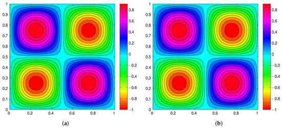
Figure 1.
(a) The contours of an FDEFE solution at and . (b) The contours of an FE solution at and .
In order to show that the RDEFE method is superior to the classical FE method, we also use Problem 3 to calculate four classical FE solutions at and , , , and document the CPU runtime and errors (, , , ), listed on the second and fourth columns in Table 1, where the contours of the FE solution at and are shown in Figure 1b. In the actual engineering calculations, we do not need to find all the classical FE solutions.
By comparing the two photos in Figure 1, we visibly see that Figure 1a and Figure 1b are highly similar, but computing the FDEFE solution saves more computer resource than computing the FE solution.
The data of Table 1 manifest that when (i.e., ) and , , , , the numerical calculating errors to the RDEFE and FE solutions in Table 1 are coincided with the theoretical errors , but the RDEFE method can greatly reduce unknowns and save the CPU runtime because the RDEFE method contains only 6 unknowns during each time iteration, while the FE method contains unknowns during the same time iteration. The data of Table 1 also show that the CPU runtime for computing the RDEFE solutions is far less than that for computing the FE solutions, and it can save time by about a factor of 54. Therefore, the RDEFE method is visibly superior to the FE method.
4.2. Example 2
Assume that , the source function
, and . Thus, Problem 1 has an analytical solution denoted by .
The triangulation on is still formed with the equilateral right triangles with all hypotenuses and all right angles parallel to the axis, , , and . Thus, both the -morn error estimates for the classical FE solutions and the RDEFE solutions for the fractional Tricomi-type equation can also reach according to Theorems 1 and 3, theoretically.
When , , , and , we still find the RDEFE solutions by the following four steps:
(1) By solving Problem 3, based on experience, we also solve out four sets of the first classical FE solution coefficient vectors and , , , ) to construct the snapshot matrix (, , , ).
(2) By resorting to the technique in Section 3.1, we also solve four sets of eigenvalues for the matrix as well as the corresponding set of orthonormal eigenvectors and , , , .
(3) By estimating, we obtain that so that by using the formulas , we also obtain four sets of POD basis vectors (, , , ).
(4) By substituting and the above data into Problem 4, we also calculate four RDEFE solutions at , and document the CPU runtime and errors (, , , ), listed on the third and fifth columns in Table 2.
Table 2.
The errors of the FE and RDEFE solutions and CPU runtime at .
In order to show that the RDEFE method is superior to the classical FE method, we also use Problem 3 to calculate four classical FE solutions at and , , , , and document the CPU runtime and errors (, , , ), listed on the second and fourth columns in Table 2. In the actual engineering calculations, we do not need to find all the classical FE solutions.
The data of Table 2 also manifest that when (i.e., ) and , , , , the numerical calculating errors to the RDEFE and FE solutions are also coincided with the theoretical errors , but the RDEFE method can also lightly reduce unknowns and save the CPU runtime because the RDEFE method also contains only 6 unknowns during each time iteration, while the FE method also contains unknowns during the same time iteration. The data of Table 2 also show that the CPU runtime for finding the RDEFE solutions is much less than that for finding the FE solutions, and it can save time by about a factor of 54. Hence, the RDEFE method is feasible and effective to solve the the fractional Tricomi-type equation.
5. Conclusions and Prospect
Here, we have employed the POD technique to research the dimensionality reduction of the FE method of the fractional Tricomi-type equation. We have established the RDEFE method for the fractional Tricomi-type equation by means of the main POD basis vectors generated by the initial few FE solution vectors. We have also resorted to the matrix analysis to analyze the stability and convergence (errors) of the RDEFE solutions and employed two numerical examples to exhibit the advantages of the RDEFE method. The unknowns for the RDEFE method are far fewer than those for the FE method, so it can not only greatly lighten the calculated burden and lessen the computing error cumulation but also greatly save the CPU runtime in the calculation process. Especially, the dimensionality reduction of the solution vectors to the FE method for the fractional Tricomi-type equation is established for the first time here. Therefore, the RDEFE method for the fractional Tricomi-type equation is brand-new and distinguished from the existing reduced-order/dimension methods, for example, those mentioned in Section 1. This shows that the RDEFE method for the fractional Tricomi-type equation here is a completely new development.
Although only the RDEFE method for the fractional Tricomi-type equation is developed in this paper, the method here can be applied to other unsteady PDEs, even to more complicated real-world engineering problems. Moreover, the RDEFE method in this paper can also generalize to other numerical methods, such as the FD method, collocation method, and meshless method based on thin plate radial basis functions as mentioned in Section 1. Especially, alongside the FE and RDEFE methods, the DG method (see [22,23]) stands out as an efficient alternative for addressing the fractional Tricomi-type problem. This method demonstrates notable efficiency, and its synergy with reduced-dimension extrapolation techniques holds the promise of yielding even more enhanced outcomes. Therefore, the RDEFE method will have a broad application prospect.
Author Contributions
Y.L. and Z.L. contributed to the draft of the manuscript. All authors have read and agreed to the published version of the manuscript.
Funding
This research was supported by the Ordos Science and Technology Plan Project (2022YY041), Inner Mongolia Natural Science Foundation (2019MS06013), and National Natural Science Foundation of China (11671106).
Data Availability Statement
The data presented in this study are available on request from the first author and corresponding author.
Conflicts of Interest
The authors declare no conflict of interest.
References
- Podlubny, I. Fractional Differential Equations; Academic Press: New York, NY, USA, 1999. [Google Scholar]
- Bagley, R.L.; Torvik, P. A theoretical basis for the application of fractional calculus to viscoelasticity. J. Rheol. 1983, 27, 201–210. [Google Scholar] [CrossRef]
- Kilbas, A.A.; Srivastava, H.M.; Trujillo, J.J. Theory and Applications of Fractional Differential Equations; Elsevier Science Limited: Amsterdam, The Netherlands, 2006. [Google Scholar]
- Magin, R.L. Fractional calculus models of complex dynamics in biological tissues. Comput. Math. Appl. 2010, 59, 1586–1593. [Google Scholar] [CrossRef]
- Metzler, R.; Klafter, J. The restaurant at the end of the random walk: Recent developments in the description of anomalous transport by fractional dynamics. J. Phys. A Math. Gen. 2004, 37, R161. [Google Scholar] [CrossRef]
- Miller, K.S.; Ross, B. An Introduction to the Fractional Calculus and Fractional Differential Equations; Wiley: Manhattan, NY, USA, 1993. [Google Scholar]
- Gerasimov, A.N. Generalization of linear deformation laws and their application to problems of internal friction. Prikl. Mat. Mekh. 1948, 12, 529–539. [Google Scholar]
- Caputo, M. Linear model of dissipation whose Q is almost frequency independent, II. Geophys. J. Roy. Astron. Soc. 1967, 13, 529–539. [Google Scholar] [CrossRef]
- Fedorov, V.E.; Zakharova, T.A. Nonlocal solvability of quasilinear degenerate equations with Gerasimov-Caputo derivatives. Lobachevskii J. Math. 2023, 44, 594–606. [Google Scholar] [CrossRef]
- Chen, S.; Liu, F.; Anh, V. A novel implicit finite difference method for the one-dimensional fractional percolation equation. Numer. Algorithms 2011, 56, 517–535. [Google Scholar] [CrossRef]
- Gao, G.; Sun, Z.; Zhang, Y. A finite difference scheme for fractional sub-diffusion equations on an unbounded domain using artificial boundary conditions. J. Comput. Phys. 2012, 231, 2865–2879. [Google Scholar] [CrossRef]
- Vong, S.; Wang, Z. A compact difference scheme for a two dimensional fractional Klein-Gordon equation with neumann boundary conditions. J. Comput. Phys. 2014, 274, 268–282. [Google Scholar] [CrossRef]
- Yuste, S.B.; Acedo, L. An explicit finite difference method and a new von neumann-type stability analysis for fractional diffusion equations. SIAM J. Numer. Anal. 2005, 42, 1862–1874. [Google Scholar] [CrossRef]
- Zeng, F.; Zhang, Z.; Karniadakis, G.E. Fast difference schemes for solving high-dimensional time-fractional subdiffusion equations. J. Comput. Phys. 2016, 307, 15–33. [Google Scholar] [CrossRef]
- Dehghan, M.; Abbaszadeh, M. An efficient technique based on finite difference/finite element method for solution of two-dimensional space/multi-time fractional bloch-torrey equations. Appl. Numer. Math. 2018, 131, 190–206. [Google Scholar] [CrossRef]
- Dehghan, M.; Safarpoor, M.; Abbaszadeh, M. Two high-order numerical algorithms for solving the multi-term time fractional diffusion-wave equations. J. Comput. Appl. Math. 2015, 290, 174–195. [Google Scholar] [CrossRef]
- Jiang, Y.; Ma, J. High-order finite element methods for time-fractional partial differential equations. J. Comput. Appl. Math. 2011, 235, 3285–3290. [Google Scholar] [CrossRef]
- Liu, Q.; Liu, F.; Turner, I.; Anh, V. Finite element approximation for a modified anomalous subdiffusion equation. Appl. Math. Model. 2011, 35, 4103–4116. [Google Scholar] [CrossRef]
- Baseri, A.; Abbasbandy, S.; Babolian, E. A collocation method for fractional diffusion equation in a long time with chebyshev functions. Appl. Math. Comput. 2018, 322, 55–65. [Google Scholar] [CrossRef]
- Esen, A.; Tasbozan, O.; Ucar, Y.; Yagmurlu, N. A b-spline collocation method for solving fractional diffusion and fractional diffusion-wave equations. Tbilisi. Math. J. 2015, 8, 181–193. [Google Scholar] [CrossRef]
- Nagy, A. Numerical solution of time fractional nonlinear Klein-Gordon equation using sinc-Chebyshev collocation method. Appl. Math. Comput. 2017, 310, 139–148. [Google Scholar] [CrossRef]
- Xu, Q.; Hesthaven, J.S. Discontinuous Galerkin Method for Fractional Convection-Diffusion Equations. SIAM J. Numer. Anal. 2014, 52, 405–423. [Google Scholar] [CrossRef]
- Baccouch, M.; Temimi, H. A high-order space-time ultra-weak discontinuous Galerkin method for the second-order wave equation in one space dimension. J. Comput. Appl. Math. 2021, 389, 113331. [Google Scholar] [CrossRef]
- Bhardwaj, A.; Kumar, A. Numerical solution of time fractional Tricomi-type equation by an RBF based meshless method. Eng. Anal. Bound. Elem. 2020, 118, 96–107. [Google Scholar] [CrossRef]
- Liu, F.; Anh, V.; Turner, I.; Zhang, P. Time fractional advection dispersion equation. J. Appl. Math. Comput. 2003, 13, 233–245. [Google Scholar] [CrossRef]
- Lin, Y.M.; Xu, C.J. Finite difference/spectral approximations for the time-fractional diffusion equation. J. Comput. Phys. 2007, 225, 1533–1552. [Google Scholar] [CrossRef]
- Ervin, V.J.; Roop, J.P. Variational formulation for the stationary fractional advection dispersion equation. Numer. Methods Part. Differ. Equ. 2006, 22, 558–576. [Google Scholar] [CrossRef]
- Zhang, H.; Liu, F.; Anh, V. Galerkin finite element approximations of symmetric space fractional partial differnetial equations. Appl. Math. Comput. 2010, 217, 2534–2545. [Google Scholar]
- Li, C.P.; Zhao, Z.G.; Chen, Y.Q. Numerical approximation of nonlinear fractional differential equations with subdiffusion and superdiffusion. Comput. Math. Appl. 2011, 62, 855–875. [Google Scholar] [CrossRef]
- Ford, N.J.; Xiao, J.Y.; Yan, Y.B. A finite element method for time fractional partial differential equations. Fract. Calc. Appl. Anal. 2011, 14, 454–474. [Google Scholar] [CrossRef]
- Zhang, X.D.; Huang, P.Z.; Feng, X.L.; Wei, L.L. Finite element method for two-dimensional time-fractional Tricomi-type equations. Numer. Methods Part. Differ. Equ. 2013, 29, 1081–1096. [Google Scholar] [CrossRef]
- Alekseev, A.K.; Bistrian, D.A.; Bondarev, A.E.; Navon, I.M. On linear and nonlinear aspects of dynamic mode decomposition. Int. J. Numer. Meth. Fluids 2016, 82, 348–371. [Google Scholar] [CrossRef]
- Aubry, N.; Holmes, P.; Lumley, J.L.; Stone, E. The dynamics of coherent structures in the wall region of a turbulent boundary layer. J. Fluid Mech. 1988, 192, 115–173. [Google Scholar] [CrossRef]
- Du, J.; Navon, I.M.; Zhu, J.; Fang, F.; Alekseev, A.K. Reduced order modeling based on POD of a parabolized Navier-Stokes equations model II. Trust region POD 4D VAR data assimilation. Comput. Math. Appl. 2013, 65, 380–394. [Google Scholar] [CrossRef]
- Ghaffari, R.; Ghoreishi, F. Reduced spline method based on a proper orthogonal decomposition technique for fractional sub-diffusion equations. Appl. Numer. Math. 2019, 137, 62–79. [Google Scholar] [CrossRef]
- Hinze, M.; Kunkel, M. Residual based sampling in POD model order reduction of drift-diffusion equations in parametrized electrical networks. J. Appl. Math. Mech. 2012, 92, 91–104. [Google Scholar] [CrossRef]
- Li, H.R.; Song, Z.Y. A reduced-order energy-stability-preserving finite difference iterative scheme based on POD for the Allen-Cahn equation. J. Math. Anal. Appl. 2020, 491, 124245. [Google Scholar] [CrossRef]
- Li, H.R.; Song, Z.Y. A reduced-order finite element method based on proper orthogonal decomposition for the Allen-Cahn model. J. Math. Anal. Appl. 2021, 500, 125103. [Google Scholar] [CrossRef]
- Luo, Z.D.; Chen, G. Proper Orthogonal Decomposition Methods for Partial Differential Equations; Academic Press of Elsevier: San Diego, CA, USA, 2018. [Google Scholar]
- Luo, Z.D.; Yang, J. The reduced-order method of continuous space-time finite element scheme for the non-stationary incompressible flows. J. Comput. Phys. 2022, 456, 111044. [Google Scholar] [CrossRef]
- Song, Z.Y.; Li, H.R. Numerical simulation of the temperature field of the stadium building foundation in frozen areas based on the finite element method and proper orthogonal decomposition technique. Math. Method. Appl. Sci. 2021, 44, 8528–8542. [Google Scholar] [CrossRef]
- Luo, Z.D. The reduced-order extrapolating method about the Crank–Nicolson finite element solution coefficient vectors for parabolic type equation. Mathematics 2020, 8, 1261. [Google Scholar] [CrossRef]
- Luo, Z.D. The dimensionality reduction of Crank–Nicolson mixed finite element solution coefficient vectors for the unsteady Stokes equation. Mathematics 2022, 10, 2273. [Google Scholar] [CrossRef]
- Luo, Z.D.; Jiang, W.R. A reduced-order extrapolated technique about the unknown coefficient vectors of solutions in the finite element method for hyperbolic type equation. Appl. Numer. Math. 2020, 158, 123–133. [Google Scholar] [CrossRef]
- Teng, F.; Luo, Z.D. A reduced-order extrapolation technique for solution coefficient vectors in the mixed finite element method for the 2D nonlinear Rosenau equation. J. Math. Anal. Appl. 2020, 385, 123761. [Google Scholar] [CrossRef]
- Zeng, Y.H.; Luo, Z.D. The reduced-order technique about the unknown solution coefficient vectors in the Crank-Nicolson finite element algorithm for the Sobolev equation. J. Math. Anal. Appl. 2022, 513, 126207. [Google Scholar] [CrossRef]
- Liu, J.C.; Li, H.; Liu, Y.; Fang, Z.C. Reduced-order finite element method based on POD for fractional Tricomi-type equation. Appl. Math. Mech. 2016, 37, 647–658. [Google Scholar] [CrossRef]
- Zhang, G.; Lin, Y. Notes on Functional Analysis; Peking University Press: Beijing, China, 1987. (In Chinese) [Google Scholar]
- Zhang, W.S. Finite Difference Methods for Partial Differential Equations in Science Computation; Higher Education Press: Beijing, China, 2006. (In Chinese) [Google Scholar]
- Luo, Z.D. The Foundations and Applications of Mixed Finite Element Methods; Chinese Science Press: Beijing, China, 2006. (In Chinese) [Google Scholar]
Disclaimer/Publisher’s Note: The statements, opinions and data contained in all publications are solely those of the individual author(s) and contributor(s) and not of MDPI and/or the editor(s). MDPI and/or the editor(s) disclaim responsibility for any injury to people or property resulting from any ideas, methods, instructions or products referred to in the content. |
© 2023 by the authors. Licensee MDPI, Basel, Switzerland. This article is an open access article distributed under the terms and conditions of the Creative Commons Attribution (CC BY) license (https://creativecommons.org/licenses/by/4.0/).