A General Case of a Line Contact Lubricated by a Non-Newtonian Giesekus Fluid

Abstract

A steady plane hydrodynamic problem of lubrication of a lightly loaded contact of two parallel cylinders lubricated by a non-Newtonian fluid with Giesekus rheology is considered. The advantage of this non-Newtonian rheology is its ability to properly describe the real behavior of formulated lubricants at high and low shear stresses. The problem is solved by using a modification of the regular perturbation method with respect to the small parameter $\alpha$, characterizing the degree to which the polymeric molecules of the additive to the lubricant follow the streamlines of the lubricant flow. It is assumed that the lubricant relaxation time and the value of $\alpha$ are of the order of the magnitude of the ratio of the characteristic gap between the contact surfaces and the contact length. The obtained analytical solution of the problem is analyzed numerically for the dependencies of the problem characteristics such as contact pressure, fluid flux, lubrication film thickness, friction force, energy loss in the lubricated contact, etc., on the problem input parameters.

1. Introduction

Most machine elements work in lubricated environments. Generally, the usage of lubrication allows a decrease in frictional losses in contacts and, thus, an increase in their durability. When such lubricated contacts are mathematically modeled, the rheology of the lubricant is considered to be Newtonian or non-Newtonian. The former case is significantly simpler and a lot of studies for the cases of homogeneous material and coated solids [1,2,3,4,5,6,7,8,9,10] were dedicated to it. The latter case is more complex, but it better corresponds to the real behavior of lubricants because polymeric additives make their behavior significantly non-Newtonian, which allows for a distinctly different lubricant behavior at low and high shear stresses. Different rheological models for lubricant behavior were used to catch various aspects of real lubricant behavior such as lubricant relaxation time, etc. An overview and analysis of different fluid rheological models is given in [11,12]. One of the simplest rheological models of non-Newtonian lubricant behavior among generalized Newtonian fluids [13] is the Ree–Eyring model [14,15,16]. Some studies of fluids with complex non-Newtonian rheology were presented in [17,18,19,20,21,22].

Experimental data show that lubricant viscosity depends not only on pressure but also on lubricant shear stress and velocity [23]. The actual behavior of polymer-formulated lubricant flowing through narrow gaps is most accurately described by the Giesekus rheological model [12,24,25]. The Giesekus model differs from the Maxwell, Jeffris, Oldroyd A and B, etc., rheological models by the presence of a nonlinear term determined by the mobility factor $\alpha$ and stress state of the fluid. It provides the opportunity to take into account the degree to which the fluid viscosity is dependent on the shear stress in the fluid. In particular, this model allows for proper accounting of relatively high viscosity for low and relatively low viscosity for high shear stresses in the fluid. The model takes into account four parameters of the fluid: the relaxation time, the viscosities of base oil and polymeric additive and the mobility factor. If the mobility factor is set to zero, then the Giesekus model turns into the convected Maxwell model [11,12]. The Giesekus model is nonlinear and, therefore, more complex for analysis. A relatively simple case of a fluid with Giesekus rheology flowing between two parallel surfaces is considered in [26,27]. In [28], the analysis of a lightly loaded trust bearing lubricated by a fluid with the Giesekus rheology was performed by the perturbation methods. However, the presence of convective terms and the base oil were not taken into account.

The present paper is the continuation of the series of the author’s studies of hydro- and elastohydrodynamic problems for Newtonian [29,30] and non-Newtonian [13] lubricating fluids including the study of a lightly loaded trust bearing lubricated with a fluid with the Giesekus rheology [31]. Also, the authors previously considered a similar but more simple problem under the condition when the mobility factor $\alpha$ is significantly greater than the ratio of the characteristic gap between the surfaces and length of the contact [32]. In this case, in a two-term asymptotic solution, the inertia terms can be neglected. The first two terms of asymptotic representation for contact pressure with respect to the small parameter $\alpha$ are obtained in the analytical form. Numerical analysis of the obtained relationships for contact pressure, lubrication film thickness, lubricant flux, friction, contact energy loss, etc., as functions of the input parameters of the Giesekus model is performed. Some applications of perturbation methods to steady problems similar to the one used are described in [33,34].

2. Formulation of the Lubrication Problem and General Description of the Analysis Applied

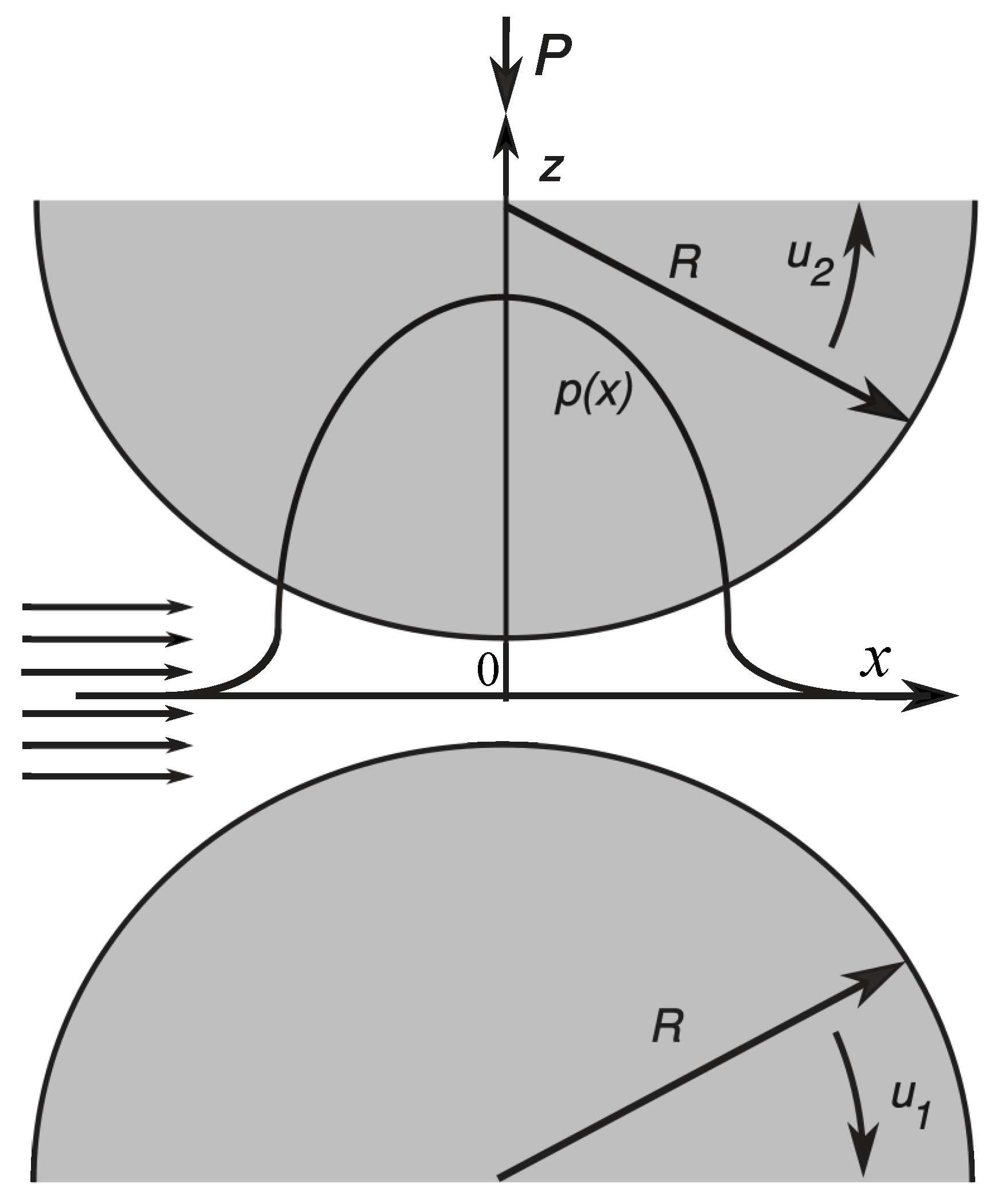
Let us consider a steady plane problem for a lubricated contact of two parallel infinite cylinders of the radius R (see Figure 1), both of which are made of rigid materials (the case of cylinders of different radii is considered at the end of the paper). It is assumed that the lubricant is described by the Giesekus model [12] with a constant viscosity $\mu$ and relaxation time ${\lambda }_1$. The x-axis of the coordinate system is directed along the contact and perpendicular to the cylinder axes, the y-axis is directed along the cylinder axes, and the z-axis is perpendicular to both x- and y-axes. A continuous lubricant layer separates the cylinders which steadily roll and slide with the surface linear speeds $\overline{u_1}$ and $\overline{u_2}$ in the direction of the x-axis. The upper cylinder is subjected to the normal load P along the z-axis. The lubricant velocity components are represented by functions $u(x,y,z),v(x,y,z)$, and $w(x,y,z)$. Due to the problem geometry, $v(x,y,z)=\frac{\partial v(x,y,z)}{\partial y}=0.$ Therefore, the problem parameters are independent of y and the motion equations of such a fluid are as follows [13,29].

$$\begin{array}{c}u\frac{\partial u}{\partial x}+w\frac{\partial u}{\partial z}=\frac{1}{\rho }(\frac{\partial p_{xx}}{\partial x}+\frac{\partial p_{zx}}{\partial z}),\frac{\partial p_{xy}}{\partial x}+\frac{\partial p_{zy}}{\partial z}=0,\\ \\ u\frac{\partial w}{\partial x}+w\frac{\partial w}{\partial z}=\frac{1}{\rho }(\frac{\partial p_{zx}}{\partial x}+\frac{\partial p_{zz}}{\partial z}).\end{array}$$

(1)

In addition to that, one needs to consider the continuity equation. It is assumed that the fluid is incompressible, i.e., $\rho (x,z)=constant$. That leads to the continuity equation

$$\begin{array}{c}\frac{\partial u}{\partial x}+\frac{\partial w}{\partial z}=0.\end{array}$$

(2)

In this case, the stress tensor components are as follows

$$\begin{array}{c}{p}_{xx}=-p+{\tau }_{xx},p_{xy}={\tau }_{xy}=0,p_{zx}={\tau }_{zx},p_{zz}=-p+{\tau }_{zz},p_{zy}={\tau }_{zy}=0,\end{array}$$

(3)

where p is the pressure and ${\tau }_{xx},{\tau }_{xy},{\tau }_{zx},{\tau }_{zz},$ and ${\tau }_{zy}$ are the additional stress components acting in the corresponding directions. These tensor components satisfy the Giesekus fluid model which is a certain generalization of the Maxwell model and takes into account the degree to which the additive polymeric molecules follow the lubricant flow. The rheological equations are as follows [12]

$$\begin{array}{c}\tau ={\tau }_s+{\tau }_p,\mu ={\mu }_s+{\mu }_p,{\tau }_s={\mu }_s\dot{\gamma },\\ \\ {\tau }_p+{\lambda }_1{\tau }_{p\left(1\right)}-\alpha \frac{{\lambda }_1}{{\mu }_p}\{{\tau }_p·{\tau }_p\}={\mu }_p\dot{\gamma },\end{array}$$

(4)

where $\tau$ is the full stress tensor while ${\tau }_s$ and ${\tau }_p$ are the solvent and polymer stress tensors, respectively, ${\mu }_s$ and ${\mu }_p$ are the constant solvent and polymer dynamic viscosities, $\dot{\gamma }$ is the deformation tensor, ${\lambda }_1$ is the constant relaxation time, and $\alpha$ is the dimensionless constant mobility factor describing the degree of the alignment of polymeric molecules with the lubricant flow, $0\le \alpha \le 1$.

In (4), the following definitions of the tensor operators ${\tau }_{p\left(1\right)}$ and $\{{\tau }_p·{\tau }_p\}$ [12] are used

$$\begin{array}{c}{\tau }_{p\left(1\right)xx}=u\frac{\partial {\tau }_{pxx}}{\partial x}+w\frac{\partial {\tau }_{pxx}}{\partial z}-2\frac{\partial u}{\partial z}{\tau }_{pxz}-2\frac{\partial u}{\partial x}{\tau }_{pxx},\\ \\ {\tau }_{p\left(1\right)xz}=u\frac{\partial {\tau }_{pxz}}{\partial x}+w\frac{\partial {\tau }_{pxz}}{\partial z}-\frac{\partial u}{\partial x}{\tau }_{pzx}-\frac{\partial u}{\partial z}{\tau }_{pzz}-\frac{\partial w}{\partial x}{\tau }_{pxx}-\frac{\partial w}{\partial z}{\tau }_{pzx},\\ \\ {\tau }_{p\left(1\right)zz}=u\frac{\partial {\tau }_{pzz}}{\partial x}+w\frac{\partial {\tau }_{pzz}}{\partial z}-2\frac{\partial w}{\partial z}{\tau }_{pzz}-2\frac{\partial w}{\partial x}{\tau }_{pzx},\\ \\ {\{{\tau }_p·{\tau }_p\}}_{xx}={\tau }_{pxx}^2+{\tau }_{pxz}^2,\\ \\ {\{{\tau }_p·{\tau }_p\}}_{xz}={\tau }_{pxx}{\tau }_{pxz}+{\tau }_{pxz}{\tau }_{pzz},\\ \\ {\{{\tau }_p·{\tau }_p\}}_{zz}={\tau }_{pxz}^2+{\tau }_{pzz}^2.\end{array}$$

(5)

and [12]

$$\begin{array}{c}{\dot{\gamma }}_{xx}=2\frac{\partial u}{\partial x},{\dot{\gamma }}_{xz}=\frac{\partial u}{\partial z}+\frac{\partial w}{\partial x},{\dot{\gamma }}_{zz}=2\frac{\partial w}{\partial z}.\end{array}$$

(6)

It is necessary to impose some boundary conditions on the components u and w of the lubricant velocity on the surfaces of the contacting solids. It is assumed that the no-slip and no-penetration conditions are valid on the solid boundaries. The contact is considered to be concentrated, i.e., $L_z/L_x\ll 1$ (where $L_x$ and $L_z$ are the characteristic contact sizes along the x- and z-axes) or equivalently $dh\left(x\right)/dx\ll 1$, where $h\left(x\right)$ is the gap between the cylinder surfaces at point x. Using the above boundary conditions will take the form

$$\begin{array}{c}u(x,-\frac{h(x)}{2})=\overline{u_1},u(x,\frac{h(x)}{2})=\overline{u_2},\end{array}$$

(7)

$$\begin{array}{c}w(x,-\frac{h(x)}{2})=-\frac{\overline{u_1}}{2}\frac{dh(x)}{dx},w(x,\frac{h(x)}{2})=\frac{\overline{u_2}}{2}\frac{dh(x)}{dx}.\end{array}$$

(8)

It will be shown later that in the simplified formulation the function of pressure p is independent of the variable z. Therefore, under pressure, one can impose the boundary conditions stemming from the fact that at the contact boundaries the fluid pressure p is equal to the atmospheric one and, therefore, can be neglected. To avoid cavitation at the exit from the contact [13], the boundary conditions on p have the form

$$\begin{array}{c}p\left(x_i\right)=p\left(x_e\right)=\frac{dp\left(x_e\right)}{dx}=0,\end{array}$$

(9)

where $x_i$ and $x_e$ are the coordinates of the inlet and exit points of the contact.

In addition to that, it is required that the stress $-p_{zz}$ from (3) supports the normal load P applied to the cylinder, i.e.,

$$\begin{array}{c}\underset{x_i}{\overset{x_e}{\int }}[p\left(x\right)-{\tau }_{zz}(x,h\left(x\right)/2)]dx=P.\end{array}$$

(10)

Being interested in a two-term asymptotic problem solution in $\alpha$, in (9) and (10), it is assumed that the two-term asymptotic expansion of pressure $p(x,z)$ in $\alpha$ (i.e., a linear function of $\alpha$) is independent of z. That assumption is confirmed later for small $\alpha$ up to the order of $O\left(\alpha \right),\alpha \ll 1$, i.e., in the asymptotic expansion of p in $\alpha \ll 1$, terms $p_0$ and $p_1$ are independent of z, while terms $p_2,p_3,\dots$ depend on both x and z.

The goal is to determine the contact pressure $p\left(x\right)$, the gap between the two cylinders $h\left(x\right)$, the coordinate of the exit point from the lubricated contact $x_e$, the components of the tensor $\tau$ in the fluid, etc. Typically, the point of entrance in the lubricated contact, i.e., the coordinate of the inlet point $x_i$, is known, and it is determined by the amount of lubricant supplied to the contact. The region where the problem solution is searched is bounded by $x=x_i$ and $x=x_e$ as well as by $z=-h\left(x\right)/2$ and $z=h\left(x\right)/2$. Out of these four boundaries of the region, three are unknown, i.e., $x=x_e$, $z=-h\left(x\right)/2$, and $z=h\left(x\right)/2$ are unknown. One needs to find a perturbation solution to the above-determined problem in the case when $\alpha \ll 1$. In this case, $x_e$ and $h\left(x\right)$ are just slightly perturbed values of the exit point $x_{e0}$ and gap $h_0\left(x\right)$ realized in a lubricated contact with Newtonian fluid, i.e., when $\alpha =0$.

The general case of

$$\begin{array}{c}\alpha ={\alpha }_0ϵ,{\alpha }_0=O\left(1\right),ϵ=\frac{L_z}{L_x}\ll 1,\end{array}$$

(11)

will be considered. Here, ${\alpha }_0$ is a nonnegative constant. This case allows us to take into account some of the convective as well as major and minor dissipative terms of the equations. Also, it allows us to consider the limiting cases $\alpha \gg ϵ$ and $\alpha \ll ϵ$ by correspondingly taking ${\alpha }_0\gg 1$ and ${\alpha }_0\ll 1$.

3. Simplification of the Rheological Equations and the Equations of Lubricant Motion

It was shown that the problem solution should be searched for not in the original $(x,z)$ independent variables but in slightly modified ones $(x_0,z_0)$. It is due to the fact that the exit $x=x_e$ and upper $z=h\left(x\right)/2$ and lower $z=-h\left(x\right)/2$ boundaries of the lubricated contact are perturbed ones of the corresponding boundaries $x=x_{e0}$ and $z=\pm h_0\left(x_0\right)/2$ of the contact lubricated by a Newtonian fluid (for $\alpha =0$). Therefore, let us assume that

$$\begin{array}{c}{x}_e=x_{e0}+\alpha x_{e1}+\dots ,h\left(x\right)=h_0\left(x_0\right)+\alpha h_1\left(x_0\right)+\dots ,\end{array}$$

(12)

where $x_{e1}$ and $h_1\left(x_0\right)$ will be determined as a part of the problem solution. Then, the problem can be projected on the region $[x_i,x_{e0}]\times [-h_0\left(x_0\right)/2,h_0\left(x_0\right)/2]$ by introducing the following new independent variables

$$\begin{array}{c}x=x_0+\alpha x_{e1}\frac{x_0-x_i}{x_{e0}-x_i},z=\frac{h\left(x\right)}{h_0\left(x_0\right)}{z}_0.\end{array}$$

(13)

When $x_0=x_i$ and $x_0=x_{e0}$ with the precision of $O\left({\alpha }^2\right),\alpha \ll 1$, one obtains $x=x_i$ and $x=x_e$, respectively, and vice versa (see (12) and (13)). The actual definition of the new variable $x_0$ can be taken as $x_0=(x_i+x_{e0})/2+\xi (x_{e0}-x_i)/2,-1\le \xi \le 1$, which varies between $x_i$ and $x_{e0}$.

As it was shown earlier, this projection of the original problem onto the region $[x_i,x_{e0}]\times [-h_0\left(x_0\right)/$$2,h_0\left(x_0\right)/2]$ is also dictated by the asymptotic expansion of the boundary conditions on pressure $p\left(x\right)$ at the exit point $x=x_e$ [31,32].

Let us consider the solution form which should be used in this case. One needs to modify integration and differentiation operators while converting the problem from variables $(x,z)$ to variables $(x_0,z_0)$ as follows (see (12) and (13))

$$\begin{array}{c}dx=[1+\alpha \frac{x_{e1}}{x_{e0}-x_i}+\dots ]d{x}_0,dz=[1+\alpha \frac{h_1(x_0)}{h_0(x_0)}+\dots ]d{z}_0,\\ \\ \frac{\partial }{\partial x}=[1-\alpha \frac{x_{e1}}{x_{e0}-x_i}+\dots ]\frac{\partial }{\partial x_0},\frac{\partial }{\partial z}=[1-\alpha \frac{h_1(x_0)}{h_0(x_0)}+\dots ]\frac{\partial }{\partial z_0}.\end{array}$$

(14)

Let us consider an arbitrary sufficiently smooth function $f(\alpha ,x,z)$ which has to be expanded asymptotically in $\alpha \ll 1$. Then, based on (12) and (13), one has [31,32]

$$\begin{array}{c}f(\alpha ,x,z)=f(0,x,z)+\alpha f_{1*}(x,z)+\dots \\ \\ =f(0,x_0+\frac{\alpha x_{e1}(x_0-x_i)}{x_{e0}-x_i}+\dots ,\frac{(h_0(x_0)+\alpha h_1(x_0)+\dots )z_0}{h_0(x_0)})\\ \\ +\alpha f_{1*}(x_0+\frac{\alpha x_{e1}(x_0-x_i)}{x_{e0}-x_i}+\dots ,\frac{(h_0(x_0)+\alpha h_1(x_0)+\dots )z_0}{h_0(x_0)})+\dots \\ \\ =f(0,x_0,z_0)+\alpha [f_1(x_0,z_0)+\frac{x_{e1}(x_0-x_i)}{x_{e0}-x_i}\frac{\partial f(0,x_0,z_0)}{\partial x_0}+\frac{z_0{h}_1(x_0)}{h_0(x_0)}\frac{\partial f(0,x_0,z_0)}{\partial z_0}]+\dots ,\end{array}$$

(15)

where $f_{1*}(x,z)=\frac{\partial f(0,x,z)}{\partial \alpha }$ and the derivative of f with respect to $x_0$ and $z_0$ are also taken for $\alpha =0$. Therefore, the solution of the problem one will search using the Taylor expansions of the unknown functions such as $p\left(x\right)$, $u(x,z)$, ${\tau }_{xx}(x,z)$, etc., about $x_0$ and $(x_0,z_0)$, retaining just the first two terms of the expansions as well as taking into account the sample expansion (15) and the perturbed expressions for $x_e$ and $h\left(x\right)$ from (12) and (13).

In the form the problem is formulated above it is very complex for any analytical analysis except the perturbation method. Therefore, the first goal is to simplify Equations (1)–(8) and to reduce them to much simpler equations which would allow for an analytical solution and derivation of analogs of the Reynolds equation. One needs to retain only the terms of higher orders of magnitude. As it was mentioned earlier, due to the fact that the thickness of the lubrication layer is much smaller than the extent of the lubricated contact, one has a small parameter $ϵ=L_z/L_x\ll 1$. Also, let $U_x$ and $U_z$ be the characteristic velocities of the lubricating fluid in the directions of the x- and z-axes. Then, the following scaling of the equations can be introduced

$$\begin{array}{c}{\lambda }_1^{\prime }=\frac{U_x}{L_x}{\lambda }_1,x^{\prime }=\frac{x}{L_x},z^{\prime }=\frac{z}{L_z},p^{\prime }=p\frac{L_z^2}{{\mu }_{*}{U}_x{L}_x},\\ \\ u^{\prime }=\frac{u}{U_x},w^{\prime }=\frac{w}{U_z},s_0=2\frac{\overline{u_2}-\overline{u_1}}{\overline{u_1}+\overline{u_2}},\{{\mu }^{\prime },{\mu }_s^{\prime },{\mu }_p^{\prime }\}=\frac{1}{{\mu }_{*}}\{\mu ,{\mu }_s,{\mu }_p\},\\ \\ \{{\tau }_{xx}^{\prime },{\tau }_{sxx}^{\prime },{\tau }_{pxx}^{\prime },{\tau }_{zx}^{\prime },{\tau }_{szx}^{\prime },{\tau }_{pzx}^{\prime },{\tau }_{zz}^{\prime },{\tau }_{szz}^{\prime },{\tau }_{pzz}^{\prime }\}=\frac{L_z\{{\tau }_{xx},{\tau }_{sxx},{\tau }_{pxx},{\tau }_{zx},{\tau }_{szx},{\tau }_{pzx},{\tau }_{zz},{\tau }_{szz},{\tau }_{pzz}\}}{{\mu }_{*}{U}_x},\end{array}$$

(16)

where ${\mu }_{*}$ is the characteristic value of the lubricant viscosity. For simplicity, in the further analysis, the primes at the dimensionless variables are dropped.

By introducing the above scaling in the continuity Equation (2), one obtains

$$\begin{array}{c}\frac{\partial u}{\partial x}+\frac{U_z}{U_x}\frac{L_x}{L_z}\frac{\partial w}{\partial z}=0.\end{array}$$

(17)

To retain both terms in Equation (17), one needs to assume that

$$\begin{array}{c}\frac{U_z}{U_x}\frac{L_x}{L_z}=1.\end{array}$$

(18)

Then, Equation (17) becomes

$$\begin{array}{c}\frac{\partial u}{\partial x}+\frac{\partial w}{\partial z}=0.\end{array}$$

(19)

Introducing scaling (16) in Equations (1) and (3)–(6) leads to equations

$$\begin{array}{c}ϵR{e}_0\{u\frac{\partial u}{\partial x}+w\frac{\partial u}{\partial z}\}=-\frac{\partial p}{\partial x}+ϵ\frac{\partial {\tau }_{xx}}{\partial x}+\frac{\partial {\tau }_{zx}}{\partial z},\\ \\ {ϵ}^{3}R{e}_0\{u\frac{\partial w}{\partial x}+w\frac{\partial w}{\partial z}\}={ϵ}^2\frac{\partial {\tau }_{zx}}{\partial x}-\frac{\partial p}{\partial z}+ϵ\frac{\partial {\tau }_{zz}}{\partial z},\end{array}$$

(20)

$$\begin{array}{c}{\tau }_{xx}={\tau }_{sxx}+{\tau }_{pxx},{\tau }_{zx}={\tau }_{szx}+{\tau }_{pzx},{\tau }_{zz}={\tau }_{szz}+{\tau }_{pzz},{\tau }_{sxx}=ϵ2{\mu }_s\frac{\partial u}{\partial x},\\ \\ {\tau }_{szx}={\mu }_s({ϵ}^2\frac{\partial w}{\partial x}+\frac{\partial u}{\partial z}),{\tau }_{szz}=ϵ2{\mu }_s\frac{\partial w}{\partial z}=-ϵ2{\mu }_s\frac{\partial u}{\partial x},\end{array}$$

(21)

$$\begin{array}{c}{\tau }_{pxx}+{\lambda }_1[u\frac{\partial {\tau }_{pxx}}{\partial x}+w\frac{\partial {\tau }_{pxx}}{\partial z}-\frac{2}{ϵ}\frac{\partial u}{\partial z}{\tau }_{pzx}-2\frac{\partial u}{\partial x}{\tau }_{pxx}]-\alpha \frac{{\lambda }_1}{ϵ{\mu }_p}({\tau }_{pxx}^2+{\tau }_{pzx}^2)=2ϵ{\mu }_p\frac{\partial u}{\partial x},\\ \\ {\tau }_{pzx}+{\lambda }_1[u\frac{\partial {\tau }_{pzx}}{\partial x}+w\frac{\partial {\tau }_{pzx}}{\partial z}-\frac{1}{ϵ}\frac{\partial u}{\partial z}{\tau }_{pzz}-\frac{\partial u}{\partial x}{\tau }_{pzx}-\frac{\partial w}{\partial z}{\tau }_{pzx}-ϵ\frac{\partial w}{\partial x}{\tau }_{pxx}]\\ \\ -\alpha \frac{{\lambda }_1}{ϵ{\mu }_p}({\tau }_{pxx}+{\tau }_{pzz}){\tau }_{pzx}={\mu }_p(\frac{\partial u}{\partial z}+{ϵ}^2\frac{\partial w}{\partial x}),\\ \\ {\tau }_{pzz}+{\lambda }_1[u\frac{\partial {\tau }_{pzz}}{\partial x}+w\frac{\partial {\tau }_{pzz}}{\partial z}-2\frac{\partial w}{\partial z}{\tau }_{pzz}-2ϵ\frac{\partial w}{\partial x}{\tau }_{pzx}]-\alpha \frac{{\lambda }_1}{ϵ{\mu }_p}({\tau }_{pzx}^2+{\tau }_{pzz}^2)=2ϵ{\mu }_p\frac{\partial w}{\partial z},\end{array}$$

(22)

where $R{e}_0=\frac{\rho U_x{L}_z}{{\mu }_{*}}$ is the local Reynolds number.

Let us assume that not only $ϵ\ll 1$ but also $R{e}_0=O\left(1\right),\alpha \ll 1$, and

$$\begin{array}{c}{\lambda }_1=\lambda ϵ,\lambda =O\left(1\right),ϵ\ll 1.\end{array}$$

(23)

The latter assumption makes the rheological equations solvable. Otherwise, for ${\lambda }_1=O\left(1\right)$, $ϵ\ll 1$, these equations do not have a reasonable solution.

Then, Equations (20)–(22) can be simplified. Based on the example of function $f(\alpha ,x,z)$ expansion for $\alpha \ll 1$, one needs to search the problem solution in the form

$$\begin{array}{c}\{{\tau }_{sxx}(x,z),{\tau }_{sxz}(x,z),{\tau }_{szz}(x,z)\}=\{{\tau }_{sxx0}(x_0,z_0),{\tau }_{sxz0}(x_0,z_0),{\tau }_{szz0}(x_0,z_0)\}\\ \\ +\alpha \{{\tau }_{sxx1*}(x_0,z_0),{\tau }_{sxz1*}(x_0,z_0),{\tau }_{szz1*}(x_0,z_0)\}+\cdots ,\\ \\ \{{\tau }_{sxx1*}(x_0,z_0),{\tau }_{sxz1*}(x_0,z_0),{\tau }_{szz1*}(x_0,z_0)\}\\ \\ =\{{\tau }_{sxx1}(x_0,z_0),{\tau }_{sxz1}(x_0,z_0),{\tau }_{szz1}(x_0,z_0)\}\\ \\ +x_{e1}\frac{x_0-x_i}{x_{e0}-x_i}\frac{\partial }{\partial x_0}\{{\tau }_{sxx0}(x_0,z_0),{\tau }_{sxz0}(x_0,z_0),{\tau }_{szz0}(x_0,z_0)\}\\ \\ +z_0\frac{h_1\left(x_0\right)}{h_0\left(x_0\right)}\frac{\partial }{\partial z_0}\{{\tau }_{sxx0}(x_0,z_0),{\tau }_{sxz0}(x_0,z_0),{\tau }_{szz0}(x_0,z_0)\},\end{array}$$

(24)

$$\begin{array}{c}\{{\tau }_{pxx}(x,z),{\tau }_{pxz}(x,z),{\tau }_{pzz}(x,z)\}=\{{\tau }_{pxx0}(x_0,z_0),{\tau }_{pxz0}(x_0,z_0),{\tau }_{pzz0}(x_0,z_0)\}\\ \\ +\alpha \{{\tau }_{pxx1*}(x_0,z_0),{\tau }_{pxz1*}(x_0,z_0),{\tau }_{pzz1*}(x_0,z_0)\}+\dots ,\\ \\ \{{\tau }_{pxx1*}(x_0,z_0),{\tau }_{pxz1*}(x_0,z_0),{\tau }_{pzz1*}(x_0,z_0)\}\\ \\ =\{{\tau }_{pxx1}(x_0,z_0),{\tau }_{pxz1}(x_0,z_0),{\tau }_{pzz1}(x_0,z_0)\}\\ \\ +x_{e1}\frac{x_0-x_i}{x_{e0}-x_i}\frac{\partial }{\partial x_0}\{{\tau }_{pxx0}(x_0,z_0),{\tau }_{pxz0}(x_0,z_0),{\tau }_{pzz0}(x_0,z_0)\}\\ \\ +z_0\frac{h_1\left(x_0\right)}{h_0\left(x_0\right)}\frac{\partial }{\partial z_0}\{{\tau }_{pxx0}(x_0,z_0),{\tau }_{pxz0}(x_0,z_0),{\tau }_{pzz0}(x_0,z_0)\},\end{array}$$

(25)

$$\begin{array}{c}p\left(x\right)=p_0\left(x_0\right)+\alpha p_{1*}\left(x_0\right)+\dots ,\\ \\ p_{1*}\left(x_0\right)=p_1\left(x_0\right)+x_{e1}\frac{x_0-x_i}{x_{e0}-x_i}\frac{d{p}_0\left(x_0\right)}{d{x}_0},\\ \\ u(x,z)=u_0(x_0,z_0)+\alpha u_{1*}(x_0,z_0)+\dots ,\\ \\ u_{1*}(x_0,z_0)=u_1(x_0,z_0)+x_{e1}\frac{x_0-x_i}{x_{e0}-x_i}\frac{\partial u_0(x_0,z_0)}{\partial x_0}+z_0\frac{h_1\left(x_0\right)}{h_0\left(x_0\right)}\frac{\partial u_0(x_0,z_0)}{\partial z_0},\\ \\ w(x,z)=w_0(x_0,z_0)+\alpha w_{1*}(x_0,z_0)+\dots ,\\ \\ w_{1*}(x_0,z_0)=w_1(x_0,z_0)+x_{e1}\frac{x_0-x_i}{x_{e0}-x_i}\frac{\partial w_0(x_0,z_0)}{\partial x_0}+z_0\frac{h_1\left(x_0\right)}{h_0\left(x_0\right)}\frac{\partial w_0(x_0,z_0)}{\partial z_0},\end{array}$$

(26)

where $p_0\left(x_0\right)$, $u_0(x_0,z_0)$, $w_0(x_0,z_0)$, ${\tau }_{sxx0}(x_0,z_0)$, ${\tau }_{sxz0}(x_0,z_0)$, ${\tau }_{szz0}(x_0,z_0)$, ${\tau }_{pxx0}(x_0,z_0)$, ${\tau }_{pxz0}(x_0,z_0)$, ${\tau }_{pzz0}(x_0,z_0)$ and $u_1(x_0,z_0)$, $w_1(x_0,z_0)$, ${\tau }_{sxx1}(x_0,z_0)$, ${\tau }_{sxz1}(x_0,z_0)$, ${\tau }_{szz1}(x_0,z_0)$, ${\tau }_{pxx1}(x_0,z_0)$, ${\tau }_{pxz1}(x_0,$$z_0)$, ${\tau }_{pzz1}(x_0,z_0)$ are the unknown main and first-order approximations of the corresponding functions while the gap $h\left(x\right)$ between two contact rigid solids and functions $h_0\left(x_0\right)$ and $h_1\left(x_0\right)$ are described by the equations (see (12))

$$\begin{array}{c}h\left(x\right)=h_e+\frac{x^2-x_e^2}{{\gamma }_0},\\ \\ h\left(x\right)=h_0\left(x_0\right)+\alpha h_1\left(x_0\right)+\dots ,h_e=h_{e0}+\alpha h_{e1}+\dots ,\end{array}$$

(27)

$$\begin{array}{c}{h}_0\left(x_0\right)=h_{e0}+\frac{x_0^2-x_{e0}^2}{{\gamma }_0},h_1\left(x_0\right)=h_{e1}+\frac{2x_{e1}}{{\gamma }_0}[\frac{x_0(x_0-x_i)}{x_{e0}-x_i}-x_{e0}],\end{array}$$

(28)

where ${\gamma }_0=\frac{2L_z{R}_e}{L_x^2}$, $h_e$ is the a priori unknown lubrication film thickness at the exit point $x=x_e$, $R_e$ is the effective curvature radius of the contacting solids, $R_e=R/2$ and $h_{e0}$, $h_{e1}$, $x_{e0}$, and $x_{e1}$ are unknown components of the perturbed solution.

Substituting (12) and (15) and using (14) in Equations (19)–(22), taking into account (11), and expanding all equations in $\alpha \ll 1$ for the first two terms of each of the above expansions, one obtains equations

$$\begin{array}{c}-\frac{\partial p_0}{\partial x_0}+\frac{\partial {\tau }_{zx0}}{\partial z_0}=0,\frac{\partial p_0}{\partial z_0}=0,\\ \\ \frac{R{e}_0}{{\alpha }_0}\{u_0\frac{\partial u_0}{\partial x_0}+w_0\frac{\partial u_0}{\partial z_0}\}=-\frac{\partial p_{1*}}{\partial x_0}+\frac{x_{e1}}{x_{e0}-x_i}\frac{\partial p_0}{\partial x_0}+\frac{1}{{\alpha }_0}\frac{\partial {\tau }_{xx0}}{\partial x_0}+\frac{\partial {\tau }_{zx1*}}{\partial z_0}-\frac{h_1}{h_0}\frac{\partial {\tau }_{zx0}}{\partial z_0},\\ \\ -\frac{\partial p_{1*}}{\partial z_0}+\frac{h_1}{h_0}\frac{\partial p_0}{\partial z_0}+\frac{1}{{\alpha }_0}\frac{\partial {\tau }_{zz0}}{\partial z_0}=0,\end{array}$$

(29)

as well as the solutions for the tensor components as follows

$$\begin{array}{c}{\tau }_{xx}={\tau }_{sxx}+{\tau }_{pxx},{\tau }_{zx}={\tau }_{szx}+{\tau }_{pzx},{\tau }_{zz}={\tau }_{szz}+{\tau }_{pzz},\\ \\ {\tau }_{sxx0}=0,{\tau }_{szz0}=0,{\tau }_{sxx1*}=\frac{2{\mu }_s}{{\alpha }_0}\frac{\partial u_0}{\partial x_0},\\ \\ {\tau }_{szx0}={\mu }_s\frac{\partial u_0}{\partial z_0},{\tau }_{szx1*}={\mu }_s[\frac{\partial u_{1*}}{\partial z_0}-\frac{h_1}{h_0}\frac{\partial u_0}{\partial z_0}],\\ \\ {\tau }_{szz1*}=\frac{2{\mu }_s}{{\alpha }_0}\frac{\partial w_0}{\partial z_0},\end{array}$$

(30)

$$\begin{array}{c}{\tau }_{pxx0}=2\lambda {\mu }_p{(\frac{\partial u_0}{\partial z_0})}^2,{\tau }_{pzx0}={\mu }_p\frac{\partial u_0}{\partial z_0},{\tau }_{pzz0}=0.\end{array}$$

(31)

$$\begin{array}{c}{\tau }_{pxx1*}=6{\lambda }^3{\mu }_p{(\frac{\partial u_0}{\partial z_0})}^4+4\lambda {\mu }_p\frac{\partial u_0}{\partial z_0}[\frac{\partial u_{1*}}{\partial z_0}-\frac{h_1}{h_0}\frac{\partial u_0}{\partial z_0}]\\ \\ +\lambda {\mu }_p{(\frac{\partial u_0}{\partial z_0})}^2[4{\lambda }^2{(\frac{\partial u_0}{\partial z_0})}^2+1]+\frac{2{\mu }_p}{{\alpha }_0}\{\frac{\partial u_0}{\partial x_0}-3{\lambda }^2\frac{\partial u_0}{\partial z_0}[u_0\frac{{\partial }^2{u}_0}{\partial x_0\partial z_0}+w_0\frac{{\partial }^2{u}_0}{\partial z_0^2}]\},\\ \\ {\tau }_{pzx1*}=3{\lambda }^2{\mu }_p{(\frac{\partial u_0}{\partial z_0})}^3+{\mu }_p[\frac{\partial u_{1*}}{\partial z_0}-\frac{h_1}{h_0}\frac{\partial u_0}{\partial z_0}]-\frac{\lambda {\mu }_p}{{\alpha }_0}\{2\frac{\partial u_0}{\partial z_0}\frac{\partial u_0}{\partial x_0}+u_0\frac{{\partial }^2{u}_0}{\partial x_0\partial z_0}+w_0\frac{{\partial }^2{u}_0}{\partial z_0^2}\},\\ \\ {\tau }_{pzz1*}=\lambda {\mu }_p{(\frac{\partial u_0}{\partial z_0})}^2-\frac{2{\mu }_p}{{\alpha }_0}\frac{\partial u_0}{\partial \partial x_0}.\end{array}$$

(32)

Here, the approximation of the continuity Equation (19) for the main terms of u and w is used in the form

$$\begin{array}{c}\frac{\partial u_0}{\partial x_0}+\frac{\partial w_0}{\partial z_0}=0.\end{array}$$

(33)

Equations (29)–(31) show that functions $p_0$ and $p_{1*}$ are independent of $z_0$, i.e., $p_0=p_0\left(x_0\right)$ and $p_{1*}=p_{1*}\left(x_0\right)$. That supports the form (26) in which $p\left(x\right)$ will be searched as well as the choice of the boundary and additional conditions imposed on pressure p in the form (9) and (10).

4. Derivation of the Lubricant Velocity Components $\mathit{u}$ and $\mathit{w}$

Before solving the continuity Equation (19) and equations of motion (29), one needs to determine the boundary conditions imposed on $u_0,u_1,w_0$, and $w_1$. To do that, let us take conditions (7) and (8) and substitute into them the expansions from (26). Expanding the obtained boundary conditions in $\alpha \ll 1$, one obtains the boundary conditions for the main and first-order approximations of u and w in the form

$$\begin{array}{c}{u}_0(x_0,-\frac{h_0(x_0)}{2})=\overline{u_1},u_0(x_0,\frac{h_0(x_0)}{2})=\overline{u_2},\\ \\ u_1(x_0,-\frac{h_0(x_0)}{2})=-x_{e1}\frac{x_0-x_i}{x_{e0}-x_i}\frac{\partial u_0(x_0,-h_0(x_0)/2)}{\partial x_0}+\frac{h_1(x_0)}{2}\frac{\partial u_0(x_0,-h_0(x_0)/2)}{\partial z_0},\\ \\ u_1(x_0,\frac{h_0(x_0)}{2})=-x_{e1}\frac{x_0-x_i}{x_{e0}-x_i}\frac{\partial u_0(x_0,h_0(x_0)/2)}{\partial x_0}-\frac{h_1(x_0)}{2}\frac{\partial u_0(x_0,h_0(x_0)/2)}{\partial z_0},\end{array}$$

(34)

$$\begin{array}{c}{w}_0(x_0,-\frac{h_0(x_0)}{2})=-\frac{\overline{u_1}}{2}\frac{d{h}_0(x_0)}{d{x}_0},\\ \\ w_0(x_0,\frac{h_0(x_0)}{2})=\frac{\overline{u_2}}{2}\frac{d{h}_0(x_0)}{d{x}_0},\\ \\ w_1(x_0,-\frac{h_0(x_0)}{2})=-x_{e1}\frac{x_0-x_i}{x_{e0}-x_i}\frac{\partial w_0(x_0,-h_0(x_0)/2)}{\partial x_0}\\ \\ +\frac{h_1(x_0)}{2}\frac{\partial w_0(x_0,-h_0(x_0)/2)}{\partial z_0}+\frac{\overline{u_1}}{2}\{\frac{x_{e1}}{x_{e0}-x_i}\frac{d{h}_0(x_0)}{d{x}_0}-\frac{d{h}_1(x_0)}{d{x}_0}\},\\ \\ w_1(x_0,\frac{h_0(x_0)}{2})=-x_{e1}\frac{x_0-x_i}{x_{e0}-x_i}\frac{\partial w_0(x_0,h_0(x_0)/2)}{\partial x_0}\\ \\ -\frac{h_1(x_0)}{2}\frac{\partial w_0(x_0,h_0(x_0)/2)}{\partial z_0}-\frac{\overline{u_2}}{2}\{\frac{x_{e1}}{x_{e0}-x_i}\frac{d{h}_0(x_0)}{d{x}_0}-\frac{d{h}_1(x_0)}{d{x}_0}\}.\end{array}$$

(35)

Now, one can turn to solving Equations (19) and (29). Solving the first equation in (29) with boundary conditions from (34) and taking into account that $p_0$ is independent of $z_0$, one finds that

$$\begin{array}{c}{u}_0(x_0,z_0)=\overline{u_1}+(\frac{z_0}{h_0}+\frac{1}{2})(\overline{u_2}-\overline{u_1})+(z_0^2-\frac{h_0^2}{4})\frac{1}{2\mu }\frac{d{p}_0}{d{x}_0}.\end{array}$$

(36)

An asymptotic expansion of the continuity equation in $\alpha$ produces Equation (33) and a similar equation $\frac{\partial u_{1*}}{\partial x_0}-\frac{x_{e1}}{x_{e0}-x_i}\frac{\partial u_0}{\partial x_0}+\frac{\partial w_{1*}}{\partial z_0}-\frac{h_1}{h_0}\frac{\partial w_0}{\partial z_0}=0$ for $u_{1*}$ and $w_{1*}$. Let us integrate Equation (33) with respect to $z_0$ from $-h_0/2$ to $z_0$ which leads to

$$\begin{array}{c}{w}_0(x_0,z_0)=-\frac{\overline{u_1}}{2}\frac{d{h}_0}{d{x}_0}-\underset{-h_0/2}{\overset{z_0}{\int }}\frac{\partial u_0}{\partial x_0}d{z}_0.\end{array}$$

(37)

A similar analysis for $w_{1*}$ produces the expression

$$\begin{array}{c}{w}_{1*}(x_0,z_0)=-\frac{\overline{u_1}}{2}(\frac{d{h}_1}{d{x}_0}-\frac{x_{e1}}{x_{e0}-x_i}\frac{d{h}_0}{d{x}_0})-\underset{-h_0/2}{\overset{z_0}{\int }}\{\frac{\partial u_{1*}}{\partial x_0}+[\frac{h_1}{h_0}-\frac{x_{e1}}{x_{e0}-x_i}]\frac{\partial u_0}{\partial x_0}\}d{z}_0.\end{array}$$

(38)

However, the solution to the latter equation does not represent a significant interest as $w_{1*}$ is not involved in any relationships for the first-order approximations of functions $p,u$, etc., and it will not be considered in detail.

Using (36) in (37), one obtains

$$\begin{array}{c}{w}_0(x_0,z_0)=-\frac{\overline{u_1}}{2}\frac{d{h}_0}{d{x}_0}+(z_0^2-\frac{h_0^2}{4})\frac{\overline{u_2}-\overline{u_1}}{2h_0^2}\frac{d{h}_0}{d{x}_0}+(z_0^3+\frac{h_0^3}{8})\frac{1}{3\mu h_0}\frac{d{h}_0}{d{x}_0}\frac{d{p}_0}{d{x}_0}\\ \\ -(z_0^3-\frac{3h_0^2{z}_0}{4}-\frac{h_0^3}{4})\frac{1}{6\mu h_0^2}\frac{d}{d{x}_0}(h_0^2\frac{d{p}_0}{d{x}_0}).\end{array}$$

(39)

To show that this expression for $w_0$ satisfies the second boundary condition from (35) at $z_0=h_0/2$, it is sufficient to use the Reynolds equation of order zero (see below Equation (44)).

Now, let us determine $u_1$. Keeping in mind that $p_0$ and $p_{1*}$ are independent of $z_0$ and using the third equation in (29) and the third and fourth boundary conditions in (34) as well as the representation of $u_{1*}$ from (26), one obtains

$$\begin{array}{c}{u}_1(x_0,z_0)=x_{e1}\frac{x_0-x_i}{x_{e0}-x_i}\frac{d{h}_0}{d{x}_0}(z_0\frac{\overline{u_2}-\overline{u_1}}{h_0^2}+\frac{h_0}{4\mu }\frac{d{p}_0}{d{x}_0})-\frac{h_0{h}_1}{4\mu }\frac{d{p}_0}{d{x}_0}+(z_0^2-\frac{h_0^2}{4})\frac{1}{2\mu }\frac{d{p}_1}{d{x}_0}\\ \\ -\frac{3{\lambda }^2{\mu }_p}{{\mu }^2}\frac{d{p}_0}{d{x}_0}\{\frac{3}{2}(z_0^2-\frac{h_0^2}{4}){(\frac{\overline{u_2}-\overline{u_1}}{h_0})}^2+(z_0^3+\frac{h_0^3}{8})\frac{\overline{u_2}-\overline{u_1}}{h_0}\frac{1}{\mu }\frac{d{p}_0}{d{x}_0}-(z_0+\frac{h_0}{2})\frac{\overline{u_2}-\overline{u_1}}{h_0}\frac{h_0^2}{4\mu }\frac{d{p}_0}{d{x}_0}\\ \\ +(z_0^4-\frac{h_0^4}{16})\frac{1}{4{\mu }^2}{(\frac{d{p}_0}{d{x}_0})}^2\}-z_0(\overline{u_2}-\overline{u_1})\frac{h_1}{h_0^2}+\frac{\lambda {\mu }_p}{2{\alpha }_0\mu }(z_0^2-\frac{h_0^2}{4})\{{(\overline{u_2}-\overline{u_1})}^2\frac{1}{h_0^3}\frac{d{h}_0}{d{x}_0}\\ \\ +\frac{\overline{u_1}+\overline{u_2}}{2}\frac{1}{\mu }\frac{d^2{p}_0}{d{x}_0^2}-\frac{h_0^2}{4{\mu }^2}\frac{d{p}_0}{d{x}_0}\frac{d^2{p}_0}{d{x}_0^2}-\frac{h_0}{4{\mu }^2}\frac{d{h}_0}{d{x}_0}{(\frac{d{p}_0}{d{x}_0})}^2\}+\frac{R{e}_0}{{\alpha }_0\mu }\{-\frac{\overline{u_2}-\overline{u_1}}{4h_0}[(z_0^4-\frac{h_0^4}{16})\frac{\overline{u_2}-\overline{u_1}}{6h_0^2}\\ \\ +(z_0^3+\frac{h_0^3}{8})\frac{\overline{u_1}+\overline{u_2}}{3h_0}+(z_0^2-\frac{h_0^2}{4})\frac{3\overline{u_1}+\overline{u_2}}{4}-(z_0+\frac{h_0}{2})h_0\frac{\overline{u_1}+\overline{u_2}}{12})]\frac{d{h}_0}{d{x}_0}+[(z_0^5+\frac{h_0^5}{32})\frac{\overline{u_2}-\overline{u_1}}{15h_0}\\ \\ +(z_0^4-\frac{h_0^4}{16})\frac{\overline{u_1}+\overline{u_2}}{12}-(z_0^2-\frac{h_0^2}{4})h_0^2\frac{5\overline{u_1}+\overline{u_2}}{24}-(z_0+\frac{h_0}{2})h_0^3\frac{\overline{u_2}-\overline{u_1}}{240}]\frac{1}{4\mu }\frac{d^2{p}_0}{d{x}_0^2}\\ \\ +[-z_0^3-\frac{3z_0^2{h}_0}{2}+\frac{z_0{h}_0^2}{4}+\frac{3h_0^3}{8}]\frac{\overline{u_1}}{12}\frac{1}{\mu }\frac{d{h}_0}{d{x}_0}\frac{d{p}_0}{d{x}_0}+[\frac{z_0^6}{45}+\frac{z_0^3{h}_0^3}{18}+\frac{z_0^2{h}_0^4}{16}-\frac{z_0{h}_0^5}{72}-\frac{23h_0^6}{1440}]\frac{1}{8{\mu }^2}\frac{d{p}_0}{d{x}_0}\frac{d^2{p}_0}{d{x}_0^2}\\ \\ +[{(z_0+\frac{h_0}{2})}^4-h_0^3(z_0+\frac{h_0}{2})]\frac{h_0}{96{\mu }^2}\frac{d{h}_0}{d{x}_0}{(\frac{d{p}_0}{d{x}_0})}^2\}.\end{array}$$

(40)

5. Reynolds Equations and Their Analysis

Based on the above analysis, let us derive the zero- and first-order Reynolds equations. Integrating the continuity Equation (2) with respect to z from $-h\left(x\right)/2$ to $h\left(x\right)/2$, using the boundary conditions (7) and (8) as well as changing the order of integration and differentiation leads to the equation

$$\begin{array}{c}\frac{d}{dx}\underset{-h/2}{\overset{h/2}{\int }}u(x,z)dz=0,\end{array}$$

(41)

which will lead to the necessary Reynolds equations. Using (14) and the asymptotic representations of u from (26) and h from (27) and (28) and expanding (41) in $\alpha \ll 1$, one derives the zero-order Reynolds equation

$$\begin{array}{c}\frac{d}{d{x}_0}\underset{-h_0/2}{\overset{h_0/2}{\int }}{u}_0(x_0,z_0)d{z}_0=0,\end{array}$$

(42)

and the first-order Reynolds equation

$$\begin{array}{c}\frac{d}{d{x}_0}\{\underset{-h_0/2}{\overset{h_0/2}{\int }}{u}_{1*}(x_0,z_0)d{z}_0+\frac{h_1}{h_0}\underset{-h_0/2}{\overset{h_0/2}{\int }}{u}_0(x_0,z_0)d{z}_0\}=0.\end{array}$$

(43)

Substituting the expression for $u_0$ from (36) into (42) leads to the zero-order Reynolds equation which is just the traditional Reynolds equation for a Newtonian fluid

$$\begin{array}{c}\frac{d}{d{x}_0}\{\frac{h_0^3}{12\mu }\frac{d{p}_0}{d{x}_0}-\frac{\overline{u_1}+\overline{u_2}}{2}{h}_0\}=0.\end{array}$$

(44)

Similarly, substituting $u_0,u_1$, and $u_{1*}$ from (36), (40), and (26) into (42), one derives the first-order Reynolds equation

$$\begin{array}{c}\frac{d}{d{x}_0}\{\frac{h_0^3}{12\mu }\frac{d{p}_1}{d{x}_0}-\frac{\overline{u_1}+\overline{u_2}}{2}{h}_1+x_{e1}\frac{x_0-x_i}{x_{e0}-x_i}\frac{h_0^3}{12\mu }\frac{d^2{p}_0}{d{x}_0^2}+\frac{h_1{h}_0^2}{4\mu }\frac{d{p}_0}{d{x}_0}-\frac{3{\lambda }^2{\mu }_p}{4{\mu }^2}{h}_0\frac{d{p}_0}{d{x}_0}[{(\overline{u_2}-\overline{u_1})}^2\\ \\ +\frac{h_0^4}{20{\mu }^2}{(\frac{d{p}_0}{d{x}_0})}^2]+\frac{\lambda {\mu }_p{h}_0^3}{12{\alpha }_0\mu }[\frac{{(\overline{u_2}-\overline{u_1})}^2}{h_0^3}\frac{d{h}_0}{d{x}_0}+\frac{\overline{u_1}+\overline{u_2}}{2}\frac{1}{\mu }\frac{d^2{p}_0}{d{x}_0^2}-\frac{h_0^2}{4{\mu }^2}\frac{d{p}_0}{d{x}_0}\frac{d^2{p}_0}{d{x}_0^2}-\frac{h_0}{4{\mu }^2}\frac{d{h}_0}{d{x}_0}{(\frac{d{p}_0}{d{x}_0})}^2]\\ \\ -\frac{R{e}_0}{16{\alpha }_0\mu }[\frac{(\overline{u_2}-\overline{u_1})(3\overline{u_2}+7\overline{u_1})}{15}{h}_0^2\frac{d{h}_0}{d{x}_0}+\frac{\overline{u_2}+11\overline{u_1}}{90}\frac{h_0^5}{\mu }\frac{d^2{p}_0}{d{x}_0^2}\\ \\ +\frac{\overline{u_1}}{3}\frac{h_0^4}{\mu }\frac{d{h}_0}{d{x}_0}\frac{d{p}_0}{d{x}_0}-\frac{3h_0^7}{140{\mu }^2}\frac{d{p}_0}{d{x}_0}\frac{d^2{p}_0}{d{x}_0^2}-\frac{h_0^6}{20{\mu }^2}\frac{d{h}_0}{d{x}_0}{(\frac{d{p}_0}{d{x}_0})}^2]\}=0,\end{array}$$

(45)

which takes into account the presence of polymeric additive in the lubricant.

Now, let us determine the boundary and additional conditions for $p_0$ and $p_1$. Substituting the representation for $p\left(x\right)$ from (26) in (9) and expanding them in $\alpha \ll 1$ leads to the boundary conditions on $p_0$ and $p_1$ in the form

$$\begin{array}{c}{p}_0\left(x_i\right)=p_0\left(x_{e0}\right)=0,\frac{d{p}_0\left(x_{e0}\right)}{d{x}_0}=0,\end{array}$$

(46)

$$\begin{array}{c}{p}_1\left(x_i\right)=p_1\left(x_{e0}\right)=0,\frac{d{p}_1\left(x_{e0}\right)}{d{x}_0}=-x_{e1}\frac{d^2{p}_0\left(x_{e0}\right)}{d{x}_0^2}.\end{array}$$

(47)

Let us introduce dimensionless variables (16) in (10) which will result in the equation

$$\begin{array}{c}\underset{x_i}{\overset{x_e}{\int }}\{p(x)-ϵ{\tau }_{zz}(x,\frac{h(x)}{2})\}dx=P.\end{array}$$

(48)

Taking into account that $\alpha \ll 1$ and that ${\tau }_{zz0}=0$ (see (30) and (31)), and taking into account (14), (24) and (25), and expanding this integral condition in $\alpha \ll 1$ and integrating by parts produces equations

$$\begin{array}{c}\underset{x_i}{\overset{x_{e0}}{\int }}{p}_0\left(x_0\right)d{x}_0=P,\end{array}$$

(49)

$$\begin{array}{c}\underset{x_i}{\overset{x_{e0}}{\int }}{p}_1\left(x_0\right)d{x}_0=0.\end{array}$$

(50)

Now, one can finally formulate the specific boundary value problems for the zero-order Reynolds equation, i.e., for the given values of $R_e,\overline{u_1},\overline{u_2},P$, and $x_i$, one needs to solve Equations (44), (46) and (49), and the first equation in (28) for $p_0\left(x_0\right),h_0\left(x_0\right),h_{e0}$, and $x_{e0}$ while for the first-order Reynolds equation for the given values of $R_e,\overline{u_1},\overline{u_2},P,x_i$ and main solution $p_0\left(x_0\right),h_0\left(x_0\right),h_{e0}$, and $x_{e0}$, one needs to solve Equations (45), (47) and (50), and the second equation in (28) for $p_1\left(x_0\right),h_1\left(x_0\right),h_{e1}$, and $x_{e1}$. Let us use the dimensionless variables (16) more convenient for the analysis of hydrodynamic lubrication problems [29] by assuming that

$$\begin{array}{c}\{a,c_0,c_1\}=\{x_i,x_{e0},x_{e1}\},L_x=\frac{2R_e}{\theta },L_z=h_{0e},\\ \\ U_x=\frac{\overline{u_1}+\overline{u_2}}{2},U_z=\frac{\overline{u_1}+\overline{u_2}}{2}\frac{h_{0e}\theta }{2R_e},\overline{u_1^{\prime }}=1-\frac{s_0}{2},\overline{u_2^{\prime }}=1+\frac{s_0}{2}\end{array}$$

(51)

and

$$\begin{array}{c}\{F_{fr-}^{\prime },F_{fr+}^{\prime }\}=\frac{1}{P}\{F_{fr-},F_{fr+}\},E^{\prime }=\frac{1}{P(\overline{u_1}+\overline{u_2})}E,\\ \\ Q^{\prime }=\frac{2}{(\overline{u_1}+\overline{u_2})h_{0e}}Q,N_1^{\prime }=\frac{2h_{0e}}{{\mu }_{*}(\overline{u_1}+\overline{u_2})}{N}_1,{\theta }^2=\frac{P}{3\pi {\mu }_{*}(\overline{u_1}+\overline{u_2})},{\gamma }_0={\theta }^2\frac{h_{e0}}{2R_e},\end{array}$$

(52)

Here, $\theta$ is a dimensionless constant dependent on some of the problem input data, a and c are the dimensionless coordinates of the contact inlet and exit points, respectively, $c=c_0+\alpha c_1+\dots$, $s_0$ is the slide-to-roll ratio, ${\gamma }_0$ is the main term of the dimensionless lubrication film thickness at the exit from the contact, Q is the lubricant volume flux through the gap between the contact solids, $N_1$ is the additional pressure which in the dimensional form is given by $N_1={\tau }_{xx}-{\tau }_{zz}$, $F_{fr-}$ and $F_{fr+}$ which are the friction forces acting on the surfaces of the two cylinders, respectively, which in the dimensional form are equal to $F_{fr\pm }=\underset{x_i}{\overset{x_e}{\int }}{\tau }_{xz}(x,\pm h\left(x\right)/2)dx$, while E is the loss of energy in the contact, which in the dimensional form is $E=\underset{x_i}{\overset{x_e}{\int }}dx\underset{-h/2}{\overset{h/2}{\int }}{\tau }_{xz}(x,z)\frac{\partial u(x,z)}{\partial z}dz$. In the dimensionless form, these formulas have the following form (primes are omitted)

$$\begin{array}{c}{F}_{fr\pm }=\frac{1}{6\pi {\gamma }_0\theta }\{\underset{a}{\overset{c_0}{\int }}{\tau }_{xz0}(x_0,\pm \frac{h_0(x_0)}{2})d{x}_0\\ \\ +\alpha \underset{a}{\overset{c_0}{\int }}[{\tau }_{xz1*}(x_0,\pm \frac{h_0(x_0)}{2})+\frac{c_1}{c_0-a}{\tau }_{xz0}(x_0,\pm \frac{h_0(x_0)}{2})]d{x}_0\}+\dots ,\end{array}$$

(53)

$$\begin{array}{c}E=\frac{1}{12\pi {\gamma }_0\theta }\{\underset{a}{\overset{c_0}{\int }}d{x}_0\underset{-h_0(x_0)/2}{\overset{h_0(x_0)/2}{\int }}{\tau }_{xz0}(x_0,z_0)\frac{\partial u_0(x_0,z_0)}{\partial z_0}d{z}_0\\ \\ +\alpha \underset{a}{\overset{c_0}{\int }}d{x}_0\underset{-h_0(x_0)/2}{\overset{h_0(x_0)/2}{\int }}[{\tau }_{xz0}(x_0,z_0)\frac{\partial u_{1*}(x_0,z_0)}{\partial z_0}\\ \\ +{\tau }_{xz1*}(x_0,z_0)\frac{\partial u_0(x_0,z_0)}{\partial z_0}+\frac{c_1}{c_0-a}{\tau }_{xz0}(x_0,z_0)\frac{\partial u_0(x_0,z_0)}{\partial z_0}]d{z}_0\}+\dots ,\end{array}$$

(54)

$$\begin{array}{c}Q(x_0)=h_0(x_0)\underset{-1/2}{\overset{1/2}{\int }}{u}_0(x_0,z)dz+\alpha \{h_1(x_0)\underset{-1/2}{\overset{1/2}{\int }}{u}_0(x_0,z)dz\\ \\ +h_0(x_0)\underset{-1/2}{\overset{1/2}{\int }}{u}_1(x_0,z)dz\}+\dots ,\end{array}$$

(55)

$$\begin{array}{c}{N}_1={\tau }_{xx}(x,z)-{\tau }_{zz}(x,z)={\tau }_{xx0}(x_0,z_0)+\alpha [{\tau }_{xx1*}(x_0,z_0)-{\tau }_{zz1*}(x_0,z_0)]+\dots ,\end{array}$$

(56)

$$\begin{array}{c}{h}_e=1+\alpha h_{e1}+\dots \end{array}$$

(57)

Obviously, $Q\left(x_0\right)=const$, i.e., it is independent of $x_0$.

In these dimensionless variables, the small parameter $ϵ$ involved in (23) is determined as follows $ϵ=\frac{{\gamma }_0}{\theta }$ (see (51) and (52)).

By introducing the dimensionless variables from (52), one obtains the following dimensionless problems for the Reynolds equation of the zero-order

$$\begin{array}{c}\frac{h_0^3}{12\mu }\frac{d{p}_0}{d{x}_0}=h_0-1,p_0\left(a\right)=p_0\left(c_0\right)=0,\\ \\ {\gamma }_0(h_0-1)=x_0^2-c_0^2,\underset{a}{\overset{c_0}{\int }}{p}_0\left(x_0\right)d{x}_0=6\pi {\gamma }_0^2.\end{array}$$

(58)

and the following dimensionless problem for the Reynolds equation of the first-order

$$\begin{array}{c}\frac{d}{d{x}_0}\{\frac{h_0^3}{12\mu }\frac{d{p}_1}{d{x}_0}-h_1+c_1\frac{x_0-a}{c_0-a}\frac{h_0^3}{12\mu }\frac{d^2{p}_0}{d{x}_0^2}+\frac{h_1{h}_0^2}{4\mu }\frac{d{p}_0}{d{x}_0}-\frac{3{\lambda }^2{\mu }_p}{4{\mu }^2}{h}_0\frac{d{p}_0}{d{x}_0}[s_0^2+\frac{h_0^4}{20{\mu }^2}{(\frac{d{p}_0}{d{x}_0})}^2]\\ \\ +\frac{\lambda {\mu }_p{h}_0^3}{12{\alpha }_0\mu }[\frac{s_0^2}{h_0^3}\frac{d{h}_0}{d{x}_0}+\frac{1}{\mu }\frac{d^2{p}_0}{d{x}_0^2}-\frac{h_0^2}{4{\mu }^2}\frac{d{p}_0}{d{x}_0}\frac{d^2{p}_0}{d{x}_0^2}-\frac{h_0}{4{\mu }^2}\frac{d{h}_0}{d{x}_0}{(\frac{d{p}_0}{d{x}_0})}^2]-\frac{R{e}_0}{16{\alpha }_0\mu }[\frac{2s_0(5-s_0)}{15}{h}_0^2\frac{d{h}_0}{d{x}_0}\\ \\ +\frac{12-5s_0}{90}\frac{h_0^5}{\mu }\frac{d^2{p}_0}{d{x}_0^2}+\frac{2-s_0}{6}\frac{h_0^4}{\mu }\frac{d{h}_0}{d{x}_0}\frac{d{p}_0}{d{x}_0}-\frac{3h_0^7}{140{\mu }^2}\frac{d{p}_0}{d{x}_0}\frac{d^2{p}_0}{d{x}_0^2}-\frac{h_0^6}{20{\mu }^2}\frac{d{h}_0}{d{x}_0}{(\frac{d{p}_0}{d{x}_0})}^2]\}=0,\\ \\ h_1(x_0)=h_{e1}+\frac{2c_1}{c_0-a}[h_0-1+\frac{a(c_0-x_0)}{{\gamma }_0}],\\ \\ p_1(a)=p_1(c_0)=0,\frac{d{p}_1(c_0)}{d{x}_0}=-c_1\frac{d^2{p}_0(c_0)}{d{x}_0^2}.\end{array}$$

(59)

Equation (58) describe the lubrication process by a Newtonian fluid [13,29] and their solution has the form

$$\begin{array}{c}{p}_0\left(x_0\right)=12\mu {\gamma }_0^2\{K_2\left(x_0\right)-{\gamma }_0{K}_3\left(x_0\right)\},\end{array}$$

(60)

where the unknown constants ${\gamma }_0$ and $c_0$ satisfy the following system of algebraic equations [13,29]

$$\begin{array}{c}{K}_2\left(c_0\right)-{\gamma }_0{K}_3\left(c_0\right)=0,\mu \{\overline{K_2\left(c_0\right)}-{\gamma }_0\overline{K_3\left(c_0\right)}\}=\frac{\pi }{2}.\end{array}$$

(61)

Double integration of the Reynolds equation from (59) with its boundary and additional condition leads to the solution

$$\begin{array}{c}{p}_1(x_0)=12\mu \{3{\gamma }_0^3[{\gamma }_0{K}_4(x_0)-K_3(x_0)]h_{e1}-2c_0{c}_1{\gamma }_0^2(3{\gamma }_0{K}_4(x_0)-2K_3(x_0))\\ \\ +\frac{9{\lambda }^2{\mu }_p}{5\mu }[(5s_0^2+36){\gamma }_0^4{K}_4(x_0)-{\gamma }_0^5(5s_0^2+108)K_5(x_0)+108{\gamma }_0^6{K}_6(x_0)-36{\gamma }_0^7{K}_7(x_0)]\\ \\ +\frac{\lambda {\mu }_p}{12{\alpha }_0\mu }[2c_0{\gamma }_0^2(s_0^2+12)K_3(x_0)-(s_0^2+12){\gamma }_0^2{L}_3(x_0)+72{\gamma }_0^3(L_4(x_0)-{\gamma }_0{L}_5(x_0))]\\ \\ -\frac{R{e}_0}{16\mu {\alpha }_0}[\frac{4c_0(-s_0^2+12)}{15}{\gamma }_0^2{K}_3(x_0)+\frac{2(s_0^2+\frac{12}{7})}{15}{L}_1(x_0)+\frac{8}{35}{\gamma }_0{L}_2(x_0)-\frac{72{\gamma }_0^2}{35}{L}_3(x_0)]\},\end{array}$$

(62)

where the unknowns $c_1$ and $h_{e1}$ are determined from the system of two linear algebraic equations

$$\begin{array}{c}12\mu \{3{\gamma }_0^3[{\gamma }_0{K}_4(c_0)-K_3(c_0)]h_{e1}-2c_0{c}_1{\gamma }_0^2(3{\gamma }_0{K}_4(c_0)-2K_3(c_0))+\frac{9{\lambda }^2{\mu }_p}{5\mu }[(5s_0^2\\ \\ +36){\gamma }_0^4{K}_4(c_0)-{\gamma }_0^5(5s_0^2+108)K_5(c_0)+108{\gamma }_0^6{K}_6(c_0)-36{\gamma }_0^7{K}_7(c_0)]\\ \\ +\frac{\lambda {\mu }_p}{12{\alpha }_0\mu }[2c_0{\gamma }_0^2(s_0^2+12)K_3(c_0)-(s_0^2+12){\gamma }_0^2{L}_3(c_0)+72{\gamma }_0^3(L_4(c_0)-{\gamma }_0{L}_5(c_0))]\\ \\ -\frac{R{e}_0}{16\mu {\alpha }_0}[\frac{4c_0(-s_0^2+12)}{15}{\gamma }_0^2{K}_3(c_0)+\frac{2(s_0^2+\frac{12}{7})}{15}{L}_1(c_0)+\frac{8}{35}{\gamma }_0{L}_2(c_0)-\frac{72{\gamma }_0^2}{35}{L}_3(c_0)]\}=0,\end{array}$$

(63)

$$\begin{array}{c}12\mu \{3{\gamma }_0^3[{\gamma }_0\overline{K_4(c_0)}-\overline{K_3(c_0)}]h_{e1}-2c_0{c}_1{\gamma }_0^2(3{\gamma }_0\overline{K_4(c_0)}-2\overline{K_3(c_0)})\\ \\ +\frac{9{\lambda }^2{\mu }_p}{5\mu }[(5s_0^2+36){\gamma }_0^4\overline{K_4(c_0)}-{\gamma }_0^5(5s_0^2+108)\overline{K_5(c_0)}+108{\gamma }_0^6\overline{K_6(c_0)}-36{\gamma }_0^7\overline{K_7(c_0)}]\\ \\ +\frac{\lambda {\mu }_p}{12{\alpha }_0\mu }[2c_0{\gamma }_0^2(s_0^2+12)\overline{K_3(c_0)}-(s_0^2+12){\gamma }_0^2\overline{L_3(c_0)}+72{\gamma }_0^3(\overline{L_4(c_0)}-{\gamma }_0\overline{L_5(c_0)})]\\ \\ -\frac{R{e}_0}{16\mu {\alpha }_0}[\frac{4c_0(-s_0^2+12)}{15}{\gamma }_0^2\overline{K_3(c_0)}+\frac{2(s_0^2+\frac{12}{7})}{15}\overline{L_1(c_0)}+\frac{8}{35}{\gamma }_0\overline{L_2(c_0)}-\frac{72{\gamma }_0^2}{35}\overline{L_3(c_0)}]\}=0,\end{array}$$

(64)

In (60)–(64), the following integrals—$K_n\left(x_0\right),L_n\left(x_0\right)$, and $\overline{K_n\left(c_0\right)},\overline{L_n\left(c_0\right)},n\ge 1$—are used

$$\begin{array}{c}{K}_n(x)=\underset{a}{\overset{x}{\int }}\frac{d{x}_0}{{\gamma }_0^n{h}_0^n(x_0)}=\frac{1}{2(n-1)({\gamma }_0-c_0^2)}[\frac{x}{{({\gamma }_0-c_0^2+x^2)}^{n-1}}-\frac{a}{{({\gamma }_0-c_0^2+a^2)}^{n-1}}]\\ \\ +\frac{2n-3}{2(n-1)({\gamma }_0-c_0^2)}{K}_{n-1}(x),n>1,\\ \\ \overline{K_n(c_0)}=\underset{a}{\overset{c_0}{\int }}{K}_n(x_0)d{x}_0=c_0{K}_n(c_0)-\frac{1}{2}{L}_n(c_0),\\ \\ L_n(x)=\underset{a}{\overset{x}{\int }}\frac{2x_{0}d{x}_0}{{\gamma }_0^n{h}_0^n(x_0)}=\frac{1}{1-n}[\frac{1}{{({\gamma }_0-c+0^2+x^2)}^{n-1}}-\frac{1}{{({\gamma }_0-c_0^2+a^2)}^{n-1}}],n>1,\\ \\ \overline{L_n(c_0)}=\underset{a}{\overset{c_0}{\int }}{L}_n(x_0)d{x}_0=\frac{1}{1-n}[K_{n-1}(c_0)-\frac{c_0-a}{{({\gamma }_0-c_0^2+a^2)}^{n-1}}],n>1.\end{array}$$

(65)

The solution of the nonlinear system (61) for $c_0$ and ${\gamma }_0$ can be found iteratively using Newton’s method. To start the iteration process, an initial approximation of the solution should be chosen according to [13,29].

Therefore, the approach to solution of the problem is first to solve the system (61) for ${\gamma }_0$ and $c_0$ and then to solve the linear system (63) and (64) for $h_{e1}$ and $c_1$. Having the values of ${\gamma }_0,h_{e1},c_0$, and $c_1$ allows to analytically calculate the functions of pressure $p\left(x_0\right)$ and gap $h\left(x_0\right)$ as well as the exit lubrication film thickness $h_e=1+\alpha h_{e1}+\dots$ and the exit coordinate $c=c_0+\alpha c_1+\cdots$. In addition, from Formulas (53)–(56), one can find the friction forces $F_{fr\pm }$, the energy loss E in the contact, the lubricant volume flux Q, and the additional pressure $N_1$.

Using integrals $K_n,\overline{K_n},L_n$, and $\overline{L_n}$, the problem solution can be calculated analytically. However, due to the fact that the formulas are sufficiently complex for manual calculations, it is advisable to use some quadrature formulas (for example, the trapezoid rule) for calculation of some of the integrals, for example, the integrals for $F_{fr\pm },E$, etc.

6. Examples of Some Specific Lubrication Problem Solutions and Discussion

Now, let us consider some results which can be extracted from the obtained approximate solutions. It will always be assumed that $\mu =1$. The basic set the following values: $a=-10$, $R_e=0.01$ m, $P=2\times {10}^4$ N/m, ${\mu }_{*}=6\times {10}^{-3}$ N·s/m², $\rho =800$ kg/ m³, $u_1=0$, $u_2=10$ m/s, $ϵ={\gamma }_0/\theta \approx 0.0008,{\mu }_p=0.2$, $\lambda =1,{\alpha }_0=1$, and $s_0=2$ will be taken. Below, all figures are presented in the dimensionless variables.

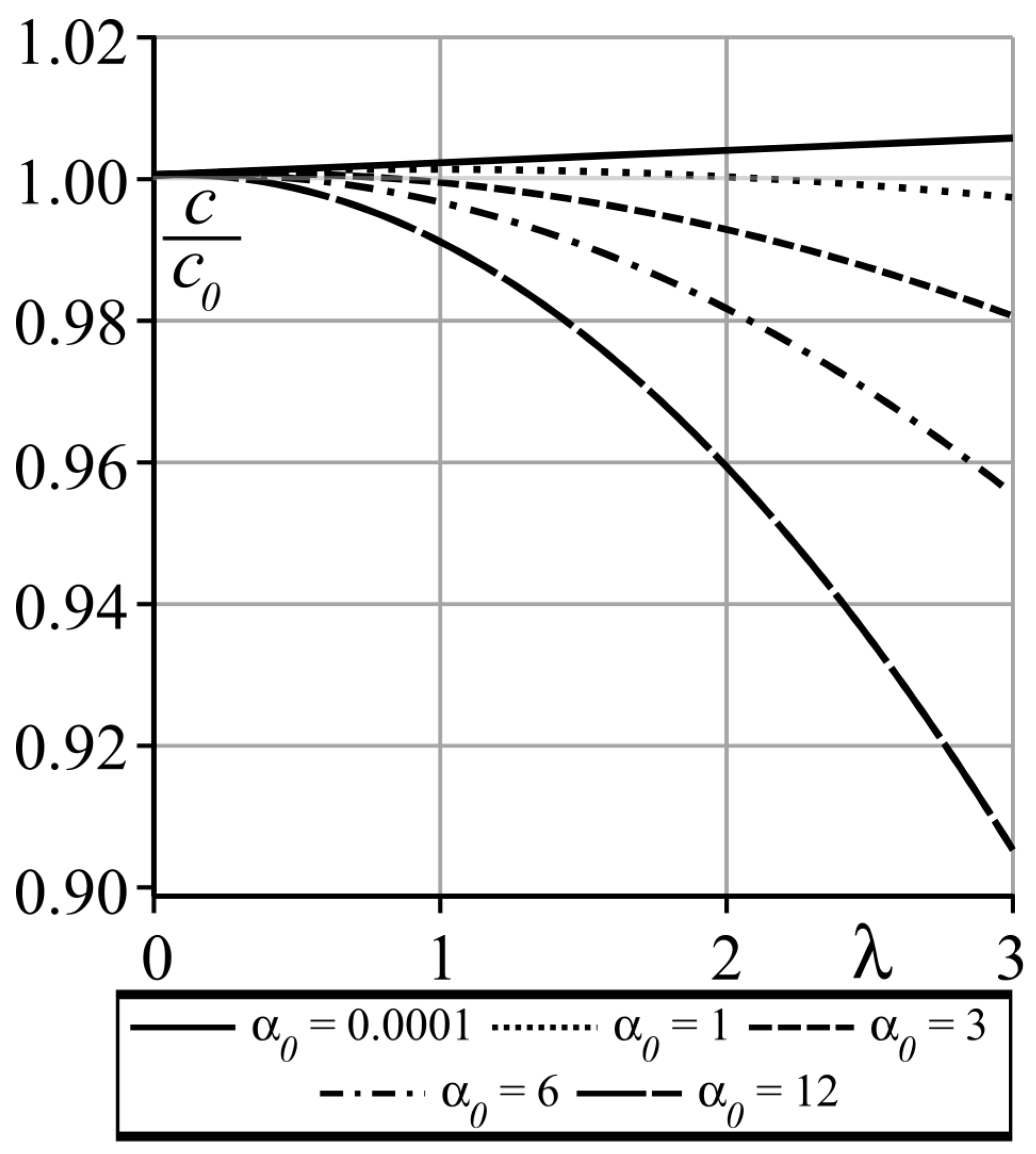
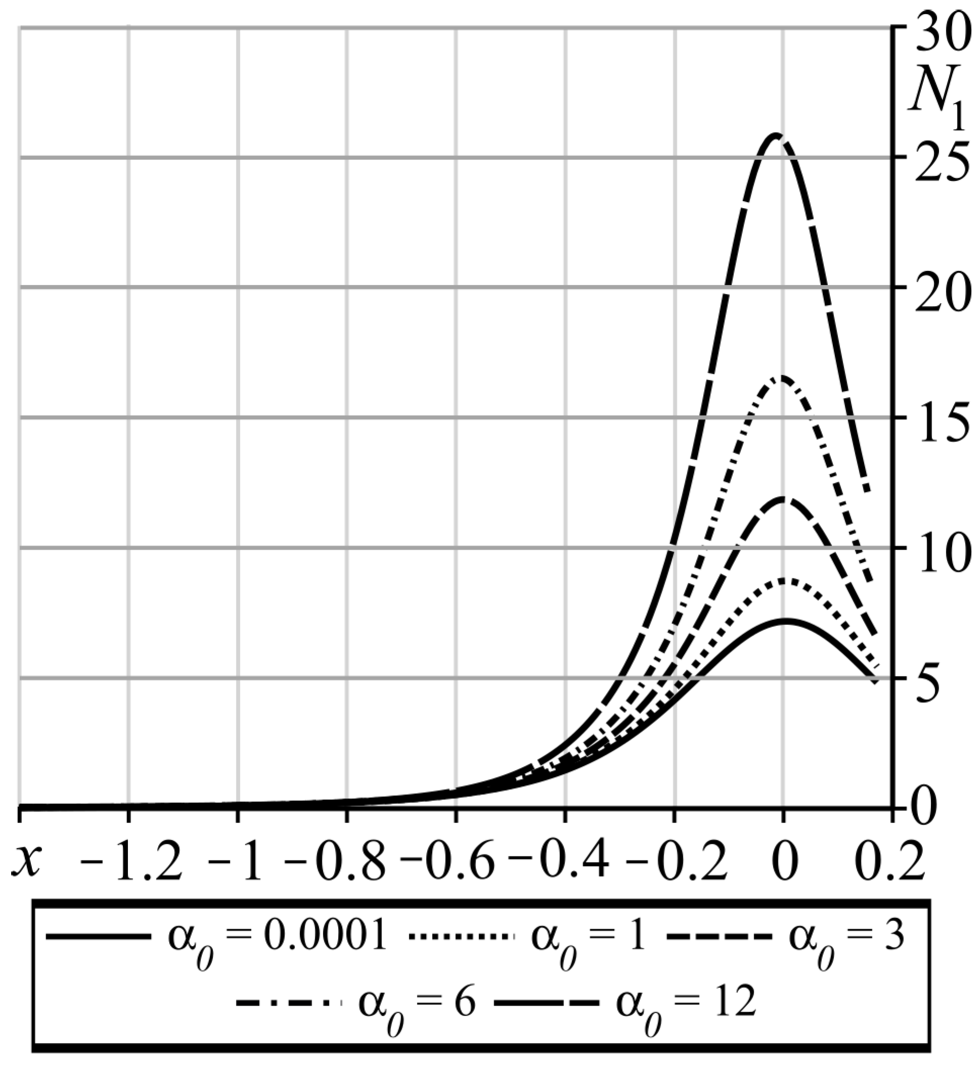
Figure 2 represents the plots of contact pressure in the lubricated contact obtained for different values of ${\alpha }_0$ and $\lambda$. For ${\alpha }_0=1$ and $\lambda =2$, the pressure distribution is very close to the one for the corresponding Newtonian fluid (see [13,29]). It is clear from these graphs that the maximum of the contact pressure tends to increase with the growth in ${\alpha }_0$ and $\lambda$, while the size of the contact region tends to decrease due to decrease in c (see Figure 3). The variations in the contact pressure distribution compared to the corresponding Newtonian one remain insignificant for small values of the mobility factor ${\alpha }_0$ even for a relatively large lubricant relaxation time $\lambda$. However, for relatively large values of the mobility factor ${\alpha }_0$, the former variations in pressure $p\left(x\right)$ and exit coordinate c become significant. 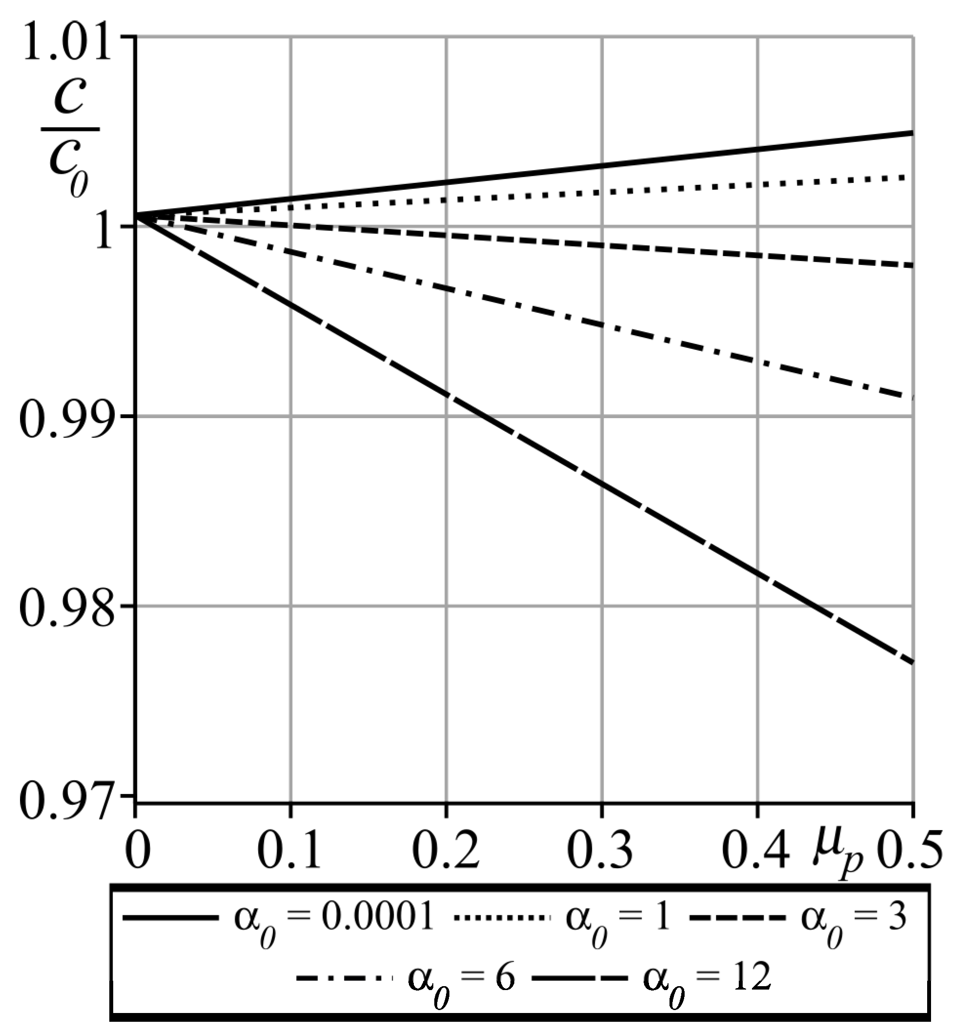Figure 4 shows the dependence of the exit coordinate c on the lubricant additive viscosity ${\mu }_p$, which qualitatively (being linear) resembles the dependence of c on $\lambda$ from Figure 3 which is nonlinear.

For ${\alpha }_0=0$, the Giesekus model becomes the convected Maxwell model and the value of the exit coordinate c tends slightly to increase with increase in both $\lambda$ and ${\mu }_p$.

The dependence of the exit film thickness $h_e$ on the lubrication relaxation time $\lambda$ and lubricant additive viscosity ${\mu }_p$ is represented in Figure 5 and Figure 6, which show beneficial (increasing) behavior of $h_e$ with increase in ${\alpha }_0,\lambda$, and ${\mu }_p$. The only difference is in whether it happens linearly or nonlinearly. A similar behavior of the minimum lubrication film thickness $h_{min}$ is shown in Figure 7 and Figure 8.

As it is clear from Figure 9 and Figure 10, depending on the value of the mobility factor ${\alpha }_0$, the friction force $F_{+}$ may display an increasing or decreasing behavior with $\lambda$ and ${\mu }_p$. Specifically, for smaller values of ${\alpha }_0$, the friction force $F_{+}$ decreases with $\lambda$ and ${\mu }_p$, while for larger values of ${\alpha }_0$, the friction force $F_{+}$ monotonically increases with $\lambda$ and ${\mu }_p$. 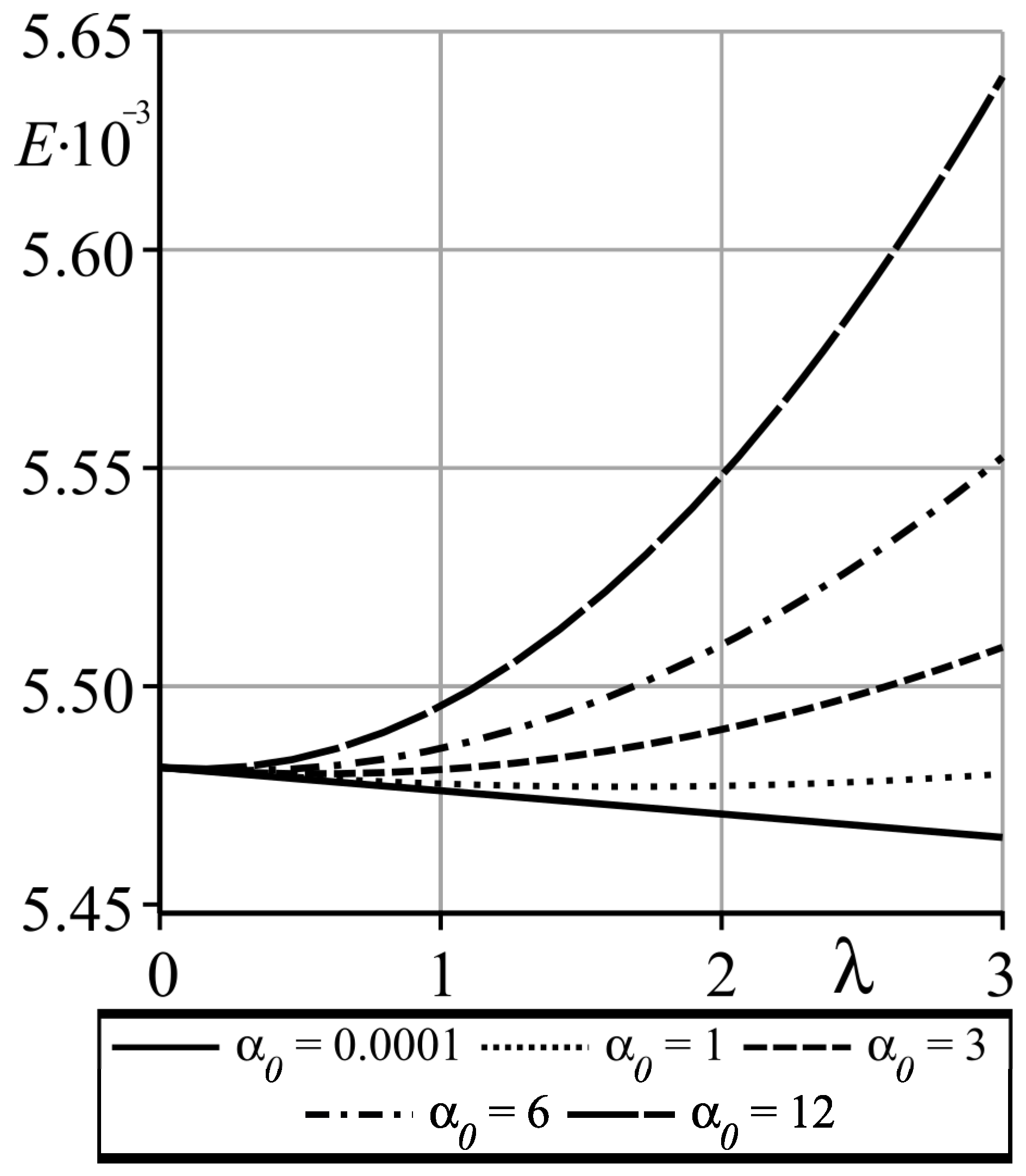A similar behavior exhibits the energy loss in the contact E presented in Figure 11. The fact that the exit lubrication film thickness $h_e$ always is greater than in the corresponding case of a Newtonian fluid and that one can pick the mobility factor ${\alpha }_0$ value for which the friction force $F_{+}$ and energy loss E are just a bit higher than in the case of a Newtonian liquid provides an opportunity to optimize the lubricant design to increase lubrication film thickness and, at the same time, to practically not increase the frictional and energy losses. For example, for ${\alpha }_0=1$ and $\lambda =3$, it is possible to achieve an increase in the minimum lubrication film thickness $h_{min}$ by about $2\%$ while the friction $F_{+}$ and energy E losses would increase by about only $1\%$ compared to the lubricant with the corresponding Newtonian rheology.

The behavior of the lubricant flux Q as a function of the lubricant relaxation time $\lambda$ and lubricant additive viscosity ${\mu }_p$ are depicted in Figure 12 and Figure 13, and its behavior resembles the behavior of the exit film thickness $h_e$ from Figure 5 and Figure 6.

Some graphs of the additional pressure distribution $N_1$ versus x for $z=0$ are presented in Figure 14 and Figure 15. In a sense, the behavior of $N_1(x,0)$ resembles the behavior of $p\left(x\right)$ from Figure 2.

7. One Problem Generalization

In the above analysis, a lubrication problem for two parallel cylinders of the same radius has been considered. Now, let us briefly consider the generalization of this problem on the case of two parallel cylinders with different radii $R_1$ and $R_2$. Then, in the same coordinate system as before, all equations of the problem formulation remain the same as before except for the boundary conditions for the lubricant velocity components, which now look as follows

$$\begin{array}{c}u(x,-H_1\left(x\right))=\overline{u_1},u(x,H_2\left(x\right))=\overline{u_2},\end{array}$$

(66)

$$\begin{array}{c}w(x,-H_1\left(x\right))=-\overline{u_1}\frac{d{H}_1\left(x\right)}{dx},w(x,H_2\left(x\right))=\overline{u_2}\frac{d{H}_2\left(x\right)}{dx},\end{array}$$

(67)

and the equilibrium condition

$$\begin{array}{c}\underset{x_i}{\overset{x_e}{\int }}[p\left(x\right)-{\tau }_{zz}(x,H_2\left(x\right))]dx=P,\end{array}$$

(68)

where $z=-H_1\left(x\right)$ and $z=H_2\left(x\right)$ are the cylinder surfaces which are represented by equations

$$\begin{array}{c}{H}_i\left(x\right)=\frac{h_e}{2}+\frac{x^2-x_e^2}{2R_i},i=1,2,h\left(x\right)=H_1\left(x\right)+H_2\left(x\right),\\ \\ H_i\left(x\right)=h_{i0}\left(x_0\right)+\alpha h_{i1}\left(x_0\right)+\dots ,i=1,2,h_e=h_{e0}+\alpha h_{e1}+\dots ,\end{array}$$

(69)

$$\begin{array}{c}{h}_0(x_0)=h_{10}(x_0)+h_{20}(x_0)=h_{e0}+\frac{x_0^2-x_{e0}^2}{2R_e},\\ \\ h_1(x_0)=h_{11}(x_0)+h_{21}(x_0)=h_{e1}+\frac{x_{e1}}{R_e}[\frac{x_0(x_0-x_i)}{x_{e0}-x_i}-x_{e0}],\end{array}$$

(70)

where $R_e$ is the effective radius of the cylinders, $1/R_e=1/R_1+1/R_2$.

The analysis of the system of these equations is conducted for $\alpha \ll 1$ in the manner similar to the one used above, but in (13), the variable z remained intact. The assumptions (11) and (23) regarding $\alpha$ and ${\lambda }_1$ remain the same. Then, using the same dimensionless variables as in (16) and asymptotic representations of solution components in which terms proportional to $h_1$ are omitted, one obtains Equations (29)–(32), in which terms proportional to $h_1$ are omitted. To derive the expressions for $u_0,w_0$, and $u_1$, one needs to use asymptotic boundary conditions (34) and (35) following from (66) and (67), in which $\frac{h_1\left(x_0\right)}{2}$ on the lower and upper surfaces should be replaced by $h_{11}\left(x_0\right)$ and $h_{21}\left(x_0\right)$, respectfully.

After that, the expressions for $u_0,w_0$, and $u_1$ have the form

$$\begin{array}{c}{u}_0(x_0,z)=\frac{(\overline{u_2}{h}_{10}+\overline{u_1}{h}_{20})}{h_0}+\frac{(\overline{u_2}-\overline{u_1})}{h_0}z+(z-h_{20})(z+h_{10})\frac{1}{2\mu }\frac{d{p}_0}{d{x}_0},\end{array}$$

(71)

$$\begin{array}{c}{w}_0(x_0,z)=-u_1\frac{d{h}_{10}}{d{x}_0}+(\overline{u_1}-\overline{u_2})\frac{{(z+h_{10})}^2}{2h_0^2}\frac{d{h}_{20}}{d{x}_0}+(\overline{u_1}-\overline{u_2})\frac{(z+h_{10})(z-h_{10}-2h_{20})}{2h_0^2}\frac{d{h}_{10}}{d{x}_0}\\ \\ +((z+h_{10})(z-h_{10}-2h_{20})\frac{d{h}_{10}}{d{x}_0}-{(z+h_{10})}^2\frac{d{h}_{20}}{d{x}_0})\frac{1}{4\mu }\frac{d{p}_0}{d{x}_0}\\ \\ +{(z+h_{10})}^2(z-h_{10}-2h_{20})\frac{1}{6\mu }\frac{d^2{p}_0}{d{x}_0^2},\end{array}$$

(72)

$$\begin{array}{lcr}& \begin{array}{c}{u}_1(x_0,z)=x_{e1}\frac{(x_0-x_i)}{(x_{e0}-x_i)}[(h_{20}-z)\frac{d{h}_{10}}{d{x}_0}+(h_{10}+z)\frac{d{h}_{20}}{d{x}_0}]\frac{1}{2\mu }\frac{d{p}_0}{d{x}_0}\\ \\ +[(z-h_{20})h_{11}-h_{21}(z+h_{10})]\frac{1}{2\mu }\frac{d{p}_0}{d{x}_0}+(u_2-u_1)x_{e1}\frac{(x_0-x_i)}{(x_{e0}-x_i)}[(z-h_{20})\frac{d{h}_{10}}{d{x}_0}\\ \\ +(h_{10}+z)\frac{d{h}_{20}}{d{x}_0}]\frac{1}{h_0^2}+(z-h_{20})(z+h_{10})\frac{1}{2\mu }\frac{d{p}_1}{d{x}_0}-(u_2-u_1)(z{h}_1+h_{12}{h}_{10}-h_{11}{h}_{20})\frac{1}{h_0^2}\\ \\ -\frac{3{\lambda }^2{\mu }_p}{{\mu }^2}\frac{d{p}_0}{d{x}_0}\{3(u_2-u_1{)}^2(z-h_{21})(z+h_{11})\frac{1}{2h_0^2}+(u_2-u_1)(z-h_{21})(z+h_{11})(z\\ \\ +\frac{h_{11}-h_{21}}{2})\frac{1}{h_0}\frac{1}{\mu }\frac{d{p}_0}{d{x}_0}+(z-h_{21})(z+h_{11})(z^2-h_{11}+h_{21}+\frac{h_{11}^2+h_{21}^2}{2})\frac{1}{4{\mu }^2}(\frac{d{p}_0}{d{x}_0}{)}^2\}\\ \\ +\frac{\lambda {\mu }_p}{2{\alpha }_0\mu }(z-h_{20})(z+h_{10})\{(u_2-u_1{)}^2\frac{1}{h_0^3}\frac{d{h}_0}{d{x}_0}+\frac{u_1+u_2}{2}\frac{1}{\mu }\frac{d^2{p}_0}{d{x}_0^2}-\frac{h_0^2}{4{\mu }^2}\frac{d{p}_0}{d{x}_0}\frac{d^2{p}_0}{d{x}_0^2}\\ \\ -\frac{h_0}{4{\mu }^2}\frac{d{h}_0}{d{x}_0}(\frac{d{p}_0}{d{x}_0}{)}^2\}+\frac{R{e}_0}{{\alpha }_0\mu }(z-h_{20})(z+h_{10})\{-(u_2-u_1)\frac{1}{24h_0^3}[(u_2-u_1)[3h_{10}^2\\ \\ +3(z+h_{20})h_{10}+z^2+h_{20}z+h_{20}^2]+4u_1{h}_0(z+2h_{10}+h_{20})]\frac{d{h}_0}{d{x}_0}\\ \\ +[-(z+2h_{10}+h_{20})\frac{h_0{u}_1}{3}+\frac{1}{4}(u_1-\frac{u_2}{3})[3h_{10}^2+3(z+h_{20})h_{10}+z^2+z{h}_{20}+h_{20}^2]\\ \\ -(u_1-u_2)(2h_{10}^2+2(z+h_{20})h_{10}+z^2+h_{20}^2)(z+2h_{10}+h_{20})\frac{1}{15h_0}]\frac{1}{4\mu }\frac{d^2{p}_0}{d{x}_0^2}\\ \\ -u_1(z+2h_{10}+h_{20})\frac{1}{12\mu }\frac{d{h}_0}{d{x}_0}\frac{d{p}_0}{d{x}_0}+[4z^4+4(5h_{10}+h_{20}-3h_0)z^3+(40h_{10}^2\\ \\ +4(5h_{20}-12h_0)h_{10}+4h_{20}^2-12h_{20}{h}_0+15h_0^2)z^2\\ \\ +(40h_{10}^3+8(5h_{20}-9h_0)h_{10}^2+(45h_0^2-48h_{20}{h}_0+20h_{20}^2)h_{10}+4h_{20}^3-12h_{20}^2{h}_0\\ \\ +15h_0^2{h}_{20})z+20h_{10}^4+8(-6h_0+5h_{20})h_{10}^3+(45h_0^2-72h_{20}{h}_0+40h_{20}^2)h_{10}^2\\ \\ +(45h_0^2{h}_{20}-48h_{20}^2{h}_0+20h_{20}^3)h_{10}+4h_{20}^4-12h_{20}^3{h}_0+15h_{20}^2{h}_0^2]\frac{1}{1440{\mu }^2}\frac{d{p}_0}{d{x}_0}\frac{d^2{p}_0}{d{x}_0^2}\\ \\ +[3h_{10}^2+3(z+h_{20})h_{10}+z^2+h_{20}z+h_{20}^2]\frac{h_0}{96{\mu }^2}\frac{d{h}_0}{d{x}_0}(\frac{d{p}_0}{d{x}_0}{)}^2\}.\end{array}& \end{array}$$

(73)

The Reynolds equations of the first and second order are derived from the equation (for comparison, see (41))

$$\begin{array}{c}\frac{d}{dx}\underset{-H_1}{\overset{H_2}{\int }}u(x,z)dz=0.\end{array}$$

(74)

Using the obtained asymptotic solution representations, one derives the zero-order Reynolds equation

$$\begin{array}{c}\frac{d}{d{x}_0}\underset{-h_{10}}{\overset{h_{20}}{\int }}{u}_0(x_0,z)dz=0,\end{array}$$

(75)

and the first-order Reynolds equation

$$\begin{array}{c}\frac{d}{d{x}_0}\{\underset{-h_{10}}{\overset{h_{20}}{\int }}{u}_{1*}(x_0,z)dz+h_{11}\overline{u_1}+h_{21}\overline{u_2}\}=0.\end{array}$$

(76)

Substitution of the expressions for $u_0$ and $u_1$ from (71) and (73) into (75) and (76) leads to precisely the same Reynolds Equations (44) and (45) with boundaries (46) and (47) and additional conditions (49) and (50) derived for the case of cylinders of the same radius R; however, in this case, $1/R_e=1/R_1+1/R_2$. The rest of the analysis is identical with the one conducted above for the case of cylinders of the same radius R.

Formulas for the friction forces $F_{fr\pm }$ and energy loss E obviously become transformed to the following ones

$$\begin{array}{c}{F}_{fr-}=\underset{x_i}{\overset{x_e}{\int }}{\tau }_{xz}(x,-H_1\left(x\right))dx,\\ \\ F_{fr+}=\underset{x_i}{\overset{x_e}{\int }}{\tau }_{xz}(x,H_2\left(x\right))dx,\\ \\ E=\underset{x_i}{\overset{x_e}{\int }}dx\underset{-H_1}{\overset{H_2}{\int }}{\tau }_{xz}(x,z)\frac{\partial u(x,z)}{\partial z}dz.\end{array}$$

(77)

8. Conclusions

This study is concerned with the new asymptotic solution of the steady hydrodynamic problem of lubrication of two rigid cylinders rolling and sliding over each other and then being separated from each other by a non-Newtonian fluid described by the Geisekus rheology. The problem is considered in the case when the lubricant mobility factor $\alpha$, lubricant relaxation time ${\lambda }_1$, and characteristic dimensionless gap $ϵ$ are of the same order of magnitude. Using the modification of the regular perturbation method, it was possible to simplify the original rheological equation of the Giesekus model and to obtain the first two Reynolds equations for determining the main and first terms of the asymptotic expansion of contact pressure with respect to small mobility factor $\alpha$. The solutions of these equations are obtained analytically. Using these solutions, the coordinate of the exit point from the contact and the exit lubrication film thickness were determined. After that, it was numerically investigated the influence of the problem input parameters on contact pressure, lubrication film thickness, lubricant flux, friction force, contact energy loss, etc. For $\alpha =0$, the Giesekus rheology turns into the convected Maxwell one. Graphs show that as the mobility factor $\alpha$ increases, the problem characteristics significantly deviate from the ones for the convected Maxwell case. Also, the solution demonstrates a significant dependence on the lubricant relaxation time. Therefore, the conclusion can be drawn that neglecting to take into account the lubricant mobility factor and lubricant relaxation time can lead to a significantly distorted picture of what is going on in a lubricated contact. The relatively simple solution obtained in the study would allow us to take into account the details of a complex rheology of lubricating oils.

References

1. Chapkov, A.D.; Bair, S.; Cann, P.; Lubrecht, A.A. Film Thickness in Point Contacts under Generalized Newtonian EHL Conditions: Numerical and Experimental Analysis. Tribol. Int. 2007, 40, 1474–1478. [Google Scholar] [CrossRef]
2. Yang, P.; Cui, J.; Jin, Z.M.; Dowson, D. Transient Elastohydrodynamic Analysis of Elliptical Contacts. Part 2: Thermal and Newtonian Lubricant Solution. Proc. Inst. Mech. Eng. Part J J. Eng. Tribol. 2005, 219, 187–200. [Google Scholar] [CrossRef]
3. Li, B.; Sun, J.; Zhu, S.; Fu, Y.; Zhao, X.; Wang, H.; Teng, Q.; Ren, Y.; Li, Y.; Zhu, G. Thermohydrodynamic Lubrication Analysis of Misaligned Journal Bearing Considering the Axial Movement of Journal. Tribol. Int. 2019, 135, 397–407. [Google Scholar] [CrossRef]
4. Wang, Z.; Hu, Y.; Wang, W.; Wang, H. Numerical Analysis of Point Contact EHL on Coated Substrates. In Proceedings of the ASME/STLE 2009 International Joint Tribology Conference, Memphis, TN, USA, 19–21 October 2009; ASMEDC: Memphis, TN, USA, 2009; pp. 471–473. [Google Scholar] [CrossRef]
5. Su, J.; Song, H.-X.; Ke, L.-L. Elastohydrodynamic Lubrication Line Contact Based on Surface Elasticity Theory. J. Appl. Mech. 2020, 87, 081004. [Google Scholar] [CrossRef]
6. Charles, P.; Elfassi, M.; Lubrecht, A.A. Double–Newtonian Rheology in a Model Piston-Ring Cylinder-Wall Contact. Tribol. Int. 2010, 43, 1902–1907. [Google Scholar] [CrossRef]
7. Katyal, P.; Kumar, P. On the Role of Second Newtonian Viscosity in EHL Point Contacts Using Double Newtonian Shear-Thinning Model. Tribol. Int. 2014, 71, 140–148. [Google Scholar] [CrossRef]
8. D’Agostino, V.; Petrone, V.; Senatore, A. Effects of the Lubricant Piezo-Viscous Properties on EHL Line and Point Contact Problems. Tribol. Lett. 2013, 49, 385–396. [Google Scholar] [CrossRef]
9. Kazama, T. A Comparative Newtonian and Thermal EHL Analysis Using Physical Lubricant Properties. In Tribology Series; Elsevier: Amsterdam, The Netherlands, 2002; Volume 40, pp. 435–446. [Google Scholar] [CrossRef]
10. Liu, Y.; Wang, Q.J.; Bair, S.; Vergne, P. A Quantitative Solution for the Full Shear-Thinning EHL Point Contact Problem Including Traction. In Proceedings of the ASME/STLE 2007 International Joint Tribology Conference, Parts A and B, San Diego, CA, USA, 22–24 October 2007; ASMEDC: San Diego, CA, USA, 2007; pp. 1031–1032. [Google Scholar] [CrossRef]
11. Cherizol, R.; Sain, M.; Tjong, J. Review of Non–Newtonian Mathematical Models for Rheological Characteristics of Viscoelastic Composites. Green Sustain. Chem. 2015, 5, 6–14. [Google Scholar] [CrossRef]
12. Bird, R.B.; Curtis, C.F.; Armstrong, R.C.; Hassager, O. Dynamics of Polymeric Liquids. In Fluid Mechanics, 2nd ed.; John Wiley & Sons: New York, NY, USA, 1987; Volume 1. [Google Scholar]
13. Kudish, I.I.; Covitch, M.J. Introduction to Modeling and Analytical Methods in Tribology; Chapman & Hall/CRC: Boca Raton, FL, USA, 2010. [Google Scholar]
14. Ree, T.; Eyring, H. Theory of Non–Newtonian Flow. I. Solid Plast. System. J. Appl. Phys. 1955, 26, 793–800. [Google Scholar] [CrossRef]
15. Cui, J.; Yang, P.; Jin, Z.M.; Dowson, D. Transient Elastohydrodynamic Analysis of Elliptical Contacts. Part 3: Non–Newtonian Lubricant Solution under Isothermal and Thermal Conditions. Proc. Inst. Mech. Eng. Part J J. Eng. Tribol. 2007, 221, 63–73. [Google Scholar] [CrossRef]
16. Su, J.; Song, H.; Ke, L.; Aizikovich, S.M. The Size-Dependent Elastohydrodynamic Lubrication Contact of a Coated Half-Plane with Non–Newtonian Fluid. Appl. Math. Mech. 2021, 42, 915–930. [Google Scholar] [CrossRef]
17. Tichy, J.A. Non–Newtonian Lubrication with the Convected Maxwell Model. J. Tribol. 1996, 118, 344–348. [Google Scholar] [CrossRef]
18. Huang, P.; Li, Z.; Meng, Y.; Wen, S. Study on Thin Film Lubrication with Second-Order Fluid. J. Tribol. 2002, 124, 547–552. [Google Scholar] [CrossRef]
19. Akyildiz, F.T.; Bellout, H. Viscoelastic Lubrication with Phan-Thein-Tanner Fluid (PTT). J. Tribol. 2004, 126, 288–291. [Google Scholar] [CrossRef]
20. Gwynllyw, D.R.; Phillips, T.N. The Influence of Oldroyd-B and PTT Lubricants on Moving Journal Bearing Systems. J. Non–Newton. Fluid Mech. 2008, 150, 196–210. [Google Scholar] [CrossRef]
21. Covitch, M.J.; Trickett, K.J. How Polymers Behave as Viscosity Index Improvers in Lubricating Oils. Adv. Chem. Eng. Sci. 2015, 5, 134–151. [Google Scholar] [CrossRef]
22. Sawyer, W.G.; Tichy, J.A. Non–Newtonian Lubrication with the Second-Order Fluid. J. Tribol. 1998, 120, 622–628. [Google Scholar] [CrossRef]
23. Taylor, R.; De Kraker, B. Shear Rates in Engines and Implications for Lubricant Design. Proc. Inst. Mech. Eng. Part J J. Eng. Tribol. 2017, 231, 1106–1116. [Google Scholar] [CrossRef]
24. Giesekus, H. A Simple Constitutive Equation for Polymer Fluids Based on the Concept of Deformation-Dependent Tensorial Mobility. J. Non–Newton. Fluid Mech. 1982, 11, 69–109. [Google Scholar] [CrossRef]
25. Giesekus, H. A Unified Approach to a Variety of Constitutive Models for Polymer Fluids Based on the Concept of Configuration-Dependent Molecular Mobility. Rheol. Acta 1982, 21, 366–375. [Google Scholar] [CrossRef]
26. Yoo, J.Y.; Choi, H.C. On the Steady Simple Shear Flows of the One-Mode Giesekus Fluid. Rheol. Acta 1989, 28, 13–24. [Google Scholar] [CrossRef]
27. Raisi, A.; Mirzazadeh, M.; Dehnavi, A.S.; Rashidi, F. An Approximate Solution for the Couette-Poiseuille Flow of the Giesekus Model between Parallel Plates. Rheol. Acta 2008, 47, 75–80. [Google Scholar] [CrossRef]
28. Abbaspur, A.; Norouzi, M.; Akbarzadeh, P.; Vaziri, S.A. Analysis of Nonlinear Viscoelastic Lubrication Using Giesekus Constitutive Equation. Proc. Inst. Mech. Eng. Part J J. Eng. Tribol. 2021, 235, 1124–1138. [Google Scholar] [CrossRef]
29. Kudish, I.I.; Volkov, S.S.; Aizikovich, S.M.; Ke, L. One simple case of lubricated line contact for double-layered elastic solids. Probl. Strength Plast. 2022, 84, 5–14. [Google Scholar] [CrossRef]
30. Kudish, I.I.; Pashkovski, E.; Volkov, S.S.; Vasiliev, A.S.; Aizikovich, S.M. Heavily Loaded Line EHL Contacts with Thin Adsorbed Soft Layers. Math. Mech. Solids 2020, 25, 1011–1037. [Google Scholar] [CrossRef]
31. Kudish, I.I.; Volkov, S.S.; Vasiliev, A.S. Lightly Loaded Hydrodynamic Thrust Bearing Lubricated by a Non–Newtonian Fluid. Adv. Struct. Mater. 2023, 170, 433–448. [Google Scholar] [CrossRef]
32. Kudish, I.; Pashkovski, E.; Patterson, R. Line Contact Lubricated by a Fluid Described by Non–Newtonian Giesekus Model. IMA J. Appl. Math. 2022, 87, 722–756. [Google Scholar] [CrossRef]
33. Van-Dyke, M. Perturbation Methods in Fluid Mechanics; Academic Press: New York, NY, USA; London, UK, 1964. [Google Scholar]
34. Kaplunov, J.D.; Nolde, E.V.; Shorr, B.F. A Perturbation Approach for Evaluating Natural Frequencies of Moderately Thick Elliptic Plates. J. Sound Vib. 2005, 281, 905–919. [Google Scholar] [CrossRef]
Figure 1. The general view of a lubricated contact.
Mathematics 11 04679 g001
Figure 2. Plots of contact pressure distributions p ( x ) for the basic set of input parameters and different values of α 0 and λ .
Mathematics 11 04679 g002
Figure 3. Plots of the dependence of the relative lubricated contact exit coordinate c / c 0 versus λ for different values of α 0 .
Mathematics 11 04679 g003
Figure 4. Plots of the dependence of the relative lubricated contact exit coordinate c / c 0 versus μ p for different values of α 0 .
Mathematics 11 04679 g004
Figure 5. Plots of the dependence of the exit lubrication film thickness h e versus λ for different values of α 0 .
Mathematics 11 04679 g005
Figure 6. Plots of the dependence of the exit lubrication film thickness h e versus μ p for different values of α 0 .
Mathematics 11 04679 g006
Figure 7. Plots of the dependence of the minimum lubrication film thickness h m i n versus λ for different values of α 0 .
Mathematics 11 04679 g007
Figure 8. Plots of the dependence of the minimum lubrication film thickness h m i n versus μ p for different values of α 0 .
Mathematics 11 04679 g008
Figure 9. Plots of the friction force F + versus λ for different values of α 0 .
Mathematics 11 04679 g009
Figure 10. Plots of the friction force F + versus μ p for different values of α 0 .
Mathematics 11 04679 g010
Figure 11. Plots of the contact energy loss E versus λ for different values of α 0 .
Mathematics 11 04679 g011
Figure 12. Plots of the lubricant volume flux Q versus λ for different values of α 0 .
Mathematics 11 04679 g012
Figure 13. Plots of the lubricant volume flux Q versus μ p for different values of α 0 .
Mathematics 11 04679 g013
Figure 14. The plots N 1 is constructed at z = 0 and λ = 1 for different values of α 0 .
Mathematics 11 04679 g014
Figure 15. The plots N 1 is constructed at z = 0 and λ = 3 for different values of α 0 .
Mathematics 11 04679 g015
Disclaimer/Publisher’s Note: The statements, opinions and data contained in all publications are solely those of the individual author(s) and contributor(s) and not of MDPI and/or the editor(s). MDPI and/or the editor(s) disclaim responsibility for any injury to people or property resulting from any ideas, methods, instructions or products referred to in the content.