Stationary Pattern and Global Bifurcation for a Predator–Prey Model with Prey-Taxis and General Class of Functional Responses

Abstract

This paper will explore a predator–prey model that incorporates prey-taxis and a general functional response in a bounded domain. Firstly, we will examine the stability and pattern formation of both local and nonlocal models. Our main finding is that the inclusion of nonlocal terms enhances linear stability, and the system can generate patterns due to the effects of prey-taxis. Secondly, we consider the nonlinear prey-taxis as the bifurcation parameter in order to analyze the global bifurcation of this model. Specifically, we identify a branch of nonconstant solutions that emerges from the positive constant solution when the prey-tactic sensitivity is repulsive. Finally, we will validate the effectiveness of the theoretical conclusions using numerical simulation methods.

1. Introduction

In population ecology, the key research field of ecological systems is the spatial and temporal behaviors of interacting species. Based on this, numerous variations of predator–prey models has been proposed and extensively investigated within this research domain. Motivated by previous work [1,2,3,4], it is found that the predator–prey interaction can be illustrated as the rate of feeding upon prey for predator, which can be termed as the functional response of predator. One of the most extensively studied applications of the prey-taxis model is in the field of ecology, where it has been used to understand predator–prey dynamics. Therefore, the model has been used to examine the behavior of predators and their impact on prey populations. For instance, researchers have used the model to study how predators select their prey, how they use cues to locate prey, and how they affect the distribution of prey populations [5,6]. Therefore, this paper is dedicated to examining a highly interconnected prey-taxis model with a wide range of general functional responses.

$$\left\{\begin{array}{cc}{u}_t=d_u\Delta u-\nabla (u\chi \nabla v)+u(c\mathcal{ϝ}\left(v\right)-b),\hfill & \mathrm{in}\mathrm{\Omega }\times (0,T),\hfill \\ v_t=d_v\Delta v+rv(1-\frac{v}{k})-u\mathcal{ϝ}\left(v\right),\hfill & \mathrm{in}\mathrm{\Omega }\times (0,T),\hfill \\ \frac{\partial u}{\partial \nu }=\frac{\partial v}{\partial \nu }=0,\hfill & \mathrm{on}\partial \mathrm{\Omega },\hfill \\ u(0,x)=u_0\left(x\right),v(0,x)=v_0\left(x\right),\hfill & \mathrm{in}\mathrm{\Omega }.\hfill \end{array}\right.$$

(1)

In this model, $\mathrm{\Omega }$ is a bounded domain in $R^N$ ($N\ge 1$ is an integer) with a smooth boundary $\partial \mathrm{\Omega }$; u and v present the densities of the predator and prey, respectively; $d_u$ and $d_v$ are positive constants; and $\chi$ is an arbitrary constant. $\Delta$ is laplace operator, which represents the random movement of species; the term $-\nabla (u\chi \nabla v)$ gives the velocity by which predators move up the gradient of prey; and prey-taxis is commonly referred to attractive (repulsive) if $\chi >0$$(\chi <0)$. b means the per capita death rate of predators; $rv(1-\frac{v}{k})$ is the logistical growth rate of prey; and r and k show the prey’s intrinsic growth rate and the carrying capacity of the prey, respectively. $\nu$ denotes the outward normal vector field on $\partial \mathrm{\Omega }$; it is a closed system. Reaction–diffusion models incorporating strictly prey-dependent functional responses play a crucial role in comprehending the dynamics of predator–prey interactions and have applications in various fields, including ecology, population biology, and conservation biology. Commonly, the used functional responses are as follows:

• Holling Type I [1,4,7]: $\mathcal{ϝ}\left(v\right)=v$;
• Holling Type II [1,4,8,9]: $\mathcal{ϝ}\left(v\right)=\frac{v}{a+v}$;
• Holling Type III [1,4,9,10]: $\mathcal{ϝ}\left(v\right)=\frac{v^{\varrho }}{a^{\varrho }+v^{\varrho }}$;
• Holling Type IV [11,12,13,14]: $\mathcal{ϝ}\left(v\right)=\frac{v}{a+v^2}$;
• Other types of response functions can be found in [15,16,17,18,19,20].

Here, $a,b,c$ are all positive constants and $\varrho >1$.

Henceforth, we assume that

$$\left(H\right)\mathcal{ϝ}\left(v\right)\ge 0\mathrm{for}\mathrm{all}v\in [0,\infty ),\mathrm{and}{\mathcal{ϝ}}_v\left(v\right)\ge 0\mathrm{for}\mathrm{all}v\in [0,\infty ).$$

Many researchers have already investigated the existence of periodic solutions and the equilibrium point by using the theoretical method of ordinary differential equations (see [1,6,11,12,13,14]). However, the dynamic structure of a reaction–diffusion model is not solely influenced by the functional response, but also depends on various other factors, such as maturity delay [1,4], spatial diffusion [2,15], and location [7,10,15,21,22]. Indeed, in addition to these factors, in ecological models, the inclusion of a prey-taxis term is inevitable, which indicates that the movement or velocity of predators is influenced by the spatial and temporal distribution of their prey. Moreover, this term implies that predators tend to move toward areas with higher prey density or where the prey density is increasing. Researchers aim to enhance the accuracy of capturing predator–prey interactions and simulate the dynamics of these populations in a spatially explicit manner by incorporating the prey-taxis term into models. This mechanism depicts how predators adapt their behavior based on the availability and movement of their prey. Therefore, many researchers have investigated spatial predator–prey systems incorporating prey-taxis and have recognized that these systems exhibit more diverse dynamics and generate different spatial patterns compared to systems without prey-taxis. These dynamics can include chaotic solutions and solutions that become quasi-periodic as the values of prey-taxis change [8,23,24]. For example, in [1], the authors conducted a study on System (1) and utilized the Schauder fixed-point theorem and duality technique to demonstrate the existence and uniqueness of weak solutions in their work [1]. Thereafter, Wang et al. [14] studied the global bifurcation of System (1) by adding Holling Type II functional response. They proved that a branch of nonconstant solutions can bifurcate from the positive equilibrium only when the chemotactic is repulsive. Furthermore, they obtained stable bifurcating solutions near the bifurcation point under suitable conditions. In a related work, Luo and Wang [3] obtained the global bifurcation structure of nonconstant steady states for a reaction–diffusion predator–prey model with prey-taxis and double Beddington-DeAngelis functional responses. Motivated by the aforementioned papers [14,21], we refer to [1,6,11,14,15,21] for a background on ordinary differential models and to [8,16,17,23,25] for diffusive models.

Researchers have extensively studied nonlocal competition effects in reaction–diffusion systems due to the recognition that prey not only interacts locally with other prey or predators in the same location, but also in different locations, potentially even across the entire space. The inclusion of nonlocal interaction terms into the reaction kinetics is necessary to capture these dynamics accurately [26,27,28]. In previous work [26], the most straightforward approach to incorporate nonlocal effects is to replace the term $\frac{v}{k}$, which represents the intraspecific competition of the prey population, with $\frac{\overline{v}}{k}$ in the predator–prey system, where

$$\overline{v}={\int }_{\mathrm{\Omega }}G(x,y)v(y,t)dy,$$

where $G(x,y)$ is some reasonable kernel and $\mathrm{\Omega }$ is the spatial domain. These previous works [27,28] motivate us to introduce the nonlocal intraspecific competition into System (1), and the kernel function $G(x,y)$ takes the simplest case $G(x,y)=1/Vol\left(\mathrm{\Omega }\right)$. In this paper, we consider the following system

$$\left\{\begin{array}{cc}{u}_t=d_u\Delta u-\nabla (u\chi \nabla v)+u(c\mathcal{ϝ}\left(v\right)-b),\hfill & \mathrm{in}\mathrm{\Omega }\times (0,T),\hfill \\ v_t=d_v\Delta v+rv(1-\frac{{\int }_{\mathrm{\Omega }}vdx}{kVol\left(\mathrm{\Omega }\right)})-u\mathcal{ϝ}\left(v\right),\hfill & \mathrm{in}\mathrm{\Omega }\times (0,T),\hfill \\ \frac{\partial u}{\partial \nu }=\frac{\partial v}{\partial \nu }=0,\hfill & \mathrm{on}\partial \mathrm{\Omega },\hfill \\ u(0,x)=u_0\left(x\right),v(0,x)=v_0\left(x\right),\hfill & \mathrm{in}\mathrm{\Omega }.\hfill \end{array}\right.$$

(2)

The organization of this paper is as follows. In Section 2, we study the stability and pattern formation of positive constant steady states of the general models (1) and (2). In Section 3, firstly, we give a priori estimates of steady states of special predator–prey Model (1). Secondly, we employ abstract global bifurcation theory to demonstrate the existence of nonconstant positive steady states, which bifurcate from the positive constant solution. This finding suggests that pattern formation can occur only when the prey-taxis is repulsive ($\chi <0$). In Section 4, we provide numerical simulations of Model (1) with a Holling Type IV functional response. Finally, some conclusions and discussions are presented in Section 5.

2. Stability and Pattern Formation

In this section, we examine the stability of positive constant solutions of System (1). The stability of the predator–prey model depends on the parameters of the system, such as the predation rate and the growth rate of prey. By analyzing the eigenvalues of the Jacobian matrix, which describes the linearized dynamics of the model, one can determine the stability properties of the equilibrium points. Pattern formation in the predator–prey model can lead to interesting phenomena, such as the formation of predator “hotspots” or prey aggregations. These patterns can have important ecological implications, influencing the distribution and abundance of species in an ecosystem. Throughout this paper, we denote

$$f(u,v)=u(c\mathcal{ϝ}\left(v\right)-b),g(u,v)=rv(1-\frac{v}{k})-u\mathcal{ϝ}\left(v\right).$$

By [9], this constant steady-state solution is linear unstable if it satisfies Conditions (a) and (b), where

(a) The solution is stable as an equilibrium of the ordinary differential system

$$\frac{\partial u}{\partial t}=f(u,v),\frac{\partial v}{\partial t}=g(u,v).$$

(3)

(b) The solution is unstable as an equilibrium of the spatiotemporal system (1).

First, we assume that System (3) admits an internal equilibrium point denoted by $(u_1,v_1)$, i.e., $F\left(v_1\right)=b/c,u_1=\frac{rc{v}_1(1-v_1/k)}{b}$, and we study the linear stability of the ordinary differential system in the neighborhood of equilibrium $(u_1,v_1)$. The Jacobian matrix of (3) evaluated at the equilibrium points $(u_1,v_1)$ is

$$\begin{array}{cc}\hfill J& :=\left(\begin{array}{cc}{f}_u& f_v\\ g_u& g_v\end{array}\right),\hfill \end{array}$$

(4)

where

$$f_u=f_u(u_1,v_1)=c\mathcal{ϝ}\left(v_1\right)-b=0,f_v=f_v(u_1,v_1)=c{u}_1{\mathcal{ϝ}}_v\left(v_1\right),$$

(5)

$$g_u=g_u(u_1,v_1)=-\mathcal{ϝ}\left(v_1\right),g_v=g_v(u_1,v_1)=\frac{r(k-2v_1)}{k}-u_1{\mathcal{ϝ}}_v\left(v_1\right).$$

(6)

The characteristic equation of J is

$${\eta }^2-tr\left(J\right)\eta +det\left(J\right)=0,$$

(7)

where

$$tr\left(J\right)=f_u+g_v=\frac{r(k-2v_1)}{k}-u_1{\mathcal{ϝ}}_v\left(v_1\right),$$

(8)

$$det\left(J\right)=f_u{g}_v-f_v{g}_u=c{u}_1\mathcal{ϝ}\left(v_1\right){\mathcal{ϝ}}_v\left(v_1\right).$$

(9)

Next, it follows from $\left(H\right)$, we obtain if

$$\mathcal{ϝ}\left(v_1\right)>0\mathrm{and}{\mathcal{ϝ}}_v\left(v_1\right)>\max \{0,\frac{1}{u_1}(r-\frac{2r{v}_1}{k})\}$$

hold, then the equilibrium $(u_1,v_1)$ is stable for the ordinary differential system.

2.1. Linear Stability Analysis of the Local System (1)

Define a real-valued Hilbert space

$$\mathcal{X}:=\{{(u,v)}^T\in H^2\left(\mathrm{\Omega }\right)\times H^2\left(\mathrm{\Omega }\right):\frac{\partial u}{\partial \nu }=\frac{\partial v}{\partial \nu }=0atx\in \partial \mathrm{\Omega }\}$$

with the inner product defined by

$$⟨{\tilde{U}}_1,{\tilde{U}}_2⟩:={\int }_{\mathrm{\Omega }}\left(\widetilde{U_1}{\widetilde{U_2}}^T\right)dx,$$

where ${\tilde{U}}_1={({\tilde{u}}_1,{\tilde{v}}_1)}^T\in \mathcal{X}$ and ${\tilde{U}}_2={({\tilde{u}}_2,{\tilde{v}}_2)}^T\in \mathcal{X}$. We call $\tilde{u}$ and $\tilde{v}$ a small perturbation of the steady state and substitute

$$\left\{\begin{array}{c}u=u_1+\tilde{u}\hfill \\ v=v_1+\tilde{v}\hfill \end{array}\right.$$

into System (1) and omitting the higher-order terms. We linearize the local Model (1) at equilibrium point $(u_1,v_1)$ to obtain the following linearized system

$${\mathrm{\Psi }}_t=D{\mathrm{\Psi }}_{xx}+J\mathrm{\Psi },$$

(10)

with

$$\mathrm{\Psi }=\left(\begin{array}{c}\tilde{u}\\ \tilde{v}\end{array}\right),D=\left(\begin{array}{cc}{d}_u& -\chi u_1\\ 0& d_v\end{array}\right),J=\left(\begin{array}{cc}0& f_v\\ g_u& g_v\end{array}\right),$$

where $f_v,g_u$, and $g_v$ are given by Equations (5) and (6).

By simple calculation, we can solve the linear System (10) and obtain

$$\mathrm{\Psi }(x,t)={\displaystyle \sum _{n=0}^{\infty }}{p}_n{e}^{\eta t}{\mathrm{\Phi }}_n\left(x\right),n\in \mathbb{N}:=\{0,1,2,3,\dots \},$$

whose components can be found by performing a Fourier expansion of the initial conditions, where $p_n={({\rho }_n,{\varrho }_n)}^T$ is a constant vector, and ${\mathrm{\Phi }}_n\left(x\right)$ are eigenfunctions of the laplace operator

$$\left\{\begin{array}{cc}\Delta u+{\mu }_{n}u=0,\hfill & in\mathrm{\Omega },\hfill \\ \frac{\partial u}{\partial \nu }=0,\hfill & on\partial \mathrm{\Omega }.\hfill \end{array}\right.$$

(11)

Hence, we obtain eigenvalues ${\mu }_n\ge 0$ with corresponding eigenfunctions ${\mathrm{\Phi }}_n\left(x\right)$.

Substitute $p_n{e}^{\eta t}{\mathrm{\Phi }}_n\left(x\right)$ into (10). Then,

$$(\eta I-L({\mu }_n,\chi ))p_n=0.$$

Here,

$$L({\mu }_n,\chi )=\left(\begin{array}{cc}-d_u{\mu }_n& \chi u_1{\mu }_n+f_v\\ g_u& -d_v{\mu }_n+g_v\end{array}\right)$$

and I is an identity matrix. As a consequence, $\eta$ is an eigenvalue of L, and the corresponding eigenvalue equation is

$${\eta }^2-P({\mu }_n,\chi )\eta +Q({\mu }_n,\chi )=0,$$

(12)

where

$$P({\mu }_n,\chi )=-(d_u+d_v){\mu }_n+g_v,Q({\mu }_n,\chi )=d_u{d}_v{\mu }_n^2-(d_u{g}_v+\chi u_1{g}_u){\mu }_n-f_v{g}_u.$$

(13)

Suppose that $(u_1,v_1)$ is linear stable with respect to the ordinary differential model (i.e., $\mathcal{ϝ}\left(v_1\right)>0$ and ${\mathcal{ϝ}}_v\left(v_1\right)>\max \{0,\frac{1}{u_1}(r-\frac{2r{v}_1}{k})\}$ hold), that is to say

$$P({\mu }_n,0)=-(d_u+d_v){\mu }_n+g_v<0,Q({\mu }_n,0)=d_u{d}_v{\mu }_n^2-d_u{g}_v{\mu }_n-f_v{g}_u>0.$$

(14)

Hence, we can deduce that the characteristic roots of (12) have negative real parts. The following results can be directly obtained.

Theorem 1.

If $\mathcal{ϝ}\left(v_1\right)>0$ and ${\mathcal{ϝ}}_v\left(v_1\right)>\max \{0,\frac{1}{u_1}(r-\frac{2r{v}_1}{k})\}$ hold, then $(u_1,v_1)$ is locally stable for Model (1) without prey-taxis $(\chi =0)$. That is, diffusion-driven instability will not occur in System (1).

We wonder whether prey-taxis drive the instability of $(u_1,v_1)$ to occur for some values of the parameter χ.

Theorem 2.

If $\mathcal{ϝ}\left(v_1\right)>0$ and ${\mathcal{ϝ}}_v\left(v_1\right)>\max \{0,\frac{1}{u_1}(r-\frac{2r{v}_1}{k})\}$ hold. Then, the necessary condition for the prey-taxis-driven instability of $(u_1,v_1)$ is $\chi <{\chi }^{*}$, and $(u_1,v_1)$ is locally asymptotically stable for $\chi >{\chi }^{*}$, where

$${\chi }^{*}:=\frac{2\sqrt{-d_u{d}_v{f}_v{g}_u}-d_u{g}_v}{u_1{g}_u}.$$

(15)

Proof. 

Because the ordinary differential model is stable (i.e., $\mathcal{ϝ}\left(v_1\right)>0$ and ${\mathcal{ϝ}}_v\left(v_1\right)>\max \{0,\frac{1}{u_1}(r-\frac{2r{v}_1}{k})\}$), it is easy to obtain

$$P({\mu }_n,\chi )=-(d_u+d_v){\mu }_n+g_v<0.$$

To prove prey-taxis-driven instability, we must have

$$Q({\mu }_n,\chi )=d_u{d}_v{\mu }_n^2-(d_u{g}_v+\chi u_1{g}_u){\mu }_n-f_v{g}_u<0$$

(16)

for some positive integer n. Then, a necessary condition for the instability of $(u_1,v_1)$ is

$$d_u{g}_v+\chi u_1{g}_u>0\mathrm{and}\min Q({\mu }_n,\chi )=-f_v{g}_u-\frac{{(d_u{g}_v+\chi u_1{g}_u)}^2}{4d_u{d}_v}<0,$$

which are equivalent to

$$\chi <-\frac{d_u{g}_v}{u_1{g}_u}\mathrm{and}-4d_u{d}_v{f}_v{g}_u<{(d_u{g}_v+\chi u_1{g}_u)}^2.$$

(17)

Since $\chi <-\frac{d_u{g}_v}{u_1{g}_u}$, the second inequality of (17) becomes

$$2\sqrt{-d_u{d}_v{f}_v{g}_u}<d_u{g}_v+\chi u_1{g}_u.$$

Hence, it can be observed that the necessary condition for the prey-taxis-driven instability of $(u_1,v_1)$ is

$$\chi <{\chi }^{*}:=\frac{2\sqrt{-d_u{d}_v{f}_v{g}_u}-d_u{g}_v}{u_1{g}_u}.$$

Similarly, we obtain that $(u_1,v_1)$ is asymptotically stable for

$$d_v{g}_v+\chi u_1{g}_u\le 0,$$

or

$$\min Q({\mu }_n,\chi )=-d_u{d}_v{f}_v{g}_u-\frac{{(d_u{g}_v+\chi u_1{g}_u)}^2}{4}>0.$$

Therefore, $(u_1,v_1)$ is locally asymptotically stable for $\chi >{\chi }^{*}$. □

Remark 1.

In Theorem 2, we investigate the instability of a bounded spatial domain with Neumann boundary conditions. In a bounded system, the wave number n can only take on discrete values, thus implying that the wave number n can be any positive integer. If $\chi <{\chi }^{*}$ and ${\mu }_n\in ({\mu }^{-},{\mu }^{+})$ for some $n\in N^{+}$, where ${\mu }^{-},{\mu }^{+}>0$ are the two roots of $Q({\mu }_n,\chi )=0$, then we can obtain a standard Turing space, in which the equilibrium solution $(u_1,v_1)$ is linearly unstable. Therefore, the instability condition of Theorem 2 is only necessary but not sufficient.

If we choose a finite domain $\mathrm{\Omega }=(0,l\pi )$, the following result is a direct consequence of Theorem 2. The following result is about the sufficient conditions for instability of the considered system.

Theorem 3.

For $\mathrm{\Omega }=(0,l\pi )$, suppose that $\mathcal{ϝ}\left(v_1\right)>0$ and ${\mathcal{ϝ}}_v\left(v_1\right)>\max \{0,\frac{1}{u_1}(r-\frac{2r{v}_1}{k})\}$ hold. If $\chi \ge {\chi }_c$, where

$${\chi }_c:=\frac{1}{u_1{g}_u}(\frac{d_u{d}_v}{l^2}+2\sqrt{-d_u{d}_v{f}_v{g}_u}-d_u{g}_v),$$

(18)

then $(u_1,v_1)$ is an unstable state of the prey-taxis system (1). That is, the prey-taxis-driven instability.

Proof. 

A well-known conclusion is that the following eigenvalue problem

$$-{\mathrm{\Phi }}_{xx}=\mu \mathrm{\Phi },x\in (0,l\pi ),{\mathrm{\Phi }}^{\prime }\left(0\right)={\mathrm{\Phi }}^{\prime }\left(l\pi \right)=0$$

has eigenvalues ${\mu }_n=n^2/l^2$ ($n\in \mathbb{N}$), with corresponding eigenfunctions ${\mathrm{\Phi }}_n\left(x\right)=cos\left(\frac{n}{l}x\right)$. Then, we have the matrix

$$L({\mu }_n,\chi ):=\left(\begin{array}{cc}-d_u{n}^2/l^2& \chi u_1{n}^2/l^2+f_v\\ g_u& -d_v{n}^2/l^2+g_v\end{array}\right).$$

(19)

From Theorem 2, let ${\left(n^{-}\right)}^2$ and ${\left(n^{+}\right)}^2$ be the two roots of $Q({\mu }_n,\chi )=0$ in (13). By (13), we obtain that

$$0<{\left(n^{-}\right)}^2<{\left(n^{+}\right)}^2,$$

where

$${\left(n^{\pm }\right)}^2=\frac{(d_u{g}_v+u_1\chi g_u\pm \sqrt{{(d_u{g}_v+u_1\chi g_u)}^2+4d_u{d}_u{f}_v{g}_u)})l^2}{2d_v{d}_u}.$$

(20)

Thus, in order to obtain the instability of $(u_1,v_1)$, we must have ${\left(n^{-}\right)}^2<n^2<{\left(n^{+}\right)}^2$ for some positive integer n, and a necessary condition is $n^{+}-n^{-}\ge 1$, which results in

$$\frac{(d_u{g}_v+u_1\chi g_u)l^2}{d_u{d}_v}-\frac{\sqrt{-4d_u{d}_v{f}_v{g}_u}}{d_u{d}_v}\ge 1.$$

(21)

By (21), we have

$$\chi \ge {\chi }_c.$$

□

Remark 2.

For the critical prey-taxis coefficients ${\chi }^{*}$ and ${\chi }_c$, we can easily obtain ${\displaystyle \underset{l\to \infty }{lim}}{\chi }_c={\chi }^{*},$ which means that the critical value of the necessary and sufficient conditions are the same when the feasible domain $\left(\mathrm{\Omega }\right)$ is large enough.

2.2. Linear Stability Analysis of the Nonlocal System (2)

In this subsection, we analyze the nonlocal competition model (2). Now, for convenience of statements, we define the following notations

$$\left\{\begin{array}{c}\tilde{f}(u,v)=u(c\mathcal{ϝ}\left(v\right)-b),\hfill \\ \tilde{g}(u,v)=rv(1-\frac{{\int }_{\mathrm{\Omega }}vdx}{kVol\left(\mathrm{\Omega }\right)})-u\mathcal{ϝ}\left(v\right).\hfill \end{array}\right.$$

(22)

Let

$$⟨1,v⟩\left(t\right):={\int }_{\mathrm{\Omega }}v(x,t)dx,t>0.$$

(23)

Substituting

$$\begin{array}{c}\hfill \left\{\begin{array}{c}u=u_1+\tilde{u}\hfill \\ v=v_1+\tilde{v}\hfill \end{array}\right.\end{array}$$

(24)

into System (2), and we obtain the following linearized system by omitting the higher-order terms

$${\mathrm{\Psi }}_t=D{\mathrm{\Psi }}_{xx}+J_1\mathrm{\Psi }+J_2\mathrm{\Psi },$$

(25)

with

$$J_1=\left(\begin{array}{cc}0& f_v\\ g_u& A\end{array}\right),J_2=\left(\begin{array}{cc}0& 0\\ 0& S⟨1,·⟩\end{array}\right),$$

where

$$S:=\frac{r{v}_1}{k},A:=\frac{r(k-v_1)}{k}-u_1{\mathcal{ϝ}}_v\left(v_1\right)=g_v+S,{\tilde{f}}_u=f_u,{\tilde{g}}_v=g_v,$$

$D,\mathrm{\Psi },f_v,g_u$, and $g_v$ are given by Section 2.1. Since $\tilde{g}(u,v)$ includes integrals, their differentiation requires a bit more attention. We obtain

$${\tilde{g}}_v=\frac{r(k-v_1)}{k}-u_1{\mathcal{ϝ}}_v\left(v_1\right)-\frac{r{v}_1}{k}⟨1,·⟩.$$

The linearized operator of System (25) at ($u_1,v_1$) is given by

$$L({\mu }_n,\chi )=\left(\begin{array}{cc}-d_u{\mu }_n& \chi u_1{\mu }_n+f_v\\ g_u& -d_v{\mu }_n+{\hat{g}}_v\end{array}\right),$$

where

$${\hat{g}}_v=\left\{\begin{array}{c}A-Sifn=0,\hfill \\ Aifn\ne 0.\hfill \end{array}\right.$$

Taking $n=0$, we obtain the temporal model, where the characteristic equation of the ordinary differential model is

$${\eta }^2-tr\left(J\right)\eta +det\left(J\right)=0.$$

In the spatial–temporal model $(n>0)$, we have

$${\eta }^2-P({\mu }_n,\chi )\eta +Q({\mu }_n,\chi )=0,$$

(26)

where $n\in {\mathbb{N}}^{+}:=\{1,2,3,\dots \}$ and

$$P({\mu }_n,\chi )=-(d_u+d_v){\mu }_n+A,Q({\mu }_n,\chi )=d_u{d}_v{\mu }_n^2-(d_{u}A+\chi u_1{g}_u){\mu }_n-f_v{g}_u.$$

(27)

If

$$tr\left(J\right)<0,det\left(J\right)>0,P({\mu }_n,\chi )<0\mathrm{and}Q({\mu }_n,\chi )>0\mathrm{for}\mathrm{all}n\in {\mathbb{N}}^{+},$$

then $(u_1,v_1)$ is locally stable with respect to (2).

From the proofs of Theorems 2 and 3, we can obtain the following results:

Corollary 1.

Assume that $\mathcal{ϝ}\left(v_1\right)>0$ and ${\mathcal{ϝ}}_v\left(v_1\right)>\max \{0,\frac{1}{u_1}(r-\frac{r{v}_1}{k})\}$ hold. Then, the diffusion coefficients does not affect the stability of $(u_1,v_1)$, and the necessary condition for the prey-taxis-driven instability of $(u_1,v_1)$ is $\chi <{\tilde{\chi }}^{*}$, where

$${\tilde{\chi }}^{*}:=\frac{2\sqrt{-d_u{d}_v{f}_v{g}_u}-d_{u}A}{u_1{g}_u}.$$

(28)

Corollary 2.

Assume that $\mathcal{ϝ}\left(v_1\right)>0$ and ${\mathcal{ϝ}}_v\left(v_1\right)>\max \{0,\frac{1}{u_1}(r-\frac{r{v}_1}{k})\}$ hold. Then, for the critical prey-taxis coefficients ${\chi }^{*}$ and ${\tilde{\chi }}^{*}$ in Theorem 2 and Corollary 1, we have

$${\chi }^{*}\ge {\tilde{\chi }}^{*},$$

which means that if the local model is stable, then the nonlocal model is always stable. However, if the nonlocal model is stable, it does not necessarily mean that the local model will not produce spatial patterns.

3. Global Bifurcation Analysis

In this section, our focus is on examining the steady-state solutions of Model (1). It is worth noting that, according to the proof of Theorem 1, we can observe that the diffusion coefficient does not have an impact on the steady-state solutions of (1). Therefore, for shorten notation, we suppose $d_u=d_v=1$ and consider the following elliptic systems

$$\left\{\begin{array}{cc}\Delta u-\nabla (u\chi \nabla v)+u\left(c\mathcal{ϝ}\right(v)-b)=0,\hfill & \mathrm{in}\mathrm{\Omega }\times (0,T),\hfill \\ \Delta v+rv(1-\frac{v}{k})-u\mathcal{ϝ}\left(v\right)=0,\hfill & \mathrm{in}\mathrm{\Omega }\times (0,T),\hfill \\ \frac{\partial u}{\partial \nu }=\frac{\partial v}{\partial \nu }=0\hfill & \mathrm{on}\partial \mathrm{\Omega }.\hfill \end{array}\right.$$

(29)

The study of a priori estimates of the positive solution of (29) is necessary to obtain the existence of nonconstant positive solutions of (29).

Theorem 4.

If $(u,v)$ is any non-negative solution to (29). Then, there are constants $M>0,N>0$ independent of $u,v$ such that

$${\Vert u\Vert }_{\infty }\le Mand{\Vert v\Vert }_{\infty }\le N.$$

Proof. 

Firstly, for System (29), one can apply the maximum principle to obtain $u\ge 0,v\ge 0$. Then, we consider the equations of prey in (29)

$$\left\{\begin{array}{cc}-\Delta v=rv(1-\frac{v}{k})-u\mathcal{ϝ}\left(v\right),\hfill & \mathrm{in}\mathrm{\Omega },\hfill \\ \frac{\partial v}{\partial \nu }=0,\hfill & \mathrm{on}\partial \mathrm{\Omega }.\hfill \end{array}\right.$$

Let $x_0\in \overline{\mathrm{\Omega }}$ be a point such that $v\left(x_0\right)={\displaystyle \underset{\overline{\mathrm{\Omega }}}{max}}v\left(x\right)$. Using the Maximum principle again, it is easy to obtain $0<v\left(x\right)<k$. So, we just have to prove ${\Vert u\Vert }_{\infty }\le M$.

Integrating the two equations of System (29) with $\mathrm{\Omega }$,

$${\int }_{\mathrm{\Omega }}(\Delta u-\nabla (u\chi \nabla v)+u(c\mathcal{ϝ}\left(v\right)-b))dx=0$$

$${\int }_{\mathrm{\Omega }}(\Delta v+rv(1-\frac{v}{k})-u\mathcal{ϝ}\left(v\right))dx=0$$

and using the Gauss–Green formula to obtain

$${\int }_{\mathrm{\Omega }}(\Delta u-\nabla (u\chi \nabla v)dx=0\mathrm{and}{\int }_{\mathrm{\Omega }}(\Delta v)dx=0$$

with the Neumann boundary condition, and by integration by parts and summing the two derived equations, we obtain

$${\int }_{\mathrm{\Omega }}budx+(1-c){\int }_{\mathrm{\Omega }}\mathcal{ϝ}\left(v\right)dx={\int }_{\mathrm{\Omega }}rv(1-\frac{v}{k})dx.$$

(30)

By ${\Vert v\Vert }_{\infty }\le N,$ $u\ge 0$, $c<1$ and (30), one can obtain that there is a constant $\overline{k}>0,$ such that

$${\Vert u\Vert }_1\le \overline{k}.$$

(31)

For any $\tau >0$, multiplying this equation with respect to u by $u^{\tau }$, we obtain

$${\int }_{\mathrm{\Omega }}{u}^{\tau }\Delta udx-{\int }_{\mathrm{\Omega }}{u}^{\tau }\nabla (u\chi \nabla v)dx={\int }_{\mathrm{\Omega }}{u}^{\tau +1}bdx-{\int }_{\mathrm{\Omega }}{u}^{\tau }cu\mathcal{ϝ}\left(v\right)dx.$$

(32)

Using integration by parts and boundary conditions for u and v, we have

$$\begin{array}{cc}\hfill {\int }_{\mathrm{\Omega }}\tau u^{\tau -1}\mid \nabla u{\mid }^{2}dx& =\tau {\int }_{\mathrm{\Omega }}{u}^{\tau }\chi \nabla u\nabla vdx+{\int }_{\mathrm{\Omega }}{u}^{\tau +1}(c\mathcal{ϝ}\left(v\right)-b)dx\hfill \\ \hfill & \le \tau {\int }_{\mathrm{\Omega }}{u}^{\tau }\chi \nabla u\nabla vdx+c_0{\int }_{\mathrm{\Omega }}{u}^{\tau +1}dx,\hfill \end{array}$$

(33)

where $c_0$ is a constant and $c_0=max\{c\mathcal{ϝ}\left(v\right)-b\}$ (i.e., note that $c\mathcal{ϝ}\left(v\right)-b$ is bounded).

Since

$$\frac{\tau }{{(\tau +1)}^2}{\int }_{\mathrm{\Omega }}\mid \nabla \left(u^{\frac{\tau +1}{2}}\right){\mid }^{2}dx=\frac{\tau }{{(\tau +1)}^2}{\int }_{\mathrm{\Omega }}\mid (\frac{\tau +1}{2}{u}^{\frac{\tau -1}{2}}\nabla u){\mid }^{2}dx$$

$$=\frac{\tau }{4}{\int }_{\mathrm{\Omega }}{u}^{\tau -1}\mid \nabla u{\mid }^{2}dx,$$

and by (32), we have

$$\begin{array}{cc}\hfill \frac{\tau }{{(\tau +1)}^2}{\int }_{\mathrm{\Omega }}\mid \nabla \left(u^{\frac{\tau +1}{2}}\right){\mid }^{2}dx& \le \tau {\int }_{\mathrm{\Omega }}{u}^{\tau -1}\mid \nabla u{\mid }^{2}dx\hfill \\ \hfill & \le \tau {\int }_{\mathrm{\Omega }}{u}^{\tau }\chi \nabla u\nabla vdx+c_0{\int }_{\mathrm{\Omega }}{u}^{\tau +1}dx.\hfill \end{array}$$

(34)

Consider the term $\tau {\int }_{\mathrm{\Omega }}{u}^{\tau }\chi \nabla u\nabla vdx$ of (34). For any $\tau >0$, we multiply the equation for v with $\chi u^{\tau +1}$ and integrate by parts to obtain

$$\begin{array}{cc}\hfill {\int }_{\mathrm{\Omega }}\chi (\tau +1)u^{\tau }\nabla u\nabla vdx& ={\int }_{\mathrm{\Omega }}r\chi u^{\tau +1}v(1-\frac{v}{k})dx-{\int }_{\mathrm{\Omega }}\chi u^{\tau +2}\mathcal{ϝ}\left(v\right)\hfill \\ \hfill & \le {\int }_{\mathrm{\Omega }}r\chi u^{\tau +1}v(1-\frac{v}{k})dx.\hfill \end{array}$$

(35)

Then

$$\tau {\int }_{\mathrm{\Omega }}{u}^{\tau }\chi \nabla u\nabla vdx\le \frac{\tau }{\tau +1}{\int }_{\mathrm{\Omega }}r\chi u^{\tau +1}v(1-\frac{v}{k})dx.$$

(36)

Combining (34), (35), and (36), we have

$$\begin{array}{cc}\hfill {\int }_{\mathrm{\Omega }}\mid \nabla \left(u^{\frac{\tau +1}{2}}\right){\mid }^{2}dx& \le \frac{{(\tau +1)}^2}{\tau }\left[\frac{\tau }{\tau +1}{\int }_{\mathrm{\Omega }}r\chi u^{\tau +1}v(1-\frac{v}{k})dx+c_0{\int }_{\mathrm{\Omega }}{u}^{\tau +1}dx\right]\hfill \\ \hfill & =(\tau +1){\int }_{\mathrm{\Omega }}r\chi u^{\tau +1}v(1-\frac{v}{k})dx+\frac{{(\tau +1)}^2{c}_0}{\tau }{\int }_{\mathrm{\Omega }}{u}^{\tau +1}dx.\hfill \end{array}$$

(37)

Since v is bounded, we can define $c_1=max\{r\chi v(1-\frac{v}{k}\}$ and obtain

$${\int }_{\mathrm{\Omega }}\mid \nabla \left(u^{\frac{\tau +1}{2}}\right){\mid }^{2}dx\le C_1\left(\tau \right){(\tau +1)}^2{\int }_{\mathrm{\Omega }}{u}^{\tau +1}dx,$$

(38)

where $C_1\left(\tau \right)=\frac{c_1}{\tau +1}+\frac{c_0}{\tau }.$

Here, we use the Sobolev inequality, which implies

$${\left({\int }_{\mathrm{\Omega }}{u}^{(\tau +1)\gamma }dx\right)}^{\frac{1}{\gamma }}\le c_2{\int }_{\mathrm{\Omega }}(\mid \nabla \left(u^{\frac{\tau +1}{2}}\right){\mid }^2+u^{\tau +1})dx,$$

where $c_2$ is a positive constant number and $\gamma =\frac{m}{m-2}$, if $m>2$ and arbitrary $\gamma >1$ if $m\le 2$. Applying the inequality to (38), we obtain:

$$\begin{array}{cc}\hfill {\left({\int }_{\mathrm{\Omega }}{u}^{(\tau +1)\gamma }dx\right)}^{\frac{1}{\gamma }}& \le c_2{C}_1{(\tau +1)}^2{\int }_{\mathrm{\Omega }}{u}^{\tau +1}dx+c_2{\int }_{\mathrm{\Omega }}{u}^{\tau +1}dx\hfill \\ \hfill & =c_2{(\tau +1)}^2[C_1+\frac{1}{{(\tau +1)}^2}]{\int }_{\mathrm{\Omega }}{u}^{\tau +1}dx\hfill \\ \hfill & =C_2\left(\tau \right){(\tau +1)}^2{\int }_{\mathrm{\Omega }}{u}^{\tau +1}dx,\hfill \end{array}.$$

(39)

where $C_2\left(\tau \right)=c_2[\frac{c_1}{\tau +1}+\frac{c_0}{\tau }+\frac{1}{{(\tau +1)}^2}]$.

Then, we can have the following result by (39)

$${\Vert u\Vert }_{(\tau +1)m}\le {\left[C_{2\left(\tau \right)}{(\tau +1)}^2\right]}^{\frac{1}{\tau +1}}{\Vert u\Vert }_{\tau +1}.$$

(40)

Denote $\tau +1=\hslash m^i$, and let $\hslash >1$ be fixed. Using (40) with $\tau$ such that $\tau +1=\beta {\gamma }^i$, $i=0,1\dots$, we obtain

$${\Vert u\Vert }_{\hslash m^{i+1}}\le {\left[C_{2\left(\tau \right)}{\hslash }^2{m}^{2i}\right]}^{\frac{1}{\hslash m^i}}{\Vert u\Vert }_{\hslash m^i}i=0,1\dots$$

By integrating the aforementioned inequalities, we can obtain the result

$${\Vert u\Vert }_{\infty }\le C^{\alpha }{\gamma }^{\kappa }{\Vert u\Vert }_{\hslash },$$

(41)

with $\alpha ={\displaystyle \sum _{i=0}^{\infty }}\frac{1}{\hslash {\gamma }^i}=\frac{\gamma }{\hslash (\gamma -1)},\kappa =2{\displaystyle \sum _{i=0}^{\infty }}\frac{i}{\hslash {\gamma }^i}<\infty$, and $C=C_{2\left(\tau \right)}{\hslash }^2$. It is noted that $C_{2\left(\tau \right)}$ is bounded. If $\tau$ is away from 0, then C can be bounded by $C(\hslash )$ if $\hslash >1$ and ℏ is away from 1.

From the Hölder inequality, we obtain

$${\Vert u\Vert }_{\hslash }\le {\Vert u\Vert }_{\infty }^{\frac{\hslash -1}{\hslash }}{\Vert u\Vert }_1^{\frac{1}{\hslash }}.$$

(42)

It follows from (41) and (42) that

$${\Vert u\Vert }_{\infty }\le C^{\alpha \hslash }{\gamma }^{\kappa \hslash }{\Vert u\Vert }_1.$$

As a consequence of (31), we obtain ${\Vert u\Vert }_{\infty }\le C(\overline{k},\hslash ).$

Therefore, there exists a positive constant M independent of u and v, such that ${\Vert u\Vert }_{\infty }\le M$. □

Under the condition $\mathcal{ϝ}\left(v_1\right)>0$ and ${\mathcal{ϝ}}_v\left(v_1\right)>\max \{0,\frac{1}{u_1}(r-\frac{2r{v}_1}{k})\}$ hold, setting $\overline{u}=u-u_1,\overline{v}=v-v_1$, System (29) can be written as follows.

$$\left\{\begin{array}{cc}\Delta \overline{u}-\nabla ((\overline{u}+u_1)\chi \nabla (\overline{v}+v_1))-(\overline{u}+u_1)b+c(\overline{u}+u_1)\mathcal{ϝ}(\overline{v}+v_1)=0,\hfill & \mathrm{in}\mathrm{\Omega },\hfill \\ \Delta \overline{v}+r(\overline{v}+v_1)(1-\frac{\overline{v}+v_1}{k})-(\overline{u}+u_1)\mathcal{ϝ}(\overline{v}+v_1)=0,\hfill & \mathrm{in}\mathrm{\Omega },\hfill \\ \frac{\partial \overline{u}}{\partial \nu }=\frac{\partial \overline{v}}{\partial \nu }=0,\hfill & \mathrm{on}\partial \mathrm{\Omega }.\hfill \end{array}\right.$$

(43)

and the positive constant solution $(u_1,v_1)$ turns to be $(\overline{u},\overline{v})=(0,0)$.

We remove the tildes, and (43) becomes

$$\left\{\begin{array}{cc}\Delta u-\nabla ((u+u_1)\chi \nabla (v+v_1))-(u+u_1)b+c(u+u_1)\mathcal{ϝ}(v+v_1)=0,\hfill & \mathrm{in}\mathrm{\Omega },\hfill \\ \Delta v+r(v+v_1)(1-\frac{v+v_1}{k})-(u+u_1)\mathcal{ϝ}(v+v_1)=0,\hfill & \mathrm{in}\mathrm{\Omega },\hfill \\ \frac{\partial u}{\partial \nu }=\frac{\partial v}{\partial \nu }=0,\hfill & \mathrm{on}\partial \mathrm{\Omega }.\hfill \end{array}\right.$$

(44)

Then, we will study the stationary solutions for System (44) into the following abstract form.

$$\left\{\begin{array}{cc}F(\chi ,u,v)=0,\hfill & \mathrm{in}\mathrm{\Omega },\hfill \\ \frac{\partial u}{\partial \nu }=\frac{\partial v}{\partial \nu }=0,\hfill & \mathrm{on}\partial \mathrm{\Omega },\hfill \end{array}\right.$$

(45)

where

$$F(\chi ,u,v)=\left(\begin{array}{c}\Delta u-\nabla ((u+u_1)\chi \nabla (v+v_1))-(u+u_1)b+c(u+u_1)\mathcal{ϝ}(v+v_1)\hfill \\ \Delta v+r(v+v_1)(1-\frac{v+v_1}{k})-(u+u_1)\mathcal{ϝ}(v+v_1)\hfill \end{array}\right).$$

(46)

Note that for any $\chi \in R$, $(\chi ,u,v)=(\chi ,0,0)$ is a solution of the considered problem. We next take $\chi$ as the bifurcation parameter to obtain the nontrivial stationary solutions branch. The following result is another user-friendly version of the well-known Crandall–Rabinowitz’s bifurcation theory [24] developed in Shi and Wang [16].

Lemma 1.

Suppose that X and Y are real Banach spaces, and let V be an open subset in $R\times X$. If $({\lambda }_0,u_0)\in V$ and F is a mapping from V into Y, which is continuously differentiable, we have

(1)

$F(\lambda ,u_0)=0$ for all $(\lambda ,u_0)\in V$.

(2)

The partial derivative $D{F}_{\lambda u}(\lambda ,u)$ exists and is continuous in $(\lambda ,u)$ near $({\lambda }_0,u_0)$.

(3)

$\mathcal{R}\left(D{F}_u({\lambda }_0,u_0)\right)$ is closed for some $({\lambda }_0,u_0)\in V$, $codim\mathcal{R}\left(D{F}_u({\lambda }_0,u_0)\right)=1$ and $dimN$$\left(D{F}_u({\lambda }_0,u_0)\right)=1$.

(4)

$D{F}_{\lambda u}({\lambda }_0,u_0)\left(w_0\right)\notin \mathcal{R}\left(D{F}_u({\lambda }_0,u_0)\right)$ where $w_0$ spans $N\left(D{F}_u({\lambda }_0,u_0)\right)$.

Let $Z\subset Y$ be any complement of the space spanned by $w_0$. Then, there exists an open interval $I_0=(-ϵ,ϵ)$ and a continuously differentiable function $\lambda :I_0\to R,\psi :I_0\to Z,$ such that $\lambda \left(0\right)={\lambda }_0,\psi \left(0\right)=0.$ And

$$F(\lambda \left(s\right),u_0+s{w}_0+s\psi \left(s\right))=0,\mathrm{for}s\in I_0.$$

Moreover, the entire solution set of $F^{-1}\left(0\right)$ near $({\lambda }_0,u_0)$ in V consists of the line $u=u_0$ and the curve $(\lambda \left(s\right),u_0+s{w}_0+s\psi \left(s\right))$.

(5)

In addition, if $D{F}_u(\lambda ,u)$ is a Fredholm operator for all $(\lambda ,u)\in V$, then the curve $(\lambda \left(s\right),u_0+s{w}_0+s\psi \left(s\right))$ is contained in $\mathcal{C}$, which is a connected component of $\overline{S}$. Here, $\overline{S}=(\lambda ,u)\in V:F(\lambda ,u)=0,u\ne u_0$. Furthermore, $\mathcal{C}$ either is not compact in V, or contains a point $(\lambda ,u_0)$ with $\lambda \ne {\lambda }_0$

Before beginning our work, we give the following notations:

$$\begin{array}{c}X=\left\{(u,v)\in {\left[W^{2,p}\left(\mathrm{\Omega }\right)\right]}^2\mid \frac{\partial u}{\partial \nu }=\frac{\partial v}{\partial \nu }=0,\mathrm{on}\partial \mathrm{\Omega }\right\},\hfill \\ W=\left\{(\chi ,u,v)\in R\times X\mid \chi <0,u+u_1>0,v+v_1>0\right\},\hfill \\ Y={\left[L^p\left(\mathrm{\Omega }\right)\right]}^2,\hfill \\ Z=\left\{(u,v)\in X|{\int }_{\mathrm{\Omega }}[({\chi }_0{u}_1\mu +\frac{c{u}_1(a-v_1^2)}{{(a+v_1^2)}^2})u+\mu v]\varphi =0\right\},\hfill \end{array}$$

where $p>N$, and $\varphi$ is a normalized eigenfunction of Laplace operator (11). Then, we obtain the following theorem:

Theorem 5.

Suppose that $\mu >0$ is a simple eigenvalue of (11) and the condition $\mathcal{ϝ}\left(v_1\right)>0$ and ${\mathcal{ϝ}}_v\left(v_1\right)>\max \{0,\frac{1}{u_1}(r-\frac{2r{v}_1}{k})\}$ are satisfied. If

$$\chi ={\chi }_0=-\frac{c}{b{u}_1}\left[\mu -\frac{r(k-2v_1)}{k}+u_1{\mathcal{ϝ}}_v\left(v_1\right)+\frac{b{u}_1{\mathcal{ϝ}}_v\left(v_1\right)}{\mu }\right]$$

and $\frac{b{u}_1{\mathcal{ϝ}}_v\left(v_1\right)}{\mu }$ is not an eigenvalue of (11), a branch of nonconstant positive solution of system (29) bifurcates from the positive equilibrium $(u_1,v_1)$ at ${\chi }_0$. There exists a small positive constant ε such that all positive solutions near $({\chi }_0,u_1,v_1)$ can be parameterized as

$$(\chi ,u,v)=\left\{(\chi \left(s\right),u\left(s\right)+s({\chi }_0{u}_1\mu +c{u}_1{\mathcal{ϝ}}_v\left(v_1\right))\varphi +s\mathrm{\Phi }\left(s\right),v\left(s\right)+s\mu \varphi +s\mathrm{\Psi }\left(s\right))\mid s\in (-\epsilon ,\epsilon )\right\},$$

where $\left(\mathrm{\Phi }\right(s),\mathrm{\Psi }(s\left)\right)\in Z$, and $\chi \left(0\right)={\chi }_0,u\left(0\right)=u_1,v\left(0\right)=v_1,(\mathrm{\Phi }\left(0\right),\mathrm{\Psi }\left(0\right))=(0,0)$; moreover, the bifurcating branch is part of a connected component $C_0$ of the $\overline{S}$, where

$$S=\left\{(\chi ,u,v)\mid (\chi ,u-u_1,v-v_1)\in W,F(\chi ,u-u_1,v-v_1)=0,(u,v)\ne (u_1,v_1)\right\}.$$

$C_0$ either extends to infinity in χ, or contains a point $(\chi ,u,v)$, where $(\chi ,u-u_1,v-v_1)\in \partial W$. Furthemore, if $\mu \ne r,c\mathcal{ϝ}\left(k\right)$, $C_0$ extends to infinity in $\chi .$

Proof. 

It is easy to see that $F:R\times X⟶Y$ is continuous and differentiable for any $\chi \in R$, through linearizing $F(\chi ,u,v)$ with respect to $(u,v)$, where $(p,q)\in Y,$ then $D_{(u,v)}F(\chi ,u,v)(p,q)=$

$$\left(\begin{array}{c}\Delta p-\chi \nabla [\nabla (v+v_1)p+(u+u_1)\nabla q]-bp+c\mathcal{ϝ}(v+v_1)p+c(u+u_1){\mathcal{ϝ}}_v(v+v_1)q\hfill \\ \Delta q-\mathcal{ϝ}(v+v_1)p+[r-\frac{2r(v+v_1)}{k}-(u+u_1){\mathcal{ϝ}}_v(v+v_1)]q\hfill \end{array}\right).$$

(47)

Obviously, $D_{(u,v)}F(\chi ,u,v)(p,q)$ is a bounded operator from $X\to Y$, which is continuous and differentiable with respect to $\chi ,u,v$ in W. Then, after computation, we obtain

$$D_{(u,v)}F(\chi ,0,0)(p,q)=\left(\begin{array}{c}\Delta p-\chi \Delta q{u}_1+c{u}_1{\mathcal{ϝ}}_v\left(v_1\right)q\hfill \\ \Delta q-\frac{b}{c}p+[r-\frac{2r{v}_1}{k}-u_1{\mathcal{ϝ}}_v\left(v_1\right)]q\hfill \end{array}\right).$$

(48)

Here, we can also see that $D_{\chi }F(\chi ,u,v)(p,q)$ is continuous and differentiable with respect to $\chi ,u$ and v in W by simple computation.

We then aim to find the possible bifurcation points. Clearly, the implicit function theorem indicates that $D_{(u,v)}F(\chi ,0,0)(p,q)$ must be degenerate at the point $(\chi ,0,0)$, if $(\chi ,0,0)$ is a bifurcation point, which means that $D_{(u,v)}F(\chi ,0,0)(p,q)$=0 has a nontrivial solution. Thus

$$\left\{\begin{array}{cc}\Delta p-\chi \Delta q{u}_1+c{u}_1{\mathcal{ϝ}}_v\left(v_1\right)q=0,\hfill & \mathrm{in}\mathrm{\Omega },\hfill \\ \Delta q-\frac{b}{c}p+[\frac{r(k-2v_1)}{k}-u_1{\mathcal{ϝ}}_v\left(v_1\right)]q=0,\hfill & \mathrm{in}\mathrm{\Omega },\hfill \\ \frac{\partial p}{\partial \nu }=\frac{\partial q}{\partial \nu }=0,\hfill & \mathrm{on}\partial \mathrm{\Omega }.\hfill \end{array}\right.$$

(49)

System (49) has nontrivial solutions if and only if

$$\left|\begin{array}{cc}-{\mu }_n& \chi u_1{\mu }_n+c{u}_1{\mathcal{ϝ}}_v\left(v_1\right)\\ -\frac{b}{c}& -{\mu }_n+[\frac{r(k-2v_1)}{k}-u_1{\mathcal{ϝ}}_v\left(v_1\right)]\end{array}\right|=0,$$

(50)

that is

$$\chi ={\chi }_0=-\frac{c}{b{u}_1}\left[{\mu }_n-\frac{r(k-2v_1)}{k}+u_1{\mathcal{ϝ}}_v\left(v_1\right)+b{u}_1{\mathcal{ϝ}}_v\left(v_1\right)\right].$$

(51)

It remains to show that all the conditions of Lemma 1 hold for System (29), when $\chi ={\chi }_0$ and all the hypothesis of Theorem 5 are true. Then, Condition (1) of Lemma 1 is satisfied.

Let $\mathbf{w}$$={(u,v)}^T$,

$$A_{(\chi ,\mathbf{w})}=\left(\begin{array}{cc}1& -\chi (u+u_1)\\ 0& 1\end{array}\right).$$

Then, System (45) turns to the following form

$$F(\chi ,\mathbf{w})=-A_{(\chi ,\mathbf{w})}{(\Delta \mathbf{w})}^T+f(\chi ,\mathbf{w},\nabla \mathbf{w}),$$

where

$$f(\chi ,\mathbf{w},\nabla \mathbf{w})=\left(\begin{array}{c}-\chi \nabla u\nabla v-(u+u_1)b+c(u+u_1)\mathcal{ϝ}(v+v_1)\\ r(v+v_1)(1-\frac{v+v_1}{k})-(u+u_1)\mathcal{ϝ}(v+v_1)\end{array}\right).$$

Clearly for $\mathbf{w},trace\left(A_{(\chi ,\mathbf{w})}\right)>0$ and $Det\left(A_{(\chi ,\mathbf{w})}\right)>0$. Thus, we obtain that $D_{\mathbf{w}}F(\chi ,\mathbf{w})$ is a Fredholm operator with index zero, which follows from Corollary 2.11 in [16] for more details, then Condition (5) holds. Next, we consider whether Condition (3) holds.

Multiply the second equation of (49) by ${\chi }_0{u}_1$ and add the resulting equations to the first equations.

$$\left\{\begin{array}{cc}\Delta p-\frac{b{\chi }_0{u}_1}{c}p+\left[{\chi }_0{u}_1(\frac{r(k-2v_1)}{k}-u_1{\mathcal{ϝ}}_v\left(v_1\right)+c{u}_1{\mathcal{ϝ}}_v\left(v_1\right)\right]q=0,\hfill & \mathrm{in}\mathrm{\Omega },\hfill \\ \Delta q-\frac{b}{c}p+[\frac{r(k-2v_1)}{k}-u_1{\mathcal{ϝ}}_v\left(v_1\right)]q=0,\hfill & \mathrm{on}\partial \mathrm{\Omega },\hfill \\ \frac{\partial p}{\partial \nu }=\frac{\partial q}{\partial \nu }=0,\hfill & \mathrm{on}\partial \mathrm{\Omega }.\hfill \end{array}\right.$$

(52)

Rewritten (52) into the vector form

$$\begin{array}{c}\left(\begin{array}{c}\Delta p\\ \Delta q\end{array}\right)+M\left(\begin{array}{c}p\\ q\end{array}\right)=0,\frac{\partial p}{\partial \nu }=\frac{\partial q}{\partial \nu }=0,\end{array}$$

(53)

where

$$M=\left(\begin{array}{cc}-\frac{b{\chi }_0{u}_1}{c}& {\chi }_0{u}_1(\frac{r(k-2v_1)}{k}-u_1{\mathcal{ϝ}}_v\left(v_1\right))+c{u}_1{\mathcal{ϝ}}_v\left(v_1\right)\\ -\frac{b}{c}& \frac{r(k-2v_1)}{k}-u_1{\mathcal{ϝ}}_v\left(v_1\right)\end{array}\right).$$

It is easy to obtain

$$det\left(M\right)=b{u}_1{\mathcal{ϝ}}_v\left(v_1\right)\ne 0.$$

Next, we will study the eigenvalues of the matrix M and denote them $\delta$, then

$$\left|\begin{array}{cc}-\frac{b{\chi }_0{u}_1}{c}-\delta & {\chi }_0{u}_1(\frac{r(k-2v_1)}{k}-u_1{\mathcal{ϝ}}_v\left(v_1\right))+c{u}_1{\mathcal{ϝ}}_v\left(v_1\right)\\ -\frac{b}{c}& \frac{r(k-2v_1)}{k}-u_1{\mathcal{ϝ}}_v\left(v_1\right)-\delta \end{array}\right|=0.$$

(54)

For the sake of comparison, multiplying the second row by ${\chi }_0{u}_1$ of (50) and adding the result to the first row, we have

$$\left|\begin{array}{cc}-\frac{b{\chi }_0{u}_1}{c}-{\mu }_n& {\chi }_0{u}_1(\frac{r(k-2v_1)}{k}-u_1{\mathcal{ϝ}}_v\left(v_1\right))+c{u}_1{\mathcal{ϝ}}_v\left(v_1\right)\\ -\frac{b}{c}& \frac{r(k-2v_1)}{k}-u_1{\mathcal{ϝ}}_v\left(v_1\right)-{\mu }_n\end{array}\right|=0.$$

(55)

By comparing (54) and (55), we can have that ${\delta }_1=\mu >0$ is one of the eigenvalues of $M,$ and the another eigenvalue of M is ${\delta }_2=\frac{b{u}_1{\mathcal{ϝ}}_v\left(v_1\right)}{\mu }>0$. Then, (53) can be written the following form by reversible transformation.

$$\left(\begin{array}{c}\Delta x\\ \Delta y\end{array}\right)+\left(\begin{array}{cc}{\delta }_1& 0\\ 0& {\delta }_2\end{array}\right)\left(\begin{array}{c}x\\ y\end{array}\right)=0,\mathrm{and}\frac{\partial x}{\partial \nu }=\frac{\partial y}{\partial \nu }=0.$$

We can have $y=0$ and $x=\xi \varphi$, where $\xi$ is a constant, and $\varphi$ is a normalized eigenfunction with ${\int }_{\mathrm{\Omega }}{\varphi }^{2}dx=1$ corresponding to the eigenvalue $\mu$, and if ${\delta }_1=\mu$ is an eigenvalue of (11) but ${\delta }_2$ is not. Since the transformation is reversible, we have $p={\xi }_1\varphi$, $q={\xi }_2\varphi$, ${\xi }_1$, and ${\xi }_2$ are constants, so $dimker\left(D_{(u,v)}F({\chi }_0,0,0)\right)=1$, that is,

$$dimker\left(D_{(u,v)}F({\chi }_0,0,0)\right)=\mathrm{span}\left\{({\chi }_0{u}_1\mu +c{u}_1{\mathcal{ϝ}}_v\left(v_1\right))\varphi ,\mu \varphi \right\}.$$

Because the $D{F}_{\mathbf{w}}(\chi ,\mathbf{w})$ is a Fredholm operator, it is convenient to obtain $codimR(D_{(u,v)}$$F({\chi }_0,0,0))=1$, Condition (3) of Lemma 1 is proved.

Next, we define

$${\rho }_0=(({\chi }_0{u}_1\mu +c{u}_1{\mathcal{ϝ}}_v\left(v_1\right))\varphi ,\mu \varphi ).$$

(56)

Since (47), we have

$$D_{\chi (u,v)}F(\chi ,u,v)(p,q)=\left(\begin{array}{c}-\nabla [\nabla (v+v_1)p+(u+u_1)\nabla q]\\ 0\end{array}\right).$$

It is continuous on V, the condition (2)

$$D_{\chi (u,v)}F({\chi }_0,0,0)(p,q)=\left(\begin{array}{c}-u_1\Delta q\\ 0\end{array}\right),$$

and

$$D_{\chi (u,v)}F({\chi }_0,0,0){\rho }_0=\left(\begin{array}{c}{u}_1{\mu }^2\\ 0\end{array}\right)\varphi .$$

Assume by contradiction that $D_{\chi (u,v)}F({\chi }_0,0,0){\rho }_0\in R\left(D_{(u,v)}F({\chi }_0,0,0)\right)$. Then, there exists $p,q$ such that

$$D_{\chi (u,v)}F({\chi }_0,0,0){\rho }_0=\left(D_{(u,v)}F({\chi }_0,0,0)\right)(p,q),$$

that is

$$\left\{\begin{array}{cc}\Delta p-\chi \Delta q{u}_1+c{u}_1{\mathcal{ϝ}}_v\left(v_1\right)q=u_1{\mu }^2,\hfill & \mathrm{in}\mathrm{\Omega },\hfill \\ \Delta q-\frac{b}{c}p+[\frac{r(k-2v_1)}{k}-u_1{\mathcal{ϝ}}_v\left(v_1\right)]q=0,\hfill & \mathrm{in}\mathrm{\Omega },\hfill \\ \frac{\partial p}{\partial \nu }=\frac{\partial q}{\partial \nu }=0,\hfill & \mathrm{on}\partial \mathrm{\Omega }.\hfill \end{array}\right.$$

Then, we have

$$\left(\begin{array}{cc}-\mu & {\chi }_0\mu u_1+c{u}_1{\mathcal{ϝ}}_v\left(v_1\right)\\ -\frac{b}{c}& -\mu +\frac{r(k-2v_1)}{k}-u_1{\mathcal{ϝ}}_v\left(v_1\right)\end{array}\right)\left(\begin{array}{c}p\\ q\end{array}\right)=\left(\begin{array}{c}{u}_1{\mu }^2\\ 0\end{array}\right).$$

(57)

Because the determinant of the coefficient matrix is 0 by (50), then (57) does not hold, which is a contradiction. Thus

$$D_{\chi (u,v)}F({\chi }_0,0,0){\rho }_0\notin R\left(D_{(u,v)}F({\chi }_0,0,0)\right).$$

Condition (4) of Lemma 1 is proved.

Therefore, all the conditions of Lemma 1 are satisfied. Then, $C_0$ must satisfy one of the followings:

(1)

$C_0$ is unbounded in $X\times R$.

(2)

$C_0$ contains a point where $(\chi ,u-u_1,v-v_1)\in \partial W.$

(3)

$C_0$ contains a point $({\chi }^{★},u_1,v_1)$ with ${\chi }^{★}\ne {\chi }_0$.

It is easy to see that the positive solution of System (29) must bifurcate from $\{({\chi }^{★},u_1,v_1):\chi <0\}$ if and only if $\chi ={\chi }_0$, so $\left(3\right)$ is excluded.

Evaluating (47) at $(u,v)=(0,0)$ with $(u_1,v_1)=(0,0)$ and $(u_1,v_1)=(0,k)$ respectively, we have

$$D_{(u,v)}F(\chi ,0,0)(p,q)=\left(\begin{array}{c}\Delta p-bp\\ \Delta q+rq\end{array}\right),\mathrm{and}{D}_{(u,v)}F(\chi ,0,0)(p,q)=\left(\begin{array}{c}\Delta p-bp+c\mathcal{ϝ}\left(k\right)p\\ \Delta q-\mathcal{ϝ}\left(k\right)p-rq\end{array}\right).$$

We can easily prove that if $\mu \ne r,c\mathcal{ϝ}\left(k\right)-b$, the boundary solutions $(0,0),(0,k)$ are nondegenerate, thus (2) is excluded.

From Theorem 4, it is known that any positive solution of System (29) is bounded in the norm of $L^{\infty }\left(\mathrm{\Omega }\right)imes{L}^{\infty }\left(\mathrm{\Omega }\right)$ by the Schauder estimates in [23]. This implies that $u\in C^{2+\beta }\left(\mathrm{\Omega }\right)$ and $v\in C^{2+\beta }\left(\mathrm{\Omega }\right)$ for some $\beta \in (0,1)$. Consequently, the Sobolev embedding theorem implies that any positive solution of (29) is bounded in the norm of X. Therefore, $C_0$ extends to infinity in $\chi$, and this completes the proof. □

4. Numerical Analysis

In this section, we mainly use the numerical methods to study system (2). For the reader’s sake, we next use the general results obtained above to analyze the special predator–prey system with Holling Type IV functional response, i.e., $\mathcal{ϝ}\left(v\right)=\frac{v}{a+v^2}$.

$$\left\{\begin{array}{cc}{u}_t=d_u\Delta u-\nabla (u\chi \nabla v)+u(\frac{cv}{a+v^2}-b),\hfill & \mathrm{in}\mathrm{\Omega }\times (0,T),\hfill \\ v_t=d_v\Delta v+rv(1-\frac{v}{k})-\frac{uv}{a+v^2},\hfill & \mathrm{in}\mathrm{\Omega }\times (0,T),\hfill \\ \frac{\partial u}{\partial \nu }=\frac{\partial v}{\partial \nu }=0,\hfill & \mathrm{on}\partial \mathrm{\Omega },\hfill \\ u(0,x)=u_0\left(x\right),v(0,x)=v_0\left(x\right),\hfill & \mathrm{in}\mathrm{\Omega }.\hfill \end{array}\right.$$

(58)

The initial distributions of predator and prey are taken as follows:

$$u(0,x)=u_1+0.001\ast cos(x/3),v(0,x)=v_1+0.001\ast sin(x/3),$$

This case of the initial condition reflects the small inhomogeneous spatial perturbation from homogeneous steady-state. It is clear via a simple computation that System (58) has at most four equilibria: $(0,0)$, $(0,K)$, and two positive equilibria $(u_1,v_1)$, $(u_2,v_2)$. For the sake of simplicity, we also denote

$$v_1=\frac{c-\sqrt{c^2-4a{b}^2}}{2b},v_2=\frac{c+\sqrt{c^2-4a{b}^2}}{2b},\beta =\frac{2c-\sqrt{c^2-4a{b}^2}}{2b}.$$

According to previous research work [1], we can see that if there is an interior equilibrium, the condition of $c^2>4a{b}^2$ is to ensure the existence of a positive constant solution and there are three possibilities:

(i)

When $k\le v_1$, System (58) has two boundary equilibria, $(0,0)$ and $(0,k)$, and no interior equilibria.

(ii)

When $v_1<k\le v_2$, System (58) has three equilibria, $(0,0)$, $(0,k)$, and an interior equilibrium

$$(u_1,v_1)=(\frac{cr{v}_1(1-v_1/k)}{b},v_1).$$

(iii)

When $k>v_2$, System (58) has four equilibria $(0,0)$, $(0,k)$, and two interior equilibria $(u_1,v_1)$ and $(u_2,v_2)$, where

$$(u_2,v_2)=(\frac{cr{v}_2(1-v_2/k)}{b},v_2).$$

First, we study linear stability of the ordinary differential system in the neighborhood of equilibrium $(u_1,v_1)$. The Jacobian matrix of (3) evaluated at the equilibrium points $(u_1,v_1)$ is

$$\begin{array}{cc}\hfill J& :=\left(\begin{array}{cc}{f}_u& f_v\\ g_u& g_v\end{array}\right),\hfill \end{array}$$

(59)

where

$$f_u=f_u(u_1,v_1)=\frac{c{v}_1}{a+v_1^2}-b=0,f_v=f_v(u_1,v_1)=\frac{c{u}_1(a-v_1^2)}{{(a+v_1^2)}^2}>0,$$

(60)

$$g_u=g_u(u_1,v_1)=-\frac{v_1}{a+v_1^2}=-\frac{b}{c}<0,g_v=g_v(u_1,v_1)=\frac{r(k-2v_1)}{k}-\frac{u_1(a-v_1^2)}{{(a+v_1^2)}^2}.$$

(61)

The characteristic equation of J is

$${\eta }^2-tr\left(J\right)\eta +det\left(J\right)=0,$$

(62)

where

$$tr\left(J\right)=f_u+g_v=\frac{r(k-2v_1)}{k}-\frac{u_1(a-v_1^2)}{{(a+v_1^2)}^2},$$

(63)

$$det\left(J\right)=f_u{g}_v-f_v{g}_u=\frac{cb{u}_1(a-v_1^2)}{{(a+v_1^2)}^2}.$$

(64)

By simple calculations, it is easy to obtain that $det\left(J\right)>0$, which implies that the stability of $(u_1,v_1)$ depends on the sign of the $tr\left(J\right)$. According to Reference [4], we know that the equilibrium $(u_1,v_1)$ is a stable (i.e., $tr\left(J\right)<0$) when

$$4a{b}^2<c^2\mathrm{and}{v}_1<k\le \beta .$$

Next, to show spatial Turing instability about System (58), we use the similar methods of Theorems 2 and 3 to obtain the necessary condition $\chi <{\chi }^{*}$ and sufficient condition $\chi <{\chi }_c$.

Remark 3.

With $\mathrm{\Omega }=(0,l\pi ),d_u,d_v,a,b,c,r$, and $l>0$ fixed, it follows from Theorems 2 and 3 that the parameter k has a great on System (58). Precision, System (58) admits patterns when $\chi <{\chi }_c\left(k\right)$, and no pattern formation when $\chi >{\chi }^{*}\left(k\right)$, where

$${\chi }^{*}\left(k\right):=\frac{2\sqrt{-d_u{d}_v{f}_v{g}_u}-d_u{g}_v}{u_1{g}_u},$$

(65)

$${\chi }_c\left(k\right):=\frac{1}{u_1{g}_u}(\frac{d_u{d}_v}{l^2}+2\sqrt{-d_u{d}_v{f}_v{g}_u}-d_u{g}_v).$$

(66)

To further understand the relationship between the stability of $(u_1,v_1)$ and the parameters k and $\chi$, we fix $a=3$, $b=1$, $c=4$, $r=1$, $d_1=10$, $d_2=100$, and $l=1,3,10$. We depict the simulation graph of $\chi ={\chi }^{}$ and $\chi ={\chi }_c$ with respect to k in Figure 1. The graph shows that $(u_1,v_1)$ is a neutral curve in the curves $\chi ={\chi }^{}$ and $\chi ={\chi }_c$, and it is locally asymptotically stable in the yellow regions. Particularly, the magenta regions can not be determined. However, interesting phenomena are observed in Figure 1 where the uncertainty region decreases with the increase in l, which means the critical value of the necessary and sufficient conditions are the same when the study area is large enough (see Remark 2).

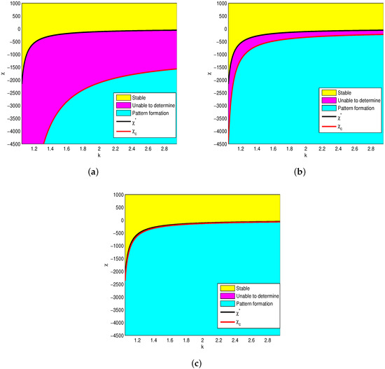
Figure 1. The effects of k on pattern formation for a different $l=1,3,10$. Critical prey-taxis coefficients ${\chi }^{*}$ and ${\chi }_c$ are given by Theorems 2 and 3: (a) $l=1$; (b) $l=3$; (c) $l=10$.

Firstly, because the expression of $Re\left(\lambda \right)$ is complex and it is difficult to judge intuitively its sign that determines the stability of positive constant steady state $(u_1,v_1)$, the plots of $Re\left(\lambda \right)$ with respect to n are presented in Figure 2, where $Re\left(\lambda \right)$ represents the real part of the eigenvalue given in (12). It follows from the theoretical analysis in Theorems 1 and 2 that positive constant steady state $(u_1,v_1)$ for (1) is unstable if the real part of eigenvalues $Re\left(\lambda \right)>0$, $(u_1,v_1)$ is stable if $Re\left(\lambda \right)<0$. Note that the sign of $Re\left(\lambda \right)$ mainly depends on the sign of $Q({\mu }_n,\chi )$, which also involves parameters $a,b,c,k,r,d_u,d_v,\chi ,l,n$. In order to illustrate how diffusion induces instability, we take the prey-taxis coefficient $\chi =0$ and $b=1.5$, $d_v=1$, $a=3$, $b=1$, $c=4$, $k=2$, $r=1$, $l=3$. If $d_u=0.1,0.001,0.0001,0.00001$ (see Figure 2a) and $d_u=1,10,100,1000,\text{10,000}$ (see Figure 2b), then $Re\left(\lambda \right)<0$ for all n. These results show that diffusion does not induce Turing instability. That is, when $\chi =0$, Model (1) will degenerate as a classical reaction–diffusion system without prey-taxis and its interior equilibrium $(u_1,v_1)$ possesses local stability (see Figure 3).

Figure 2. Plots of $Re\left(\lambda \right)$ with respect to n and fixed parameter values $a=3,b=1,c=4,k=2,r=1,l=3$. (a) The change trend of the real part of the eigenvalue when $d_u$ increases. (b) The change trend of the real part of the eigenvalue when $d_u$ decreases.

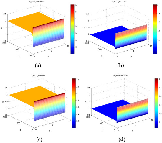
Figure 3. Numerical simulation of the solution $\left(u\right(x,t),v(x,t\left)\right)$ for Model (1) with $\chi =0$: (a,b) represent the population densities of predators; (c,d) represent the population densities of prey.

On the other hand, to illustrate how prey-taxis induces instability, we fix $d_u=1$, $d_v=10$. Hence, we have ${\chi }^{*}=-6.8246$ and ${\chi }_c=-9.0468$. By Theorem 3, there exists a bounded region $(-\infty ,-9.0468](\ni \chi )$ in which Turing instability occurs. According to Theorem 2, there also exists an unbounded region $(-6.8246,\infty )(\ni \chi )$ in which the stable equilibrium $(u_1,v_1)$ remains stable. Similarly, by varying the prey-taxis coefficient $\chi =0.001,10,\text{10,000}$ and $\chi =-6.8246,-7,-9.0468,-10$, we depict plots of $Re\left(\lambda \right)$ with respect to n in Figure 4, which indicates that if $\chi =0.001,10,\text{10,000}$ is positive, then $Re\left(\lambda \right)<0$ for all n (see Figure 4a); if $\chi =-7$ is greater than the critical prey-taxis coefficient ${\chi }_c$, then $Re\left(\lambda \right)<0$ for all n (see magenta curve in Figure 2b); if $\chi =-10$ is less than ${\chi }_c$, then $Re\left(\lambda \right)<0$ for some n (see red curve in Figure 2b). Figure 2b implies that $Re\left(\lambda \right)<0$ for all n (black line) when $\chi ={\chi }^{*}=-6.8246$ and $Re\left(\lambda \right)>0$ for $n=1$ (green curve in Figure 2b) when $\chi ={\chi }_c=-9.0468$. We take $\chi =-7$, which is larger than the critical prey-taxis coefficient ${\chi }_c$ and less than ${\chi }^{*}$. Then, $Re\left(\lambda \right)<0$ (magnetic line) for all n. Taking $\chi =-10$, we obtained simulation diagrams of the positive solutions $u(x,t)$ and $v(x,t)$ of Model (1) with Holling Type IV functional response (see Figure 5a,b), which indicates that the interior equilibrium $(u_1,v_1)$ is locally asymptotically stable. As stated before, the stability of the equilibrium point $(u_1,v_1)$ cannot be judged in the theoretical analysis. Interestingly, the numerical simulation shows that the equilibrium point $(u_1,v_1)$ is stable when $\chi =-7$ (see Figure 5c,d).

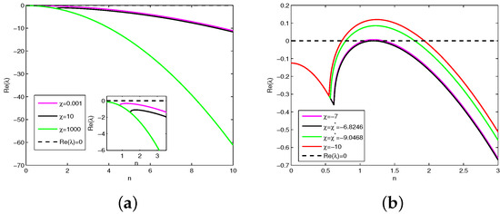
Figure 4. Plots of $Re\left(\lambda \right)$ with fixed parameter values $a=3,b=1,c=4,k=2,r=1,l=3$. (a) The change trend of the real part of the eigenvalue when $\chi$ increases. (b) The change trend of the real part of the eigenvalue when $\chi$ decreases.

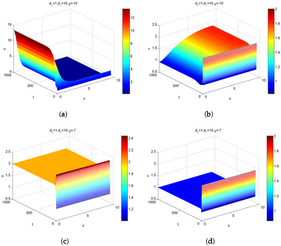
Figure 5. Numerical simulation of the solution $\left(u\right(x,t),v(x,t\left)\right)$ for Model (1) with the prey-taxis: (a,b) represent the population densities of predators; (c,d) represent the population densities of prey.

5. Conclusions

In this paper, we studied the asymptotic stability of the positive steady state of System (1) in a general framework. The stability of the predator–prey model is determined by the equilibrium points of the system. These equilibrium points can be stable or unstable, depending on the values of the model parameters. Stable equilibrium points represent a balanced coexistence between predators and prey, while unstable equilibrium points can lead to oscillatory behavior or population cycles. In addition to temporal patterns, the predator–prey model can also exhibit spatial patterns. These patterns arise due to spatial heterogeneity in the environment or movement behaviors of predators and prey. For example, if predators tend to aggregate in certain areas, it can lead to the formation of spatially localized prey populations. Spatial patterns can have important implications for the distribution and abundance of species in an ecosystem. The functional response $\mathcal{ϝ}\left(v\right)$ belongs to a large class of functions and it can take a complicated nonlinear form. Theoretically, based on the idea of Turing pattern, we have obtained necessary and sufficient conditions of prey-taxis-induced instability (Theorems 2 and 3 and Corollary 1), and we can see nonlocal terms promote linear stability (Corollary 2). In addition, we use the global bifurcation theorem to investigate steady-state solutions.

Numerically, the spatial–temporal behavior of the interacting species have been shown in one dimension. Particularly, we studied the specific model with Holling Type IV functional response and draw the following conclusions:

(1)

By substituting the specific value proposed in numerical simulation, Figure 3 shows that $(u_1,v_1)$ is stable for the corresponding reaction–diffusion system without prey-taxis.

(2)

By simple calculation, we can discover that ${\chi }^{*}=-6.8246$ and ${\chi }_c=-9.0468$. This means that $(u_1,v_1)$ remains locally asymptotically stable when System (1) possesses attractive ($\chi \in (0,\infty )$) prey-taxis. $(u_1,v_1)$ can also be locally asymptotically stable when the system (1) possesses repulsive prey-taxis with $(-6.8246,0)(\ni \chi )$ (see Figure 5c,d). When $(-9.0468,\infty )(\ni \chi )$, $(u_1,v_1)$ is unstable (see Figure 5a,b).

(3)

The numerical observations in Figure 1 are consistent with our theoretical results that the critical value of the necessary and sufficient conditions are almost similar when the study area is large enough (see Remark 2).

References

- Ruan, S.G.; Xiao, D.M. Global analysis in a predator-prey system with nonmonotonic functional response. SIAM J. Appl. Math. 2001, 61, 1445–1472. [Google Scholar] [CrossRef]
- Pang, Y.H.P.; Wang, M.X. Non-constant positive steady states of a predator-prey system with non-monotonic functional response and diffusion. Lond. Math. Soc. 2004, 88, 135–157. [Google Scholar] [CrossRef]
- Luo, D.; Wang, Q.R. Global bifurcation and pattern formation for a reaction–diffusion predator–prey model with prey-taxis and double Beddington–DeAngelis functional responses. Nonlinear Anal. Real World Appl. 2022, 67, 103638. [Google Scholar] [CrossRef]
- Yang, F.; Song, Y.L. Stability and spatiotemporal dynamics of a diffusive predator–prey system with generalist predator and nonlocal intraspecific competition. Math. Comput. Simul. 2022, 194, 159–168. [Google Scholar] [CrossRef]
- Ainseba, B.E.; Bendahmane, M.; Noussair, A. A reaction–diffusion system modeling predator–prey with prey-taxis. Nonlinear Anal. Real World Appl. 2008, 9, 2086–2105. [Google Scholar] [CrossRef]
- Huang, J.C.; Xiao, D.M. Analyses of bifurcations and stability in a predator-prey system with Holling type-IV functional response. Acta Math. Appl. Sin. 2004, 20, 167–178. [Google Scholar] [CrossRef]
- Hutson, V.; Lou, Y.; Mischaikow, K. Spatial heterogeneity of resources versus Lotk-Volterra dynamics. J. Differ. Equ. 2002, 185, 97–136. [Google Scholar] [CrossRef]
- Luo, D. Global bifurcation for a reaction-diffusion predator-prey model with Holling-II functional response and prey-taxis. Chaos Solitons Fractals 2021, 147, 110975. [Google Scholar] [CrossRef]
- Yan, X.; Maimaiti, Y.; Yang, W.B. Stationary pattern and bifurcation of a Leslie-Gower predator-prey model with prey-taxis. Math. Comput. Simul. 2022, 201, 163–192. [Google Scholar] [CrossRef]
- Jia, Y.F.; Wu, J.H.; Nie, H. The coexistence states of a predator-prey model with nonmonotonic functional response and diffusion. Acta Appl. Math. 2009, 108, 413–428. [Google Scholar] [CrossRef]
- Agarwal, M.J.; Pathak, R. Harvesting and Hopf Bifurcation in a prey-predator model with Holling Type IV Functional Response. Int. J. Math. Soft Comput. 2012, 2, 83–92. [Google Scholar] [CrossRef][Green Version]
- Liu, X.X.; Huang, Q.D. The dynamics of a harvested predator-prey system with Holling type IV functional response. Biosystems 2018, 169, 26–39. [Google Scholar] [CrossRef] [PubMed]
- Khnke, M.C.; Siekmann, B.; Hiromi, S.; Horst, M.A. A type IV functional response with different shapes in a predator-prey model. J. Theoret. Biol. 2020, 505, 110419. [Google Scholar] [CrossRef] [PubMed]
- Liu, X.; Huang, Q. Analysis of optimal harvesting of a predator-prey model with Holling type IV functional response. Ecol. Complex. 2020, 42, 100816. [Google Scholar] [CrossRef]
- Yeh, T.S. Classification of Bifurcation diagrams for a multiparameter diffusive logistic problem with Holling type-IV functional response. J. Math. Anal. Appl. 2014, 418, 183–304. [Google Scholar] [CrossRef]
- Shi, J.P.; Wang, X.F. On global bifurcation for quasilinear elliptic systems on bounded domains. J. Differ. Equ. 2009, 246, 2788–2812. [Google Scholar] [CrossRef]
- Xiang, T. Global dynamics for a diffusive predator-prey model with prey-taxis and classical Lotka-Volterra kinetics. Nonlinear Anal. Real World Appl. 2018, 39, 278–299. [Google Scholar] [CrossRef]
- Yousefnezhao, M.; Mohammai, S.A. Stability of a predator-prey system with prey taxis in a general class of functional responses. Acta Math. Sci. 2016, 36, 62–72. [Google Scholar] [CrossRef]
- Jin, H.Y.; Wang, Z.A. Global stability of prey-taxis systems. J. Differ. Equ. 2017, 262, 1257–1290. [Google Scholar] [CrossRef]
- Wang, X.L.; Wang, W.D.; Zhang, G.H. Global bifurcation of solutions for a predator-prey model with prey-taxis. Math. Methods Appl. 2015, 38, 431–443. [Google Scholar] [CrossRef]
- Chen, X.F.; Qi, Y.W.; Wang, M.X. A strongly coupled predator-prey system with non-monotonic functional response. Nonlinear Anal. 2007, 67, 1966–1979. [Google Scholar] [CrossRef]
- Du, Y.H.; Shi, J.P. A diffusive predator-prey model with a protection zone. J. Differ. Equ. 2006, 229, 63–91. [Google Scholar] [CrossRef]
- Dung, L.; Smith, H.L. Steady states of models of microbial growth and competition with chemotaxis. J. Math. Anal. Appl. 1999, 229, 295–318. [Google Scholar] [CrossRef][Green Version]
- Crandall, M.G.; Rabinowitz, P.H. Bifurcation from simple eigenvalues. J. Funct. Anal. 1971, 8, 321–340. [Google Scholar] [CrossRef]
- Wang, J.F.; Wu, S.N.; Shi, J.P. Pattern formation in diffusive predator-prey systems with predator-taxis and prey-taxis. Discret. Contin. Dyn. Syst. Ser.-B 2021, 26, 1273–1289. [Google Scholar] [CrossRef]
- Furter, J. Grinfeld, M. Local vs. non-local interactions in population dynamics. J. Math. Biol. 1989, 27, 65–80. [Google Scholar] [CrossRef]
- N, W.; Shi, J.; Wang, M. Global stability and pattern formation in a nonlocal diffusive Lotka–Volterra competition model. J. Differ. Equ. 2018, 264, 6891–6932. [Google Scholar]
- Wu, S.H.; Song, Y.L. Stability and spatiotemporal dynamics in a diffusive predator–prey model with nonlocal prey competition. Nonlinear Anal. Real World Appl. 2019, 48, 12–39. [Google Scholar] [CrossRef]
Disclaimer/Publisher’s Note: The statements, opinions and data contained in all publications are solely those of the individual author(s) and contributor(s) and not of MDPI and/or the editor(s). MDPI and/or the editor(s) disclaim responsibility for any injury to people or property resulting from any ideas, methods, instructions or products referred to in the content. |
© 2023 by the authors. Licensee MDPI, Basel, Switzerland. This article is an open access article distributed under the terms and conditions of the Creative Commons Attribution (CC BY) license (https://creativecommons.org/licenses/by/4.0/).