Abstract
The fifth-order WENO-Z scheme proposed by Borges et al., using a linear combination of low-order smoothness indicators, is designed to provide a low numerical dissipation to solve hyperbolic conservation laws, while the power q in the framework of WENO-Z plays a key role in its performance. In this paper, a novel global smoothness indicator with fifth-order accuracy, which is based on several lower-order smoothness indicators on two-point sub-stencils, is presented, and a new lower-dissipation WENO-Z scheme (WENO-NZ) is developed. The spectral properties of the WENO-NZ scheme are studied through the ADR method and show that this new scheme can exhibit better spectral results than WENO-Z no matter what the power value is. Accuracy tests confirm that the accuracy of WENO-Z with q = 1 would degrade to the fourth order at first-order critical points, while WENO-NZ can recover the optimal fifth-order convergence. Furthermore, numerical experiments with one- and two-dimensional benchmark problems demonstrate that the proposed WENO-NZ scheme can efficiently decrease the numerical dissipation and has a higher resolution compared to the WENO-Z scheme.
Keywords:
WENO-Z scheme; smoothness indicator; power parameter; fifth-order convergence; low dissipation; high resolution MSC:
65M06; 35L65
1. Introduction
As an important class of differential equation, the hyperbolic conservation equation has a wide application in scientific and engineering fields. One of the characteristics of this equation is that the solution may generate discontinuities even if its initial condition is smooth. For capturing the discontinuities, many numerical schemes, such as total variation diminishing schemes (TVD) [1,2,3], essentially non-oscillatory schemes (ENO) [4,5,6], weighted essentially non-oscillatory schemes (WENO) [7,8,9,10], etc., have been developed in recent decades. Among them, the WENO schemes have attracted great attention because they can not only obtain high-order solutions in smooth regions but also efficiently avoid spurious oscillatory near discontinuities.
The WENO scheme, first proposed by Liu et al. [7], provided one-order higher solutions than the ones of the rth-order ENO scheme [4,5] by using a convex combination of r candidate sub-stencils. Subsequently, Jiang and Shu [8] devised a new smoothness indicator for the WENO scheme by utilizing the Lagrange form of interpolation polynomials and proposed an efficient WENO-JS scheme. For the case r = 3, the resulting WENO-JS scheme is about twice as fast as the fourth-order ENO scheme on computational efficiency. Most importantly, this scheme can achieve optimal fifth-order accuracy. Henrick et al. [11] derived a sufficient condition for the fifth-order convergence and conducted a further analysis of the accuracy of WENO-JS. They found that the fifth-order WENO-JS scheme was only third-order accurate at first-order critical points. To increase the accuracy of the WENO scheme, different types of finite difference WENO schemes by reconstructing flux functions have been proposed [12,13,14,15,16], such as the RBF-WENO scheme, which was based on radial basis functions (RBFs) and the nonlinear weights of WENO-JS, which was first proposed by Guo and Jung in [12] and further developed by Abedian et al. [14,15]. On the other hand, some scholars developed various techniques to calculate the weights to improve the accuracy. For example, Henrick et al. [11] introduced a corrected mapping function to the nonlinear weights of WENO-JS and presented a WENO-M scheme which could restore the optimal convergence order even at critical points but was computationally expensive. Unlike the idea of WENO-M, Borges et al. [9] designed a fifth-order global smoothness indicator using the linear combination of low-order smoothness indicators and proposed an innovative WENO-Z scheme with lower numerical dissipation. Meanwhile, this scheme was able to obtain almost the same accurate numerical solution as WENO-M and reduced computation by 25%.
Castro et al. [17] extended the WENO-Z scheme to arbitrary (2r − 1) th odd-order accuracy by designing a general formula for the global smoothness indicator. However, it should be noted that the numerical dissipation of WENO-Z is dependent upon the power parameter q. For example, the scheme is less dissipative with q = 1 but will lose accuracy at critical points, such as the fifth-order WENO-Z is only fourth-order accurate at first-order critical points. In contrast, the scheme will decrease the correction of nonlinear weights and is more dissipative with q = 2. Hence, Borges et al. [9] suggested the power q taken to be 1 to maintain the low dissipation property. Recently, some studies [18,19,20,21,22,23] reconstructed a series of higher-order (even up to eighth-order) reference smoothness indicators to recover the optimal convergence for the low-dissipation WENO-Z scheme (means q = 1). Although numerical results confirmed that these modified schemes with higher-order smoothness indicators can achieve the desired accuracy in smooth regions including critical points, most of these works either used larger stencils or introduced user-tunable parameters, which led to the increased computation time or limited the application.
On the other hand, Acker et al. [24] concluded the important role of increasing the contribution of less-smooth candidate sub-stencils for increasing the resolution. They added an extra term to WENO-Z weights to increase the relevance of less-smooth sub-stencils and proposed a fifth-order WENO-Z+ scheme. In terms of the lrest progress, a new fifth-order WENO-Z scheme was developed by Tang et al. [25] to perform lower dissipation at discontinuities by constructing a selector that can identify the less-smooth sub-stencils. Unfortunately, the presented WENO schemes in [24,25] were still fourth-order accurate at critical points. Therefore, how to construct a low-dissipation WENO-Z scheme with better performances, which has overall fifth-order accuracy including critical points and a higher resolution near discontinuities, should be investigated thanks to its significant computational benefit.
In this study, we divide the five-point global stencil of the WENO scheme into four smaller two-point sub-stencils. By utilizing the local smoothness indicators of these sub-stencils, we devise a novel fifth-order global smoothness indicator and develop a WENO-NZ scheme. The numerical results demonstrate that the WENO-NZ scheme is less dissipative and can restore the optimal convergence order whatever the value of power q. Additionally, this scheme shows improved capability in capturing discontinuities and small scales and exhibits higher resolution compared to the WENO-Z scheme.
The rest of the paper is structured as follows: In Section 2, a brief overview of the fifth-order WENO-JS and WENO-Z schemes is discussed. In Section 3, an improved WENO-Z scheme is developed by using a new fifth-order global smoothness indicator. The performance comparison between WENO-Z and the proposed scheme for the one- and two-dimensional Euler equations is given in Section 4. Finally, the conclusions are presented in Section 5.
2. Numerical Method
The one-dimensional scalar hyperbolic conservation laws can be written as
here, is conservative variable, is flux. Consider the uniform grids () and define the cell interfaces as , is the uniform grid spacing, the semi-discretization of Equation (1) can be given as
here, is a numerical approximation to . The conservation property of Equation (2) is obtained by implicitly defining , and have
here, . Then, Equation (3) can be further approximated as
here, the numerical fluxes are higher order polynomial interpolations to and can be obtained by the WENO reconstruction.
In general, the flux is always split into two parts, and , to ensure numerical stability, such as
where and . In this paper, the global Lax–Friedrichs splitting is used, there are
where . Hence, can be computed as the positive and negative parts of , respectively, and have
In fact, and are symmetric with respect to for the WENO scheme, so we only describe how is approximated and the “+” will be dropped in the following content for convenience.
According to the construction of the fifth-order WENO scheme, the numerical flux can be given as
where the numerical fluxes are given by
Now, there are many different WENO construction techniques to compute the nonlinear weights , while the WENO-JS and WENO-Z are the most popular schemes.
2.1. WENO-JS Scheme
The well-known fifth-order WENO-JS scheme was proposed by Jiang and Shu [8], whose nonlinear weights were defined as
where are ideal weights that resulted in the fifth-order central upwind scheme, there are , , and respectively. The power is used to control the weights of less-smooth sub-stencils. The larger the q is set, the smaller the weight is obtained, but the scheme is more dissipative. Hence q = 2 is used for the WENO-JS scheme. is a positive sensitivity parameter used to avoid division by 0 and is adopted in this study. The local smoothness indicator is defined by
For the fifth-order WENO scheme (r = 3), the can be further expressed as
The Taylor expansions of Equation (12) at can be given as
Substituting Equation (13) into Equation (10), there are
Henrick et al. [11] concluded a detailed analysis of the accuracy of the fifth-order WENO scheme and derived a sufficient condition for the fifth-order convergence as follows
Equation (15) is further weakened as by Don et al. in [26]. Although it is not a necessary condition, it can be used as a simple criterion for designing nonlinear weights. Obviously, the weights of WENO-JS cannot meet the sufficient condition of Equation (15), especially at first-order critical points. It was reported that the WENO-JS scheme was only third-order accurate at critical points [11].
2.2. WENO-Z Scheme
Borges et al. [9] developed another fifth-order WENO scheme, called WENO-Z. They defined the nonlinear weights as
Here, is a global smoothness indicator given as
which with the following Taylor expansion
Substituting Equations (13) and (18) into Equation (16), then have
It can be found that the weights of WENO-Z with q = 1 do not meet the sufficient condition (15) at first-order critical points. Furthermore, Borges et al., confirmed that the WENO-Z scheme with q = 2 achieved fifth-order accuracy even at critical points. However, an increase in q resulted in more numerical dissipation of WENO-Z. Therefore, the power parameter q = 1 is suggested by Borges et al. and used by other scholars [18,19,20,21,22,23,24,25].
3. The New WENO-Z Scheme
Some works [20,21,22,23] demonstrated that constructing more higher-order smoothness indicators was useful in recovering the desired order for the low-dissipation WENO-Z scheme (means q = 1). Unlike these studies, we reconstructed a novel fifth-order global smoothness indicator with lower dissipation for the WENO-Z scheme to overcome its inherent limitations, such as its failure to balance the low-dissipation property and fifth-order convergence.
3.1. Construction of Novel Global Smoothness Indicator
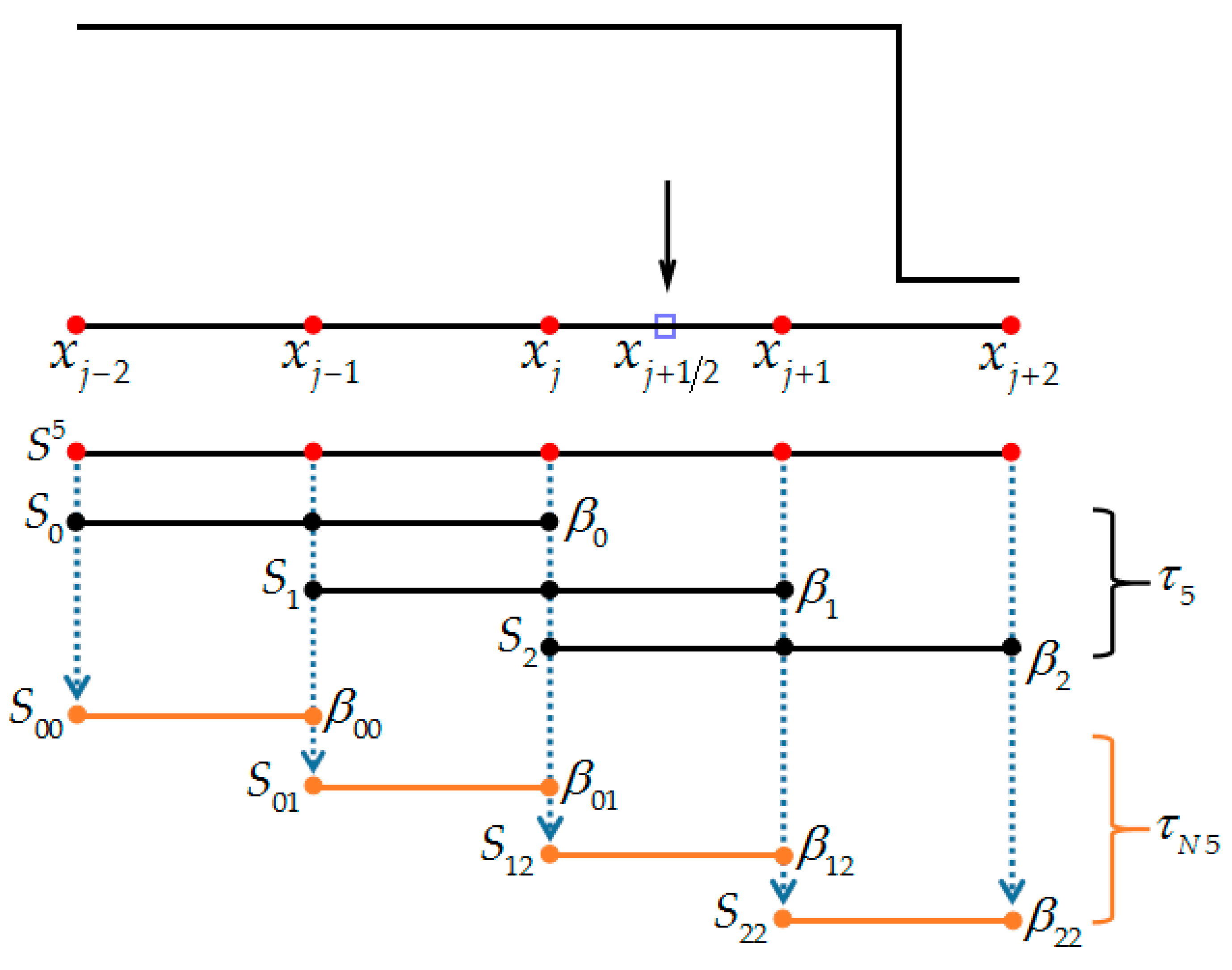
Within the framework for the original global smoothness indicator of WENO-Z, it is found that a discontinuity would affect the interpolation on the range of at least. Suppose a discontinuity is at any position to the left (or right) side of the center point , it would affect the interpolation on the three-point sub-stencil (or ). However, if a discontinuity is just right at , it would affect the interpolation of the entire five-point global stencil. To reduce the impact of the discontinuities on interpolation, we subdivided the global stencil into four smaller sub-stencils , each one only involving two points, as shown in Figure 1. In fact, these sub-stencils are generally used to construct the third-order WENO-Z scheme (r = 2).
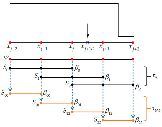
Figure 1.
The construction stencils of the new global smoothness indicator.
Based on these new smaller sub-stencils, a discontinuity will affect the nearby range at most, that is, two two-point sub-stencils. Furthermore, only a two-point sub-stencil where the discontinuity is located may be affected. From Equation (11), the smoothness indicators on sub-stencils can be computed as
with the following Taylor expansions
Consider the WENO scheme will lose accuracy at first-order critical points, in order to minimize the influence of the first-order derivative, meanwhile ensuring the global smoothness indicator has high-order accuracy, the form of a new fifth-order global smoothness indicator can be given as
the Taylor expansion of is as follows
3.1.1. Accuracy
Based on the nonlinear weights for the WENO-Z scheme, substituting instead of into Equation (16) can obtain a new weight, as follows
Substituting Equation (24) into Equation (8) results in a new WENO scheme, which is named WENO-NZ in this paper. Since has the same fifth-order accuracy as , similar to the accuracy analysis of WENO-Z, there are
which indicates that the WENO-NZ scheme has the same theoretical convergence accuracy as WENO-Z. A detailed analysis of the accuracy properties can be found in [9]. For simplicity, the WENO-Z and WENO-NZ schemes with different powers (q = 1 or 2) are, respectively, denoted as WENO-Z1, WENO-Z2, WENO-NZ1, and WENO-NZ2 in this paper.
3.1.2. Weights of Less-Smooth Sub-Stencils
In [9], numerical results made evident that the WENO-Z places higher weights on less-smooth sub-stencils than WENO-JS, this is the reason why WENO-Z achieves less dissipative results. The results in [24] also showed that it is important to increase the weights of less-smooth sub-stencils. Therefore, here is a numerical example to analyze the weights of less-smooth sub-stencils for the new WENO-NZ scheme.
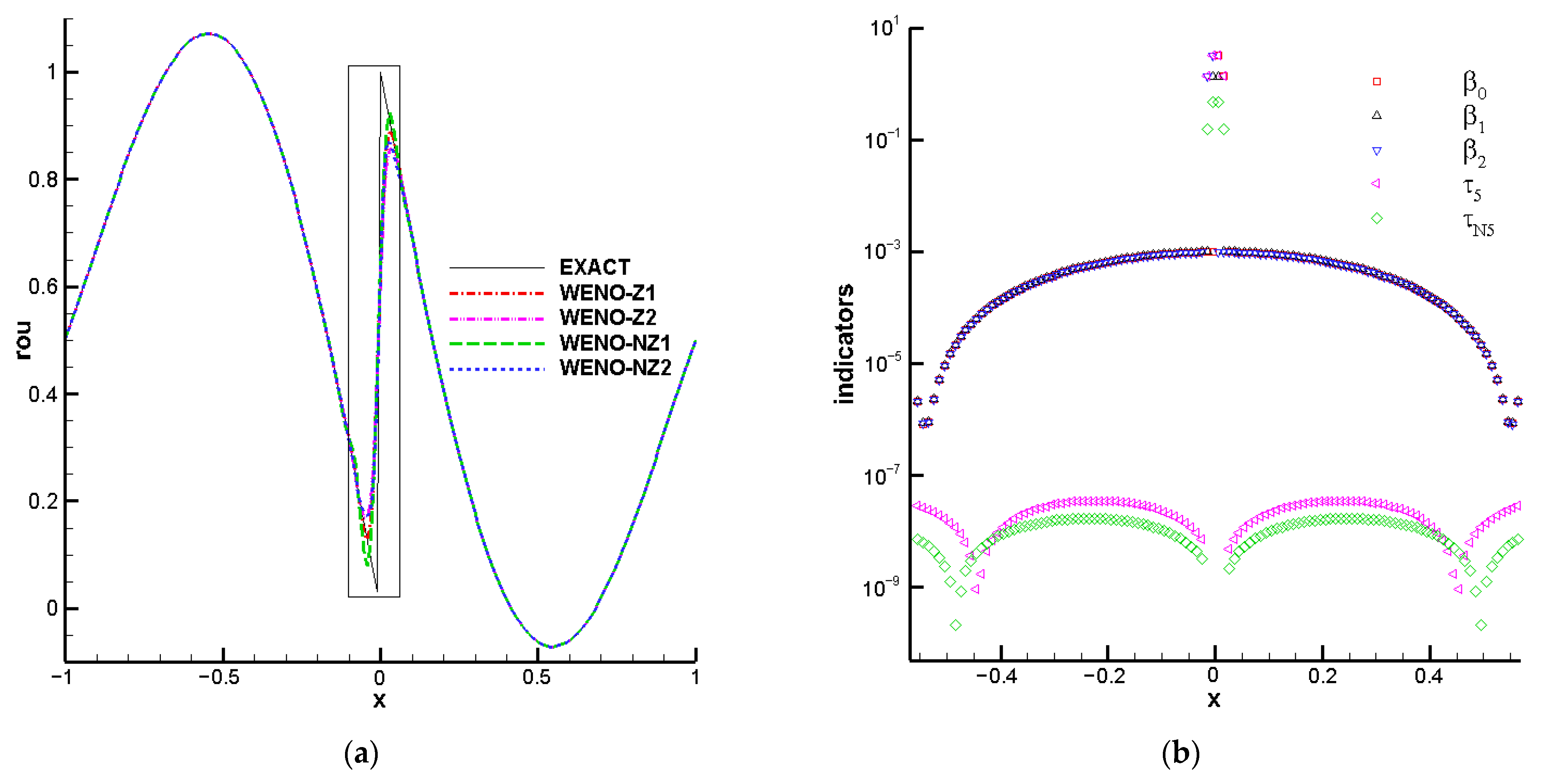
Consider the linear case of Equation (1) as follows
with the exact solution . This numerical example contains a jump discontinuity at x = 0, which is usually used to study the behavior of nonlinear weights in the smooth and discontinuous regions for the WENO scheme. We compute this numerical example to the final time t = 2.0 using N = 200 with periodic boundary, and the time step is set as . As shown in Figure 2a, the numerical results of WENO-NZ1 are the closest to that of the exact solution, and WENO-Z2 generates the most dissipation near discontinuities compared to others. Figure 2b gives the values of smoothness indicators at the initial step t = 0, i.e., , , and . We can see that is smaller than whether in smooth or discontinuous regions, hence, the WENO-NZ scheme is more accurate compared to WENO-Z.
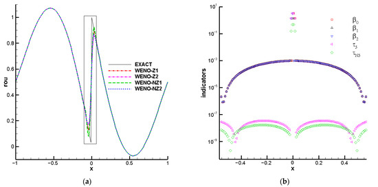
Figure 2.
Numerical solutions of the linear equation with discontinuity computed by different WENO schemes; (a) density distribution; (b) the values of smoothness indicators at t = 0.
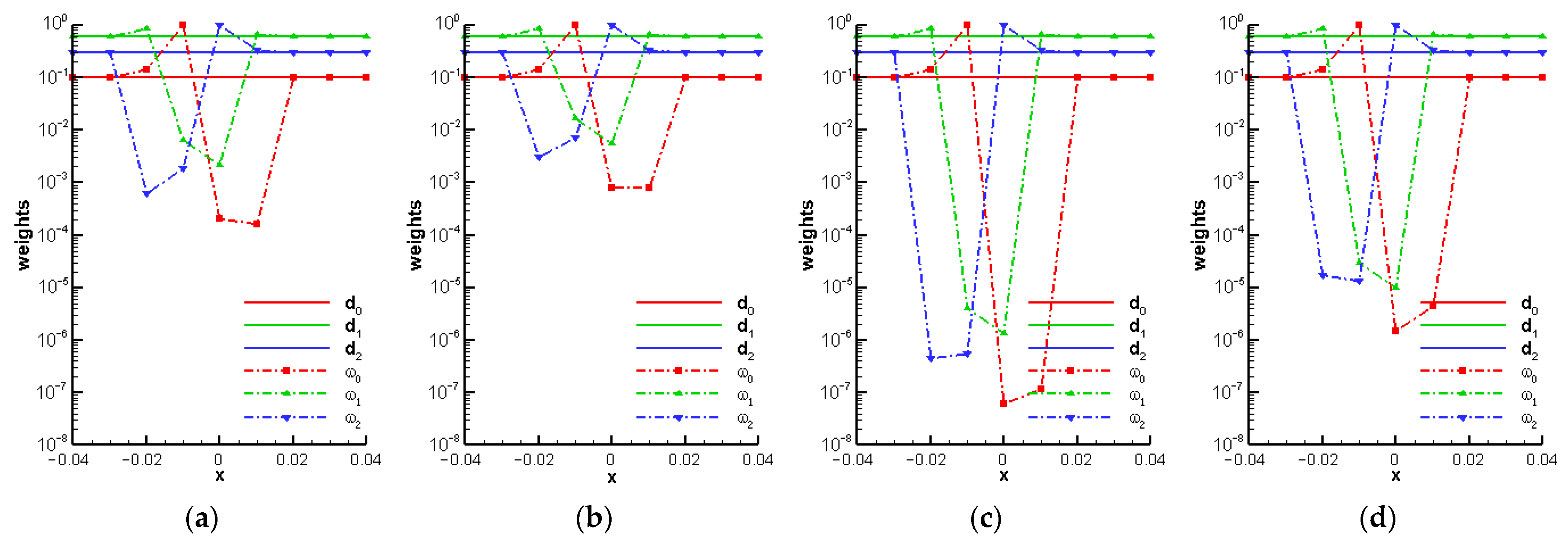
Figure 3 further provides the distributions of nonlinear weights for WENO-Z1, WENO-Z2, WENO-NZ1, and WENO-NZ2. As Figure 3 shows, at the point , where the discontinuity occurs for the first time, the is smaller than and , that is, the nonlinear weight of the less-smooth sub-stencil is smaller than that of smooth ones. It can be seen that the WENO-NZ assigns relatively larger weights to the less-smooth sub-stencils compared to the corresponding WENO-Z scheme. It can also be seen that the nonlinear weights of the WENO-NZ scheme are nearer to the ideal ones, resulting in the WENO-NZ scheme being closer to the central upwind scheme. As a result, this new scheme is less dissipative than the WENO-Z scheme.
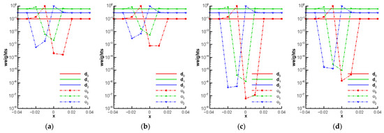
Figure 3.
The nonlinear weights of different schemes for the linear equation with discontinuity at t = 0; (a) WENO-Z1; (b) WENO-NZ1; (c) WENO-Z2; (d) WENO-NZ2.
3.2. The Spectral Properties of New Scheme
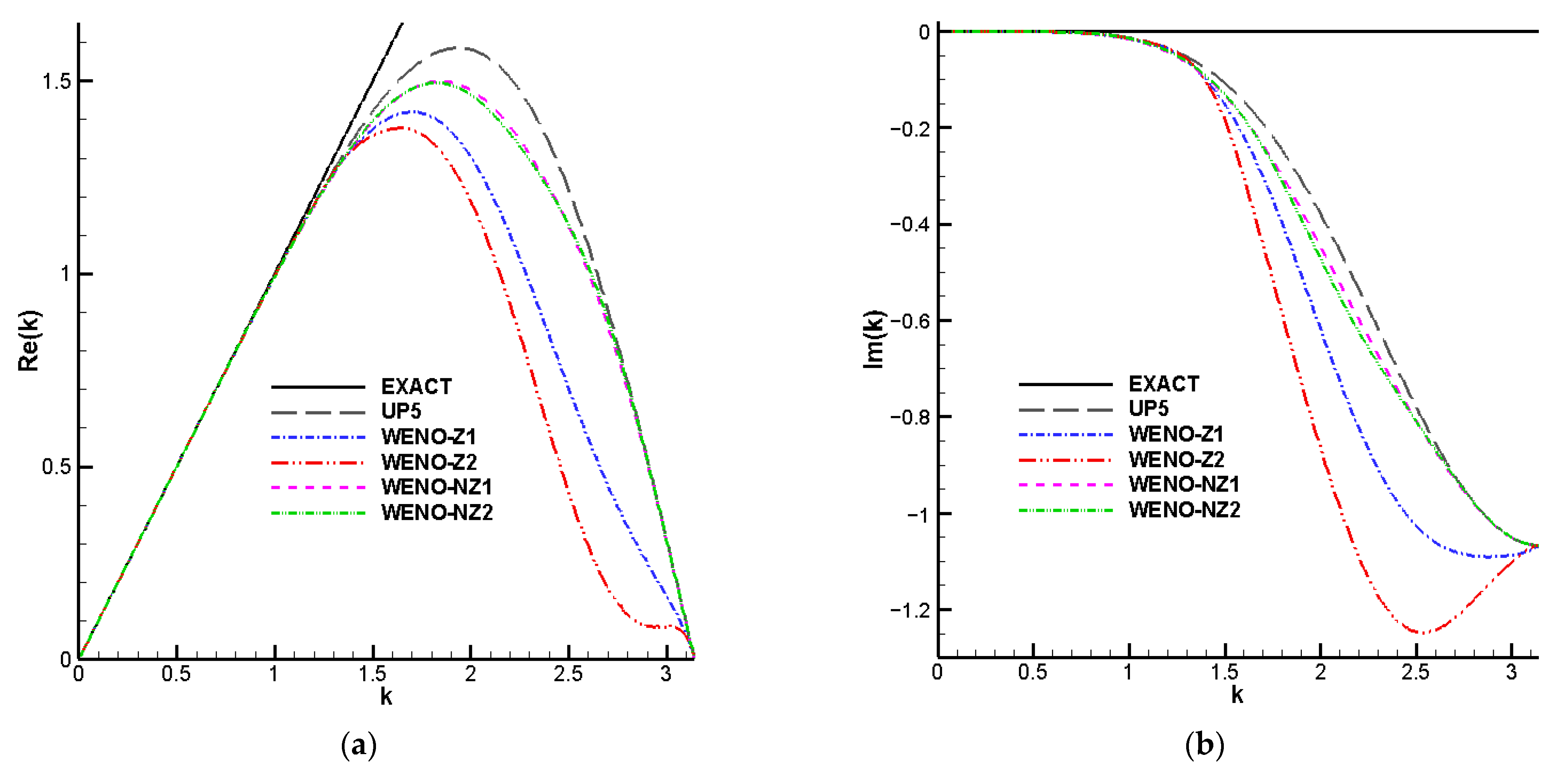
The spectral properties of the WENO-NZ scheme are studied using the ADR method proposed by Pirozzoli in [27]. As shown in Figure 4, it can be found that the dispersion and dissipation results of the WENO-NZ scheme are closer to the fifth-order upwind scheme (UP5) compared to WENO-Z, and the dispersion and dissipation curves of WENO-NZ are very similar to those of UP5. In addition, the spectral results of WENO-Z1 are better than those of WENO-Z2, but the results of WENO-NZ2 are nearly equivalent to that of WENO-NZ1, which implies that compared to WENO-Z, the WENO-NZ is a lower-dissipation scheme regardless of power q.
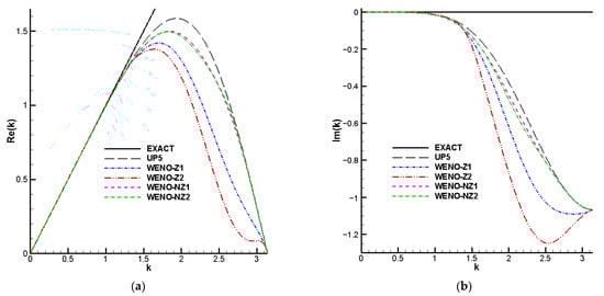
Figure 4.
The dispersion and dissipation properties of WENO-Z and WENO-NZ schemes; (a) dispersion; (b) dissipation.
4. Numerical Results
In this section, a series of typical numerical examples involving discontinuities and complex scale waves are computed to examine the accuracy, resolution, and low-dissipation properties of the proposed WENO-NZ scheme. The third-order Runge–Kutta method [1] is applied for time discretization with a CFL number of 0.5, as
where L is the spatial operator.
4.1. Linear Advection Problems
Consider the following linear advection problems
with the exact solution .
4.1.1. Accuracy Test
Case 1. The smooth initial condition is given as
This solution is computed up to t = 2.0 using the grids N = 40, 80, 160, 320, 640, and 1280. The time step is set as . In Table 1, the , , and errors, convergence orders, and CPU times are exhibited for the WENO-Z and WENO-NZ schemes with different powers, respectively. Here, the norm of errors is computed by

Table 1.
The errors, orders, and CPU times for linear advection problem with smooth initial condition computed by different WENO schemes.
It can be seen that all schemes can achieve fifth-order accuracy, but the CPU time of WENO-Z1 is the shortest compared to other schemes.
Case 2. The second initial condition for the accuracy test is given as
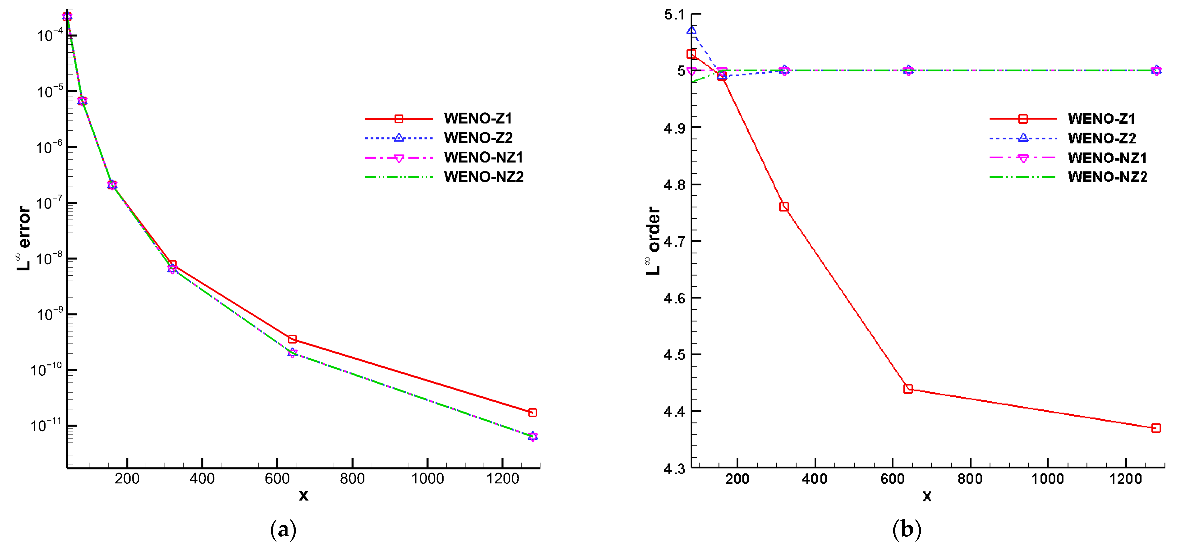
This solution has two critical points. We compute the solution up to t = 2.0 using the grids N = 40, 80, 160, 320, 640, and 1280 with . The , , and errors, convergence orders, and CPU times for different schemes are exhibited in Table 2. It can be found that the errors of WENO-Z2, WENO-NZ1, and WENO-NZ2 are one order of magnitude lower than WENO-Z1. For ease of observation, Figure 5 gives the line graphs of errors and orders. From Figure 5a, it can be seen that the errors of WENO-Z2, WENO-NZ1, and WENO-NZ2 are almost the same and are smaller than those of WENO-Z1. Moreover, it can also be seen from Figure 5b that the order of WENO-Z1 is only fourth-order accurate with the increase in grid numbers, while other schemes can achieve the desired fifth-order accuracy. Therefore, WENO-NZ proves to be a precise and effective scheme.
Table 2.
The errors, orders, and CPU times for the linear advection problem with two critical points were computed by different WENO schemes.
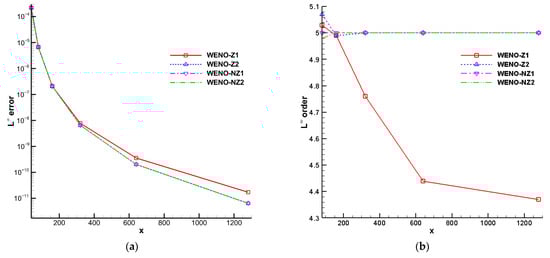
Figure 5.
The numerical results for the linear advection problem with two critical points computed by different WENO schemes; (a) errors; (b) orders.
4.1.2. Linear Problem with Several Critical Points
The initial condition is given as
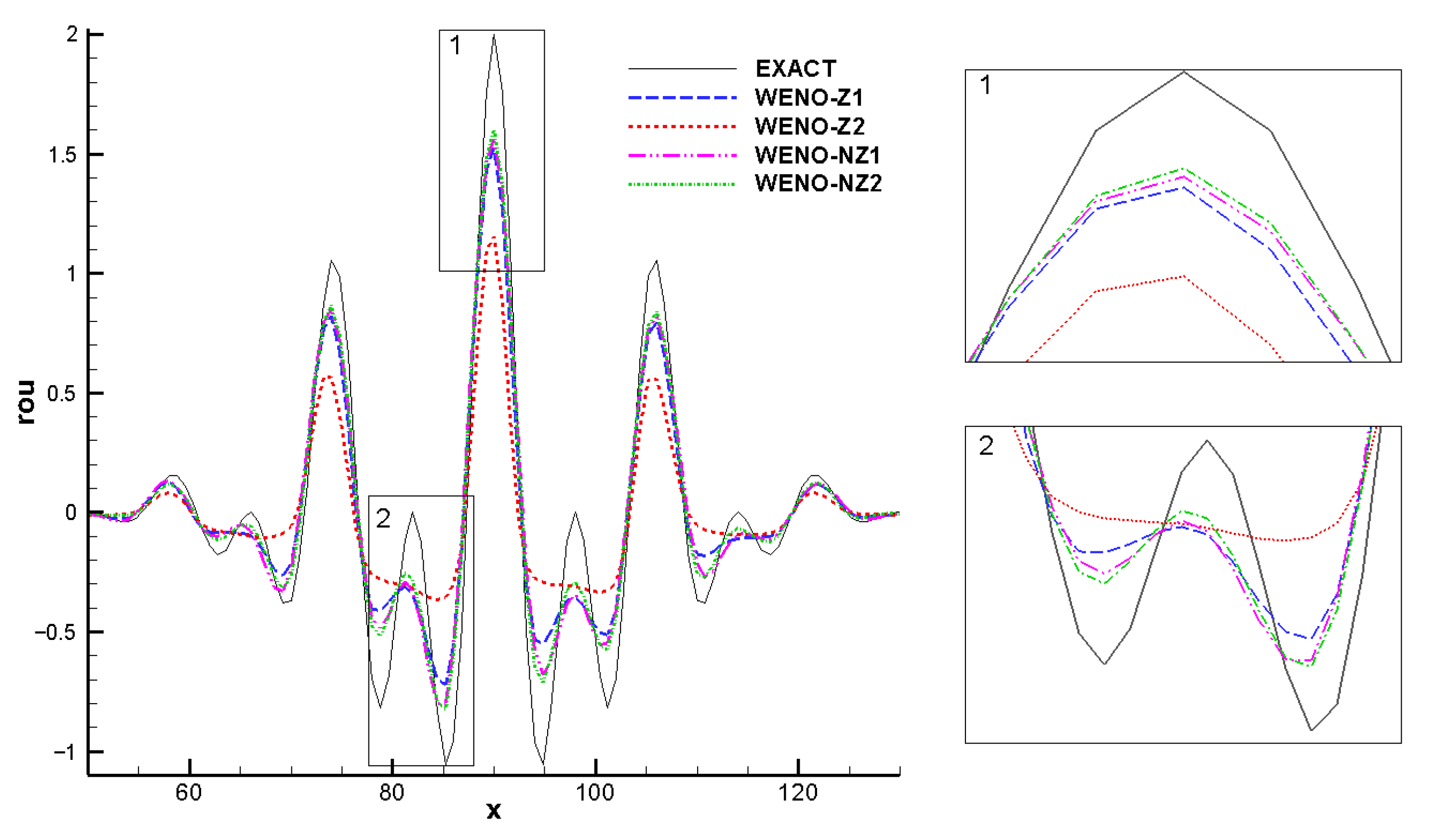
This solution involves several critical points and is often used to test the numerical dissipation of WENO schemes. The solution is calculated by using N = 100 until the final time t = 400 with . As Figure 6 shows, the numerical results of WENO-NZ are closer to the exact solution than WENO-Z, which again reveals that the WENO-NZ is a lower-dissipation scheme. In addition, the numerical results of WENO-NZ2 are almost comparable or even better than those of WENO-NZ1 at critical points, this is because the weights of WENO-NZ1 cannot satisfy the fifth-order convergence sufficient condition at critical points, but WENO-NZ2 can satisfy and also provide the lower dissipation.
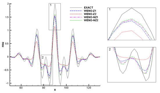
Figure 6.
Numerical solutions of linear advection problem with several critical points computed by different WENO schemes.
4.2. One-Dimensional Euler Problems
The one-dimensional Euler equation can be written as
with
Here,, p, , and E are the density, pressure, x-velocity, and total energy, respectively. The total energy is given as with the ratio of specific heat . In this subsection, the extrapolation boundary conditions are adopted and the “exact” solution is computed using the fifth-order WENO-JS scheme with N = 2000.
4.2.1. SOD Problem
The initial conditions of the sod problem are as follows
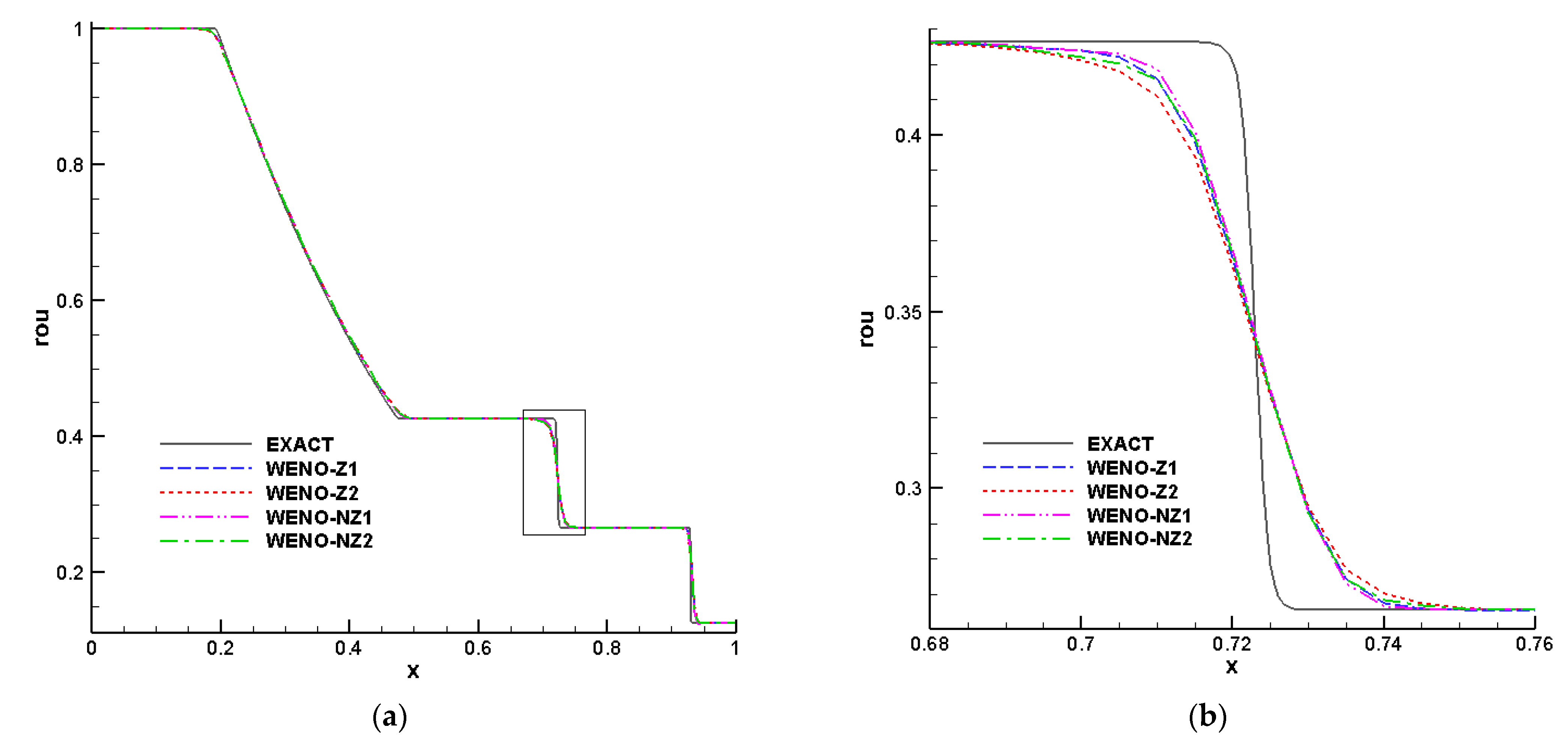
This problem is run up to the final time t = 0.25 with N = 200, resulting in a shock wave, a contact discontinuity, and an expansion wave. From Figure 7a, all the schemes can both simulate the sod problem without oscillatory. The zoom-in results of contact discontinuity for different schemes are displayed in Figure 7b. It can be found that the WENO-NZ1 scheme can capture the contact discontinuities well and is slightly closer to the “exact” solution than the others.
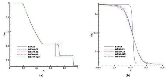
Figure 7.
Numerical solutions of sod problem computed by different schemes; (a) density distribution; (b) a zoom of contact discontinuity.
4.2.2. Lax Problem
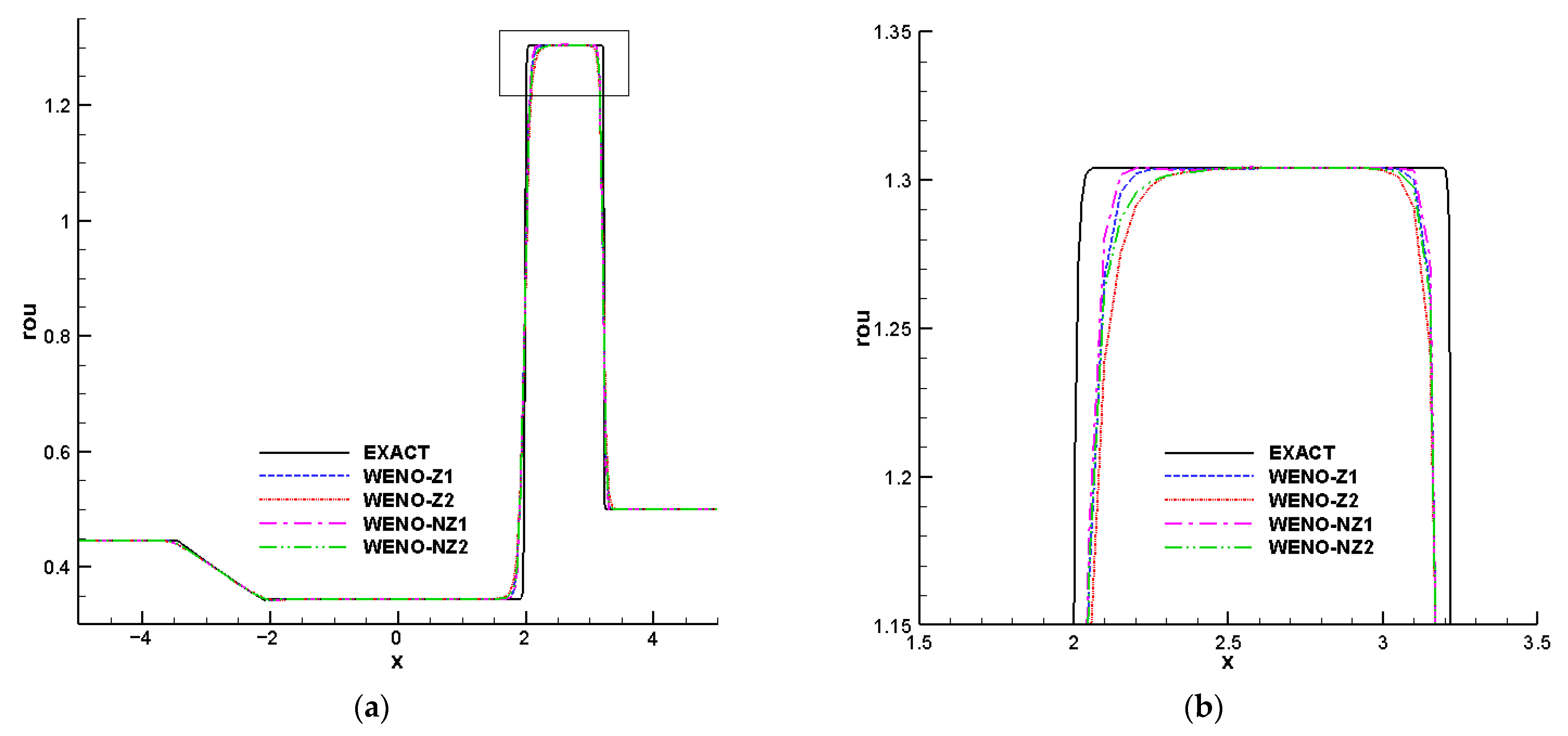
The initial conditions of the lax problem are as follows
Figure 8 shows a comparison of different schemes with N = 200 at t = 1.3. From Figure 8a, we can see that all schemes can pass through the sound velocity point smoothly. However, it can be seen from Figure 8b that, in comparison to WENO-Z, the corresponding WENO-NZ scheme provides lower numerical dissipation.
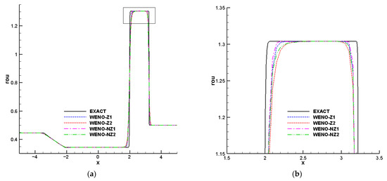
Figure 8.
Numerical solutions of lax problem computed by different schemes; (a) density distribution; (b) a zoom of discontinuity.
4.2.3. Shu–Osher Problem
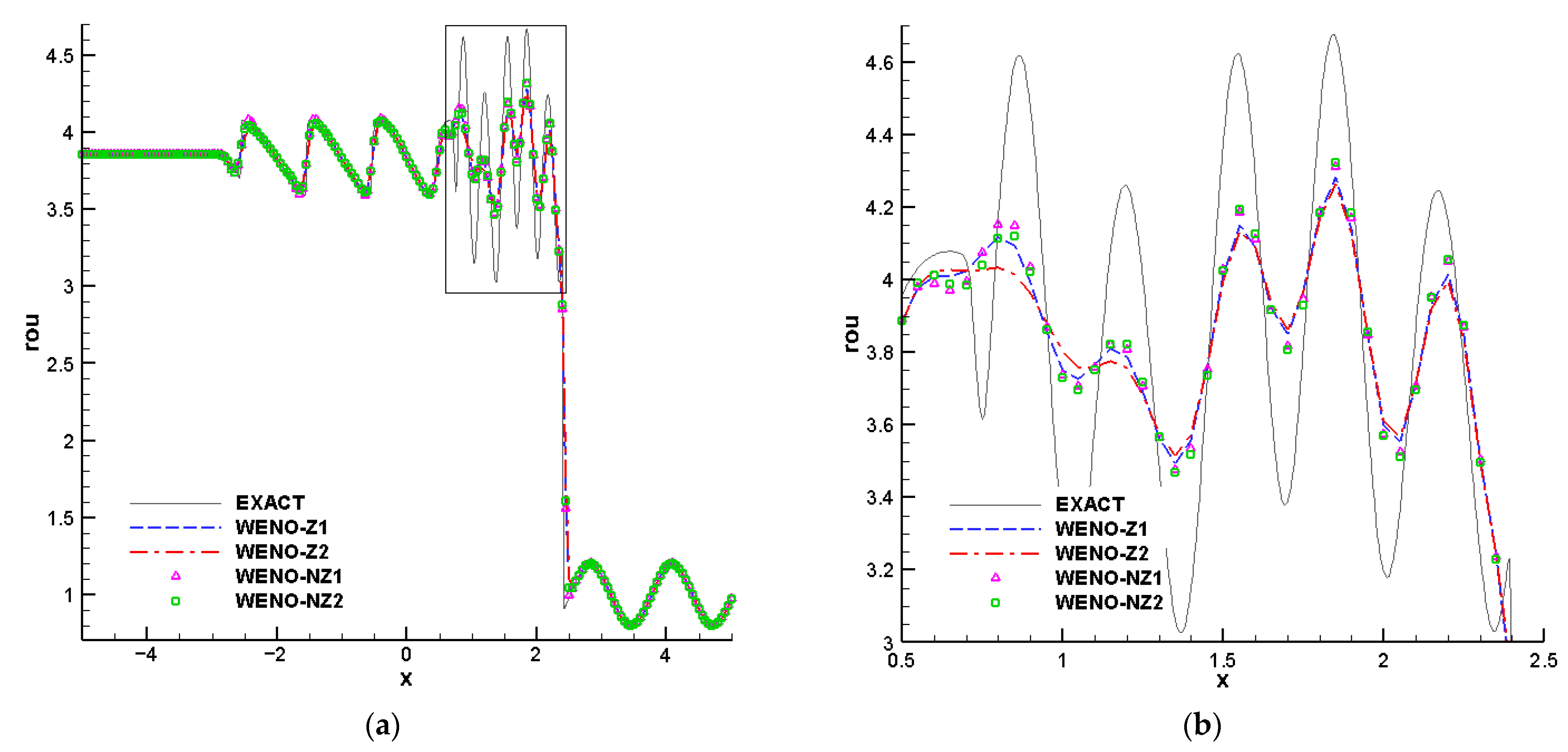
The initial conditions of Shu–Osher shock-entropy wave interaction are as follows
This problem involves the presence of shocklets and fine-scale structures, it is frequently utilized to study the stability of capturing shocks. We solve this problem until t = 1.8 using N = 200 and present the density results for different schemes in Figure 9. Examining the high-frequency wave region as depicted in Figure 9b, it can be seen that the WENO-NZ scheme performs a better job in approaching the “exact” solution compared to WENO-Z. Especially, in the area [1.3, 2.3], the numerical dissipation of WENO-NZ2 is even equivalent to WENO-NZ1. Based on the observations from Figure 7, Figure 8 and Figure 9, it can be concluded that the proposed WENO-NZ scheme effectively reduces numerical dissipation and is capable of stable shock capture.
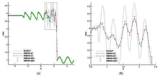
Figure 9.
Numerical solutions of the Shu-Osher problem computed by different schemes; (a) density distribution; (b) a zoom of the high-frequency wave.
4.3. Two-Dimensional Euler Problems
The two-dimensional Euler equation can be written as
with
Here, , p, , and v are the density, pressure, x- and y-velocity, respectively. The total energy E is given as with the ratio of specific heat , unless otherwise indicated.
4.3.1. Riemann Problem
The initial conditions of the two-dimensional Riemann problem are as follows
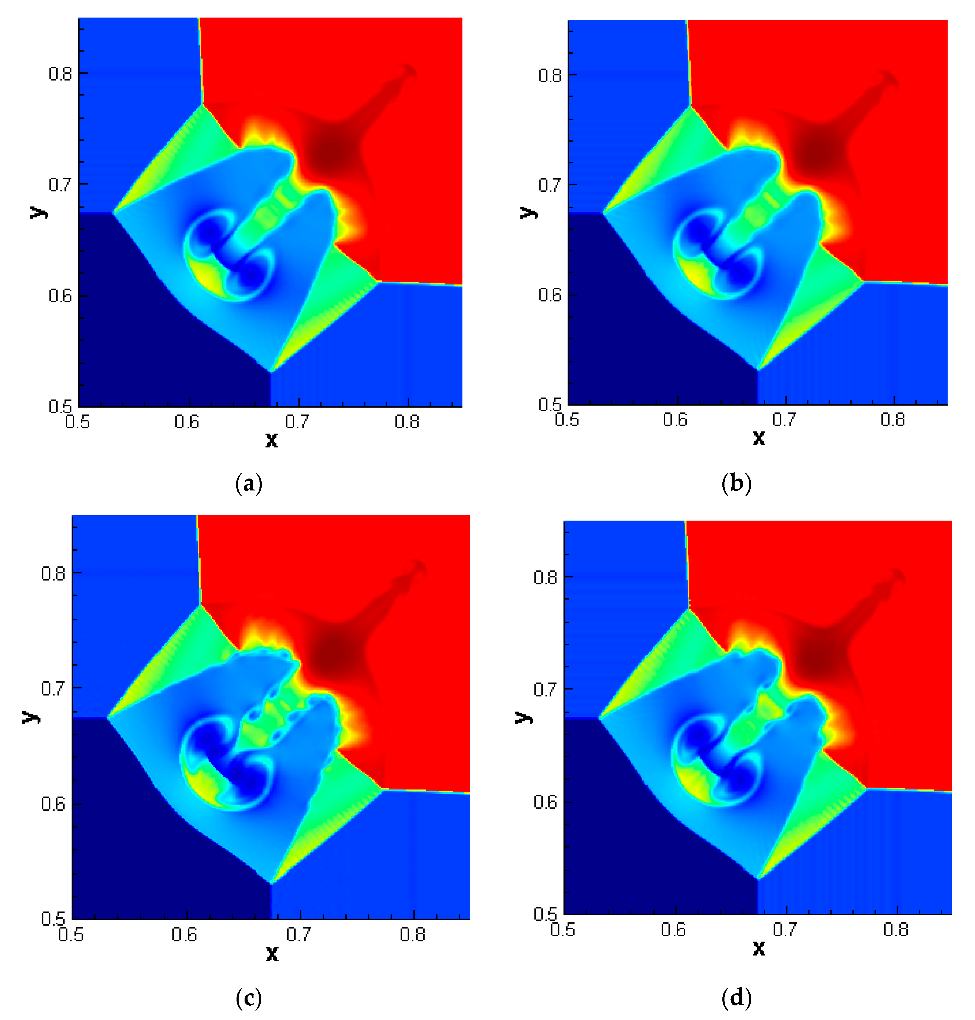
With the computational domain , this problem involves some vortex structures generated by Kelvin–Helmholtz instability and is often used to investigate numerical dissipation. Figure 10 gives the density profiles computed by different schemes at t = 0.3 with uniform meshes of 800 × 800 and zero-order extrapolation boundary conditions. As depicted in the results, the WENO-NZ scheme captures reflected shock waves more accurately and clearly than WENO-Z, which indicates that the numerical dissipation of WENO-NZ is smaller than that of WENO-Z. Among these schemes, WENO-NZ1 exhibits the richest vortex structures. However, it is important to note that when the time is pushed forward to longer, WENO-NZ1 will break the symmetrical roll-up of the Kelvin–Helmholtz instability because its numerical dissipation is too small. Fortunately, WENO-NZ2 not only performs well but also can maintain symmetry to solve this problem.
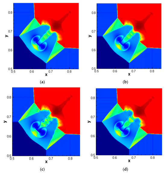
Figure 10.
Numerical solutions of 2D Riemann problem computed by different schemes; (a) WENO-Z1; (b) WENO-Z2; (c) WENO-NZ1; (d) WENO-NZ2.
4.3.2. Double Mach Reflection Problem
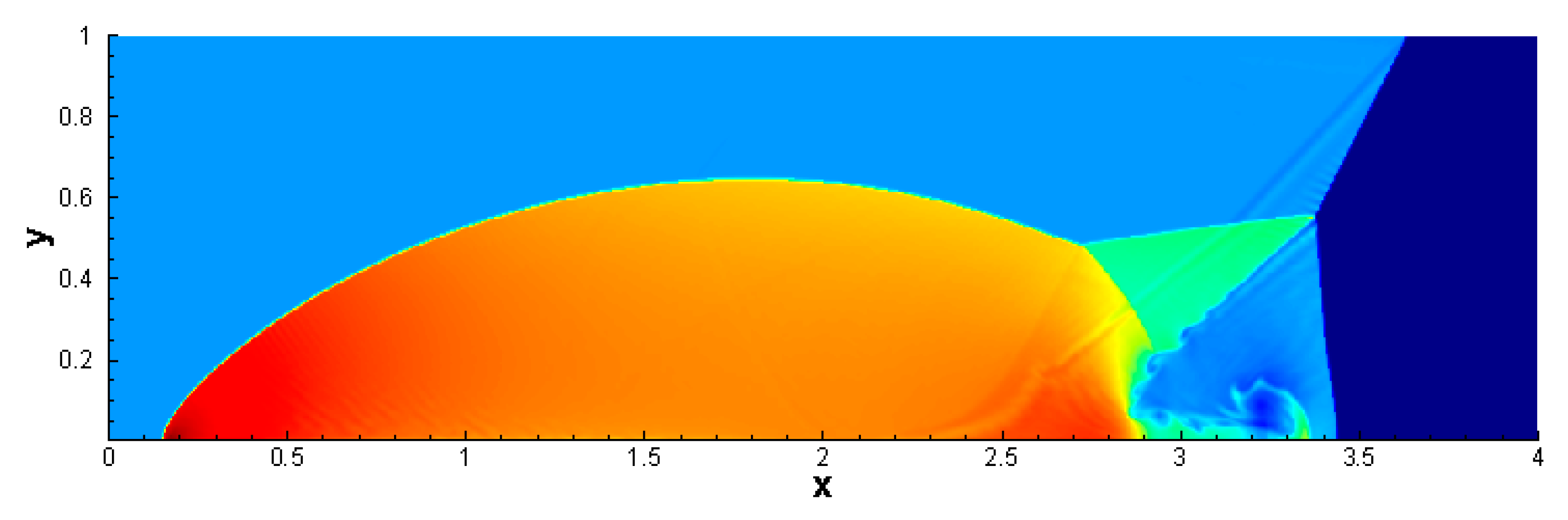
The double Mach reflection problem depicts a right-moving Mach 10 shock wave with an angle of 60° hitting a reflecting wall at x = 1/6, which lies at the bottom of the computational domain . This results in the formation of complex flow patterns, including shock wave reflections and vortex structures (see Figure 11, which is computed by the WENO-Z1 scheme using grids to t = 0.25). The initial conditions are as follows
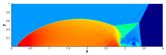
Figure 11.
Numerical solutions of double Mach reflection problem computed by the WENO-Z1 scheme with uniform meshes of .
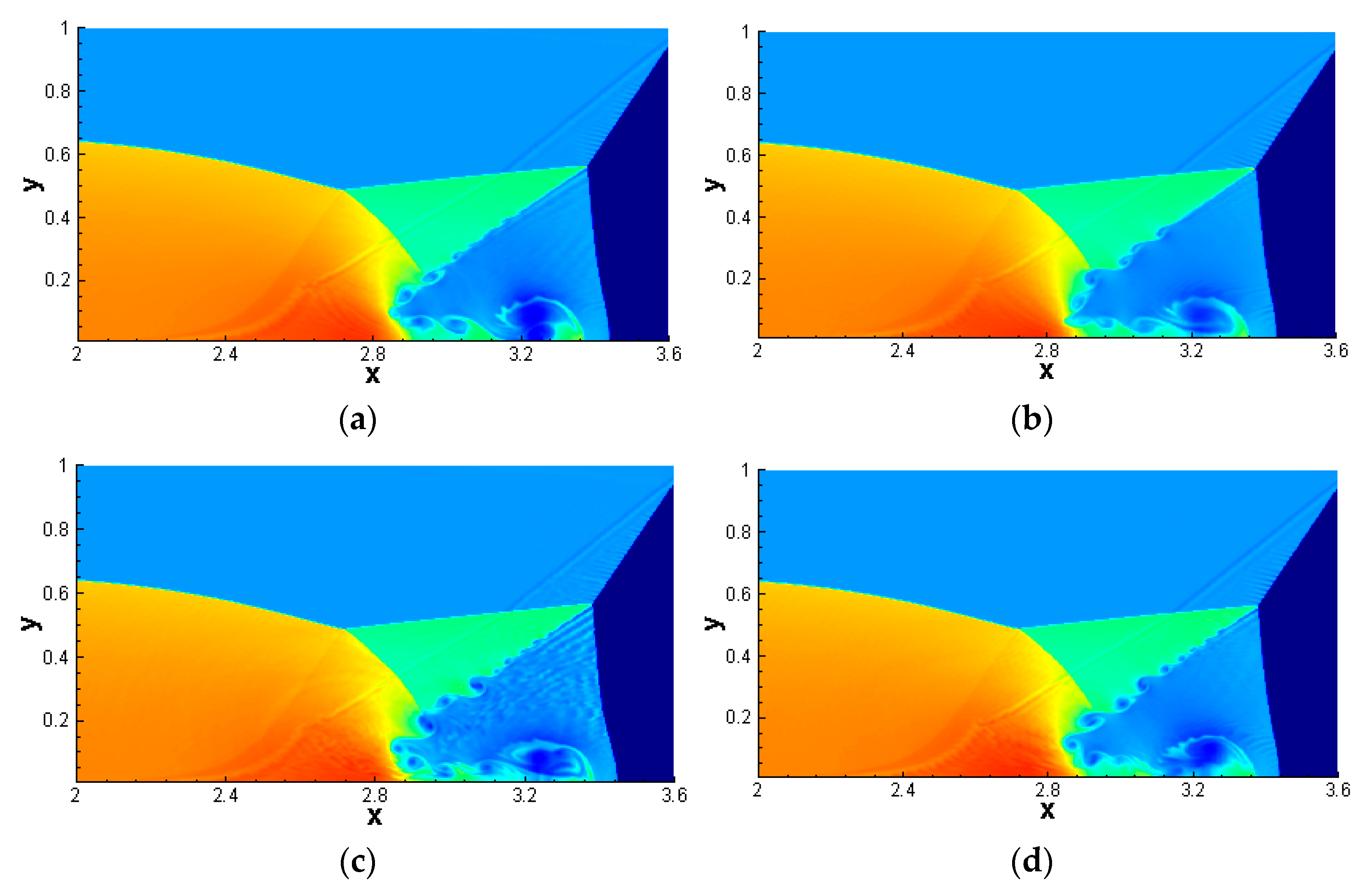
The exact post shock condition is imposed from x = 0 to x = 1/6 and the reflective boundary condition is used for the rest of the bottom. The boundary condition at the top corresponds to the exact motion of a Mach 10 shock, while the left and right boundaries are subject to inflow and outflow boundary conditions, respectively. Figure 12 shows the density results near the Mach stem computed by different schemes with uniform meshes of . It can be seen that the WENO-NZ scheme depicts richer vortex structures and has a higher resolution compared with the WENO-Z scheme. In addition, Figure 13 further shows the local density profiles computed by using denser meshes of , it can be also seen that the WENO-NZ scheme still performs better results than WENO-Z. However, Figure 12 and Figure 13 both show that WENO-NZ1 exhibits Gibbs oscillation due to its numerical dissipation being too small, while WENO-NZ2 does not. Based on the numerical results of the Riemann problem and double Mach reflection problem, it is not difficult to find that the numerical dissipation is too small and would not be a good choice for some two-dimensional problems involving small vortex structures, so we suggest taking the power to be q = 2 for WENO-NZ to calculate these problems.
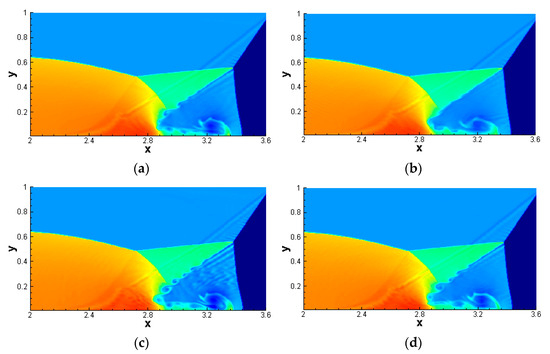
Figure 12.
A zoom of numerical solutions near the Mach stem for the double Mach reflection problem, which is computed by different schemes with uniform meshes of ; (a) WENO-Z1; (b) WENO-Z2; (c) WENO-NZ1; (d) WENO-NZ2.
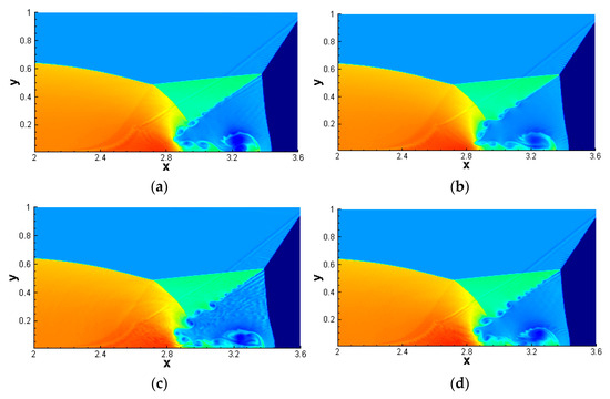
Figure 13.
A zoom of numerical solutions near the Mach stem for the double Mach reflection problem, which is computed by different schemes with uniform meshes of ; (a) WENO-Z1; (b) WENO-Z2; (c) WENO-NZ1; (d) WENO-NZ2.
4.3.3. Rayleigh–Taylor Instability Problem
The Rayleigh–Taylor instability problem describes the interface instability when a heavy fluid accelerates into a light one, whose initial conditions are given as
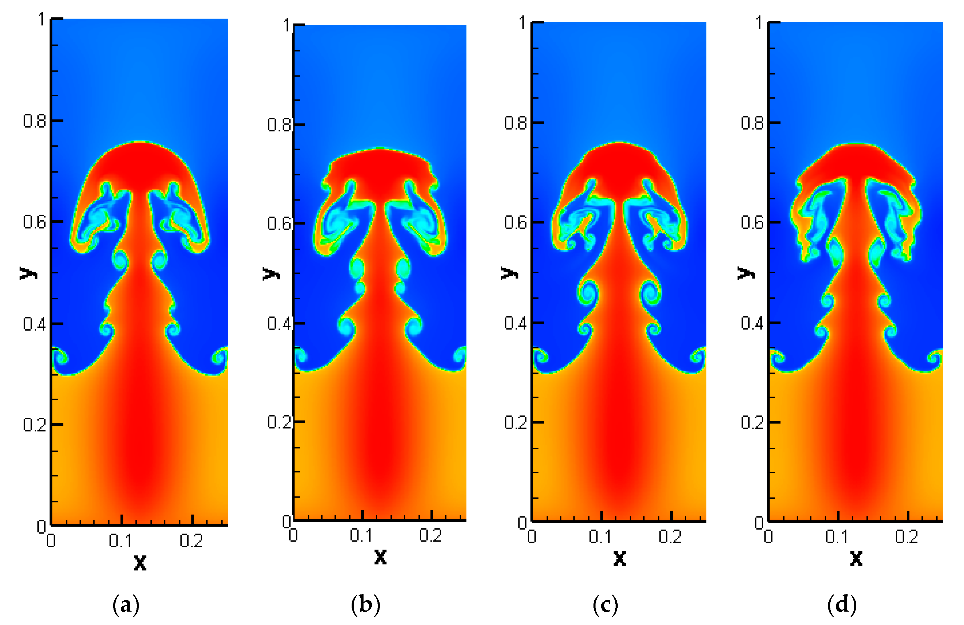
The computational domain is and the ratio of specific heat is . The reflective boundary conditions are employed for the left and right boundaries. The boundary conditions on the top and bottom boundaries are given as and , respectively. Figure 14 gives the density results computed by different schemes with meshes
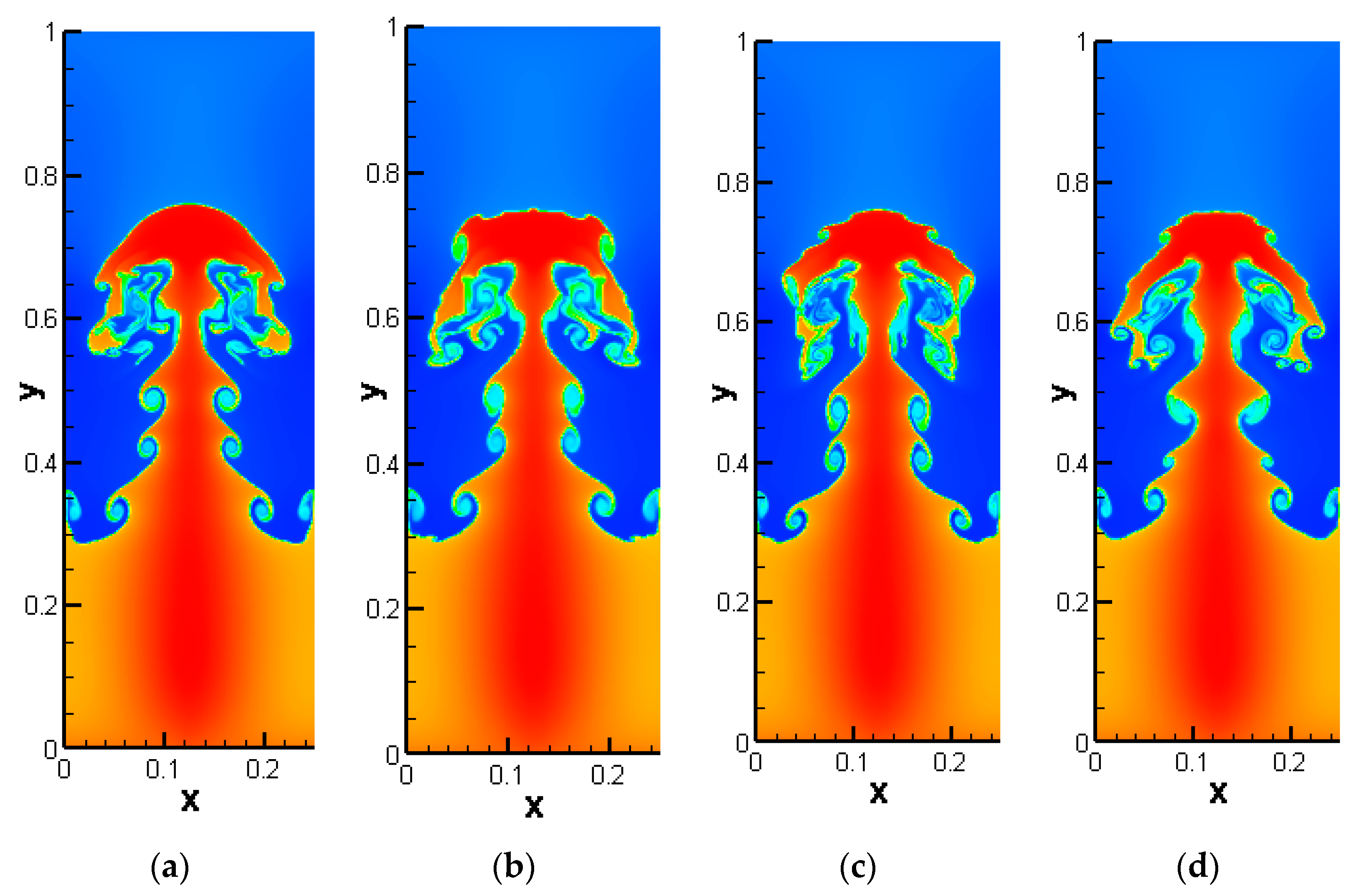
of until t = 1.95. It is apparent that all schemes are able to maintain the symmetry of the growth of instability. Compared to WENO-Z, the proposed WENO-NZ scheme displays more finer microstructures. Figure 15 further gives the density results computed to t = 1.95 by using denser meshes of . Obviously, the WENO-NZ scheme exhibits a greater richness of complex vortex structures and better resolution than the WENO-Z scheme.
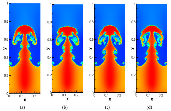
Figure 14.
Numerical solutions of Rayleigh–Taylor instability problem computed by different schemes with uniform meshes of ; (a) WENO-Z1; (b) WENO-Z2; (c) WENO-NZ1; (d) WENO-NZ2.

Figure 15.
Numerical solutions of Rayleigh–Taylor instability problem computed by different schemes with uniform meshes of ; (a) WENO-Z1; (b) WENO-Z2; (c) WENO-NZ1; (d) WENO-NZ2.
5. Conclusions
In this study, we modified the global smoothness indicator of the fifth-order WENO-Z scheme to improve its performance. First, the five-point global stencil was subdivided into four smaller sub-stencils that are usually used to construct the third-order WENO-Z scheme. Based on these lower-order smoothness indicators, a novel global smoothness indicator with fifth-order accuracy was reconstructed, which resulted in the new WENO-NZ scheme. The results from ADR analysis implied that the proposed scheme was a low-dissipation scheme, whatever the value of power q. Accuracy tests showed that the WENO-NZ scheme with either q = 1 or q = 2 could achieve fifth-order accuracy even at critical points. Compared with the WENO-Z scheme, although the WENO-NZ had the same theoretical convergence accuracy, the WENO-Z failed to balance the low-dissipation property and fifth-order convergence. Moreover, a series of one- and two-dimensional benchmark problems demonstrated the WENO-NZ scheme showed lower numerical dissipation and better resolution than WENO-Z. However, for some two-dimensional problems involving small vortex structures, the power q was best to be 2 for the WENO-NZ scheme since the numerical dissipation was too small to suppress oscillation when q = 1.
Author Contributions
Conceptualization, S.H. and M.L.; methodology, S.H. and M.L.; software, S.H.; validation, S.H.; formal analysis, S.H. and M.L.; investigation, S.H.; resources, S.H.; data curation, S.H.; writing—original draft preparation, S.H.; writing—review and editing, S.H. and M.L.; visualization, S.H.; supervision, M.L.; project administration, M.L.; funding acquisition, M.L. All authors have read and agreed to the published version of the manuscript.
Funding
This research was funded by National Natural Science Foundation of China under grant no. (11971411).
Data Availability Statement
Not applicable.
Conflicts of Interest
The authors declare no conflict of interest.
References
- Harten, A. High resolution schemes for hyperbolic conservation laws. J. Comput. Phys. 1983, 49, 357–393. [Google Scholar] [CrossRef]
- Toro, E.F.; Billett, S.J. Centred TVD schemes for hyperbolic conservation laws. IMA J. Numer. Anal. 2000, 20, 47–79. [Google Scholar] [CrossRef]
- Tang, S.J.; Li, M.J. Construction and application of several new symmetrical flux limiters for hyperbolic conservation law. Comput. Fluids 2020, 93, 104741. [Google Scholar] [CrossRef]
- Harten, A.; Osher, S.; Engquist, B.; Chakravarthy, S.R. Some results on uniformly high-order accurate essentially nonoscillatory schemes. Appl. Numer. Math. 1986, 2, 347–377. [Google Scholar] [CrossRef]
- Harten, A.; Engquist, B.; Osher, S.; Chakravarthy, S.R. Uniformly high order accurate essentially non-oscillatory schemes, III. J. Comput. Phys. 1987, 71, 231–303. [Google Scholar] [CrossRef]
- Shu, C.W.; Osher, S. Efficient implementation of essentially non-oscillatory shock-capturing schemes. J. Comput. Phys. 1988, 77, 439–471. [Google Scholar] [CrossRef]
- Liu, X.D.; Osher, S.; Chan, T. Weighted essentially non-oscillatory schemes. J. Comput. Phys. 1994, 115, 200–212. [Google Scholar] [CrossRef]
- Jiang, G.S.; Shu, C.W. Efficient implementation of weighted ENO schemes. J. Comput. Phys. 1996, 126, 202–228. [Google Scholar] [CrossRef]
- Borges, R.; Carmona, M.; Costa, B.; Don, W.S. An improved weighted essentially non-oscillatory scheme for hyperbolic conservation laws. J. Comput. Phys. 2008, 227, 3191–3211. [Google Scholar] [CrossRef]
- Tang, S.J.; Li, M.J. Novel functional weights for improving the third-order WENO schemes. Int. J. Numer. Meth. Fluids 2021, 93, 3131–3150. [Google Scholar] [CrossRef]
- Henrick, A.K.; Aslam, T.D.; Powers, J.M. Mapped weighted essentially non-oscillatory schemes: Achieving optimal order near critical points. J. Comput. Phys. 2005, 207, 542–567. [Google Scholar] [CrossRef]
- Guo, J.; Jung, J.H. Radial basis function ENO and WENO finite difference methods based on the optimization of shape parameters. J. Sci. Comput. 2017, 70, 551–575. [Google Scholar] [CrossRef]
- Guo, J.; Jung, J.H. A RBF-WENO finite volume method for hyperbolic conservation laws with the monotone polynomial interpolation method. Appl. Numer. Math. 2017, 112, 27–50. [Google Scholar] [CrossRef]
- Abedian, R. A finite difference Hermite RBF-WENO scheme for hyperbolic conservation laws. Int. J. Numer. Meth. Fluids 2022, 94, 583–607. [Google Scholar] [CrossRef]
- Abedian, R.; Dehghan, M. The formulation of finite difference RBFWENO schemes for hyperbolic conservation laws: An alternative technique. Adv. Appl. Math. Mech. 2023, 15, 1023–1055. [Google Scholar] [CrossRef]
- Zeng, F.J.; Shen, Y.Q.; Liu, S.P. A perturbational weighted essentially non-oscillatory scheme. Comput. Fluids 2018, 172, 196–208. [Google Scholar] [CrossRef]
- Castro, M.; Costa, B.; Don, W.S. High order weighted essentially non-oscillatory WENO-Z schemes for hyperbolic conservation laws. J. Comput. Phys. 2011, 230, 1766–1792. [Google Scholar] [CrossRef]
- Cheng, X.H.; Feng, J.H.; Zheng, S.P. A fourth order WENO scheme for hyperbolic conservation laws. Adv. Appl. Math. Mech. 2020, 12, 992–1007. [Google Scholar] [CrossRef]
- Xu, W.Z.; Wu, W.G. An improved third-order weighted essentially non-oscillatory scheme achieving optimal order near critical points. Comput. Fluids 2018, 162, 113–125. [Google Scholar] [CrossRef]
- Wang, Y.H.; Du, Y.L.; Zhao, K.L.; Li, Y. A low-dissipation third-order weighted essentially nonoscillatory scheme with a new reference smoothness indicator. Int. J. Numer. Meth. Fluids 2020, 92, 1212–1234. [Google Scholar] [CrossRef]
- Kim, C.H.; Ha, Y.; Yoon, J. Modified non-linear weights for fifth-order weighted essentially non-oscillatory schemes. J. Sci. Comput. 2016, 67, 299–323. [Google Scholar] [CrossRef]
- Rathan, S.; Gande, N.R.; Bhise, A.A. Simple smoothness indicator WENO-Z scheme for hyperbolic conservation laws. Appl. Numer. Math. 2020, 157, 255–275. [Google Scholar] [CrossRef]
- Liu, S.P.; Shen, Y.Q.; Zeng, F.J.; Ming, Y. A new weighting method for improving the WENO-Z scheme. Int. J. Numer. Meth. Fluids 2018, 87, 271–291. [Google Scholar] [CrossRef]
- Acker, F.; Borges, R.; Costa, B. An improved WENO-Z scheme. J. Comput. Phys. 2016, 313, 726–753. [Google Scholar] [CrossRef]
- Tang, S.J.; Feng, Y.J.; Li, M.J. Novel weighted essentially non-oscillatory schemes with adaptive weights. Appl. Math. Comput. 2022, 420, 126893. [Google Scholar] [CrossRef]
- Don, W.S.; Borges, R. Accuracy of the weighted essentially non-oscillatory conservative finite difference schemes. J. Comput. Phys. 2013, 250, 347–372. [Google Scholar] [CrossRef]
- Pirozzoli, S. On the spectral properties of shock-capturing scheme. J. Comput. Phys. 2006, 219, 489–497. [Google Scholar] [CrossRef]

Disclaimer/Publisher’s Note: The statements, opinions and data contained in all publications are solely those of the individual author(s) and contributor(s) and not of MDPI and/or the editor(s). MDPI and/or the editor(s) disclaim responsibility for any injury to people or property resulting from any ideas, methods, instructions or products referred to in the content. |
© 2023 by the authors. Licensee MDPI, Basel, Switzerland. This article is an open access article distributed under the terms and conditions of the Creative Commons Attribution (CC BY) license (https://creativecommons.org/licenses/by/4.0/).