
A Family of Truncated Positive Distributions

 , ,
, ,  ,
,  and
and 
Abstract
:1. Introduction
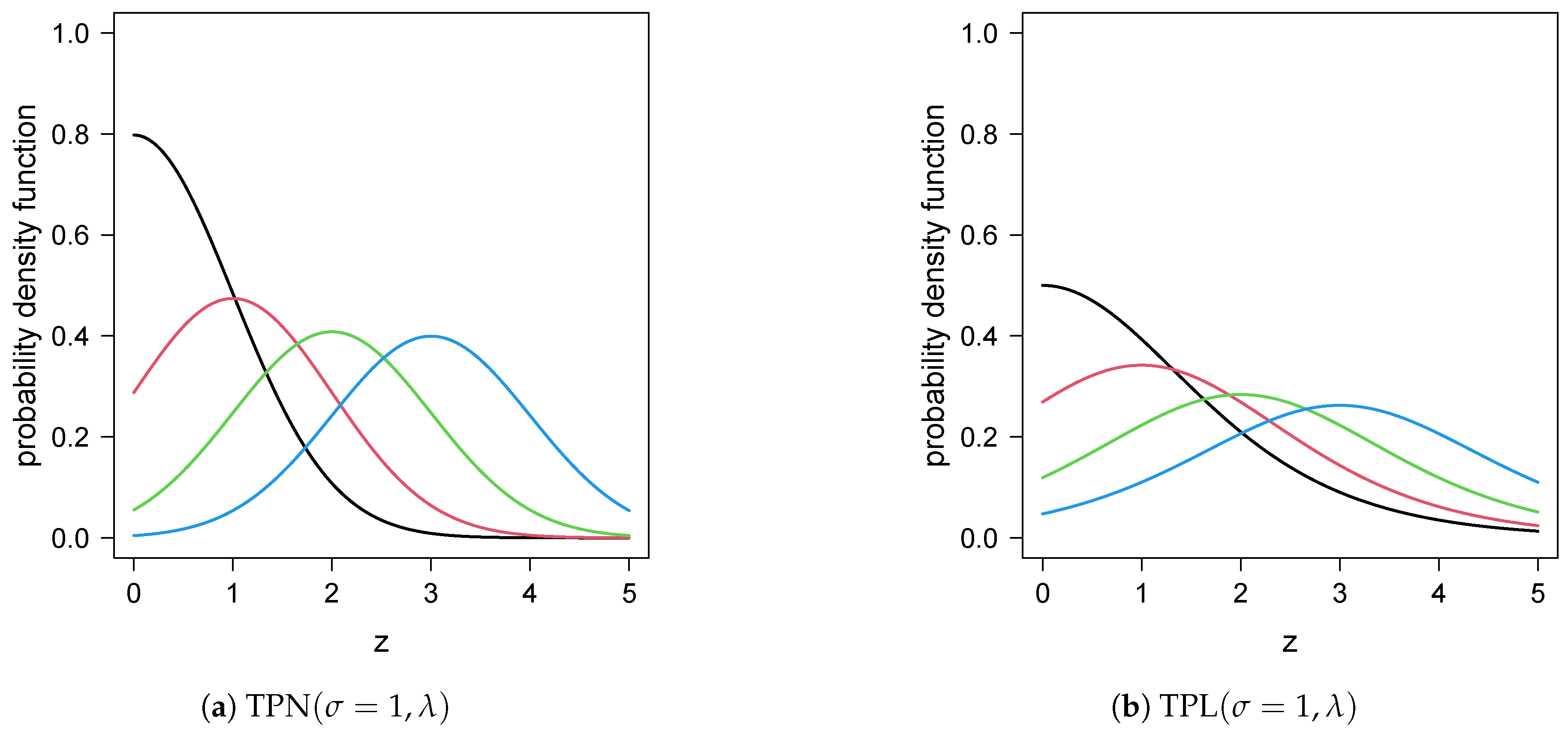
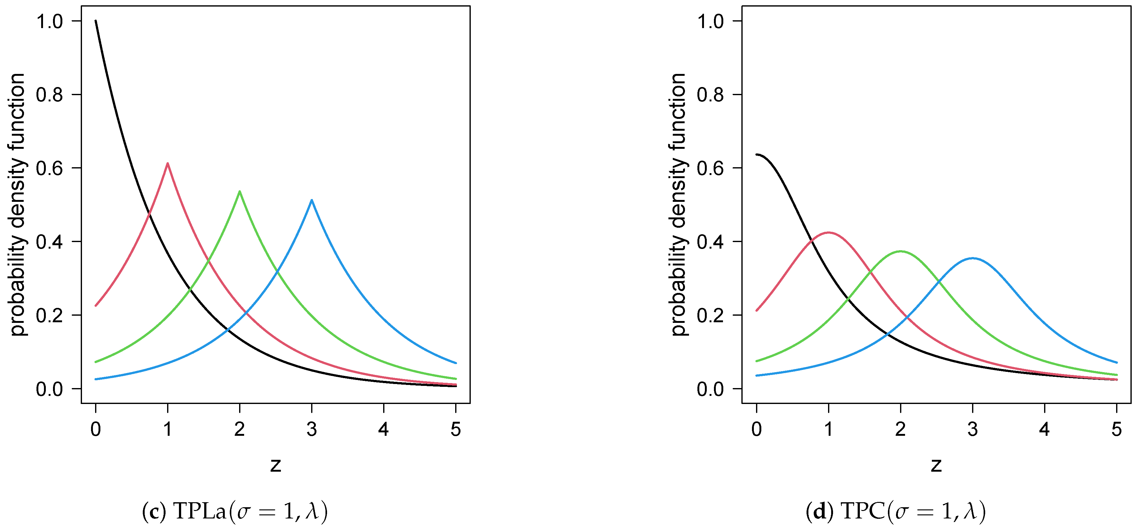
2. Truncated Positive Symmetrical Distributions
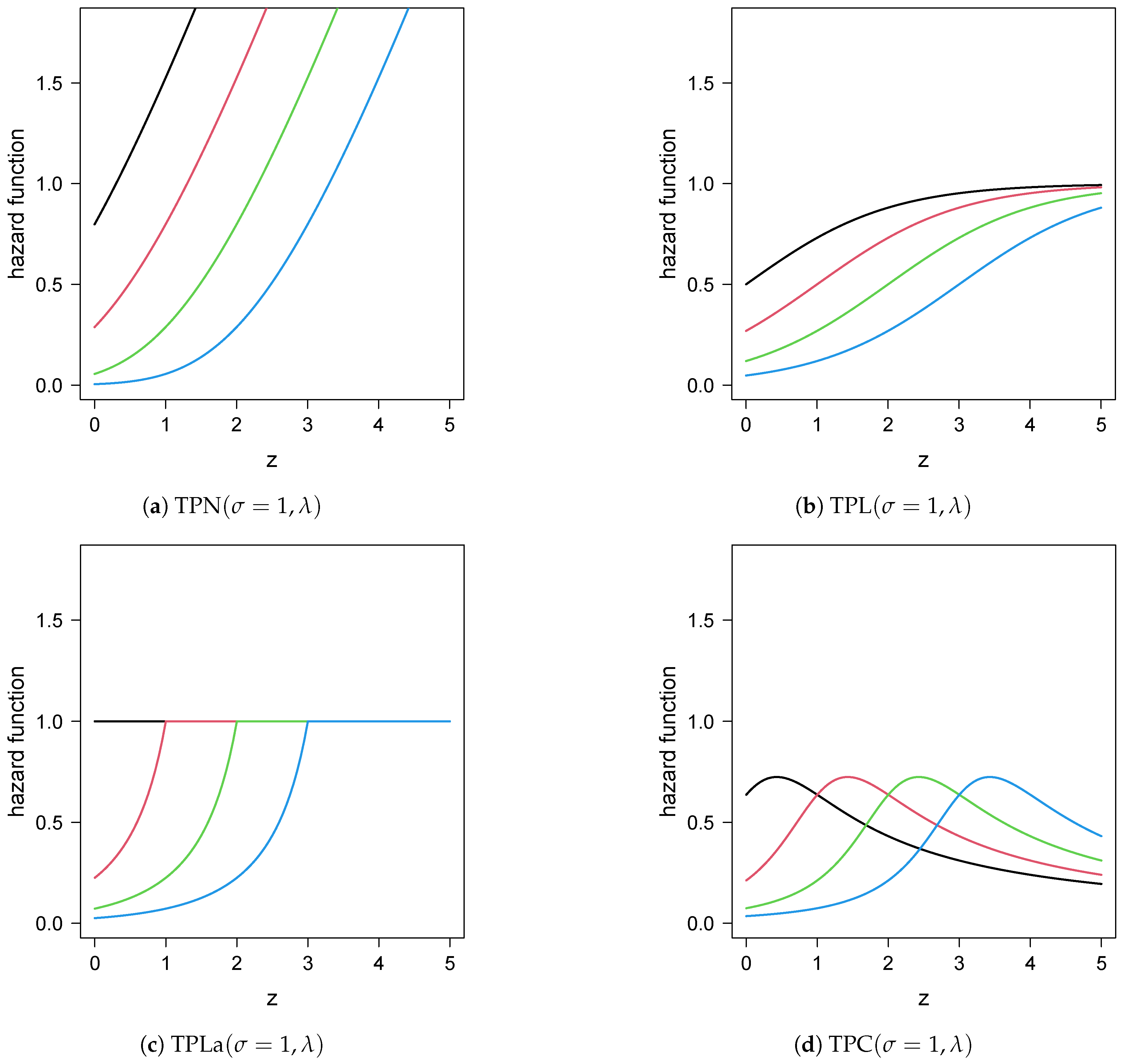
2.1. pdf, cdf and Hazard Function
2.2. Particular Cases
- ;
- ;
- ;
- ;
- .
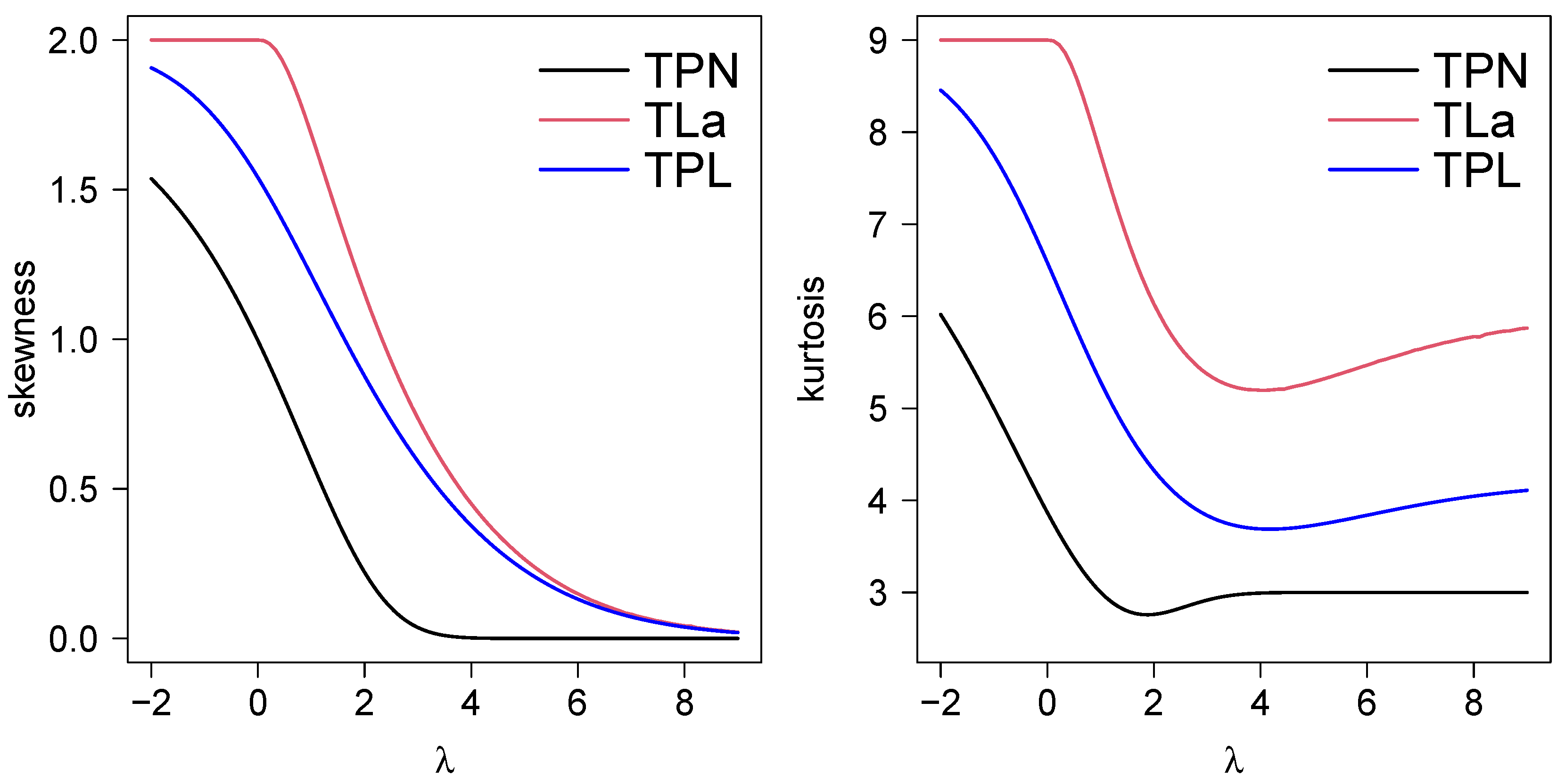
2.3. Moments
2.4. Shannon Entropy
2.5. Quantiles
- 1.
- First quartile: ;
- 2.
- Median: ;
- 3.
- Third quartile: .
2.6. Mode
- 1.
- when ;
- 2.
- when ,
2.7. Order Statistics
- 1.
- Minimum ().
- 2.
- Maximum ().
3. Inference
3.1. Moment Estimators
3.2. Maximum Likelihood Estimation
3.3. Observed Fisher Information Matrix
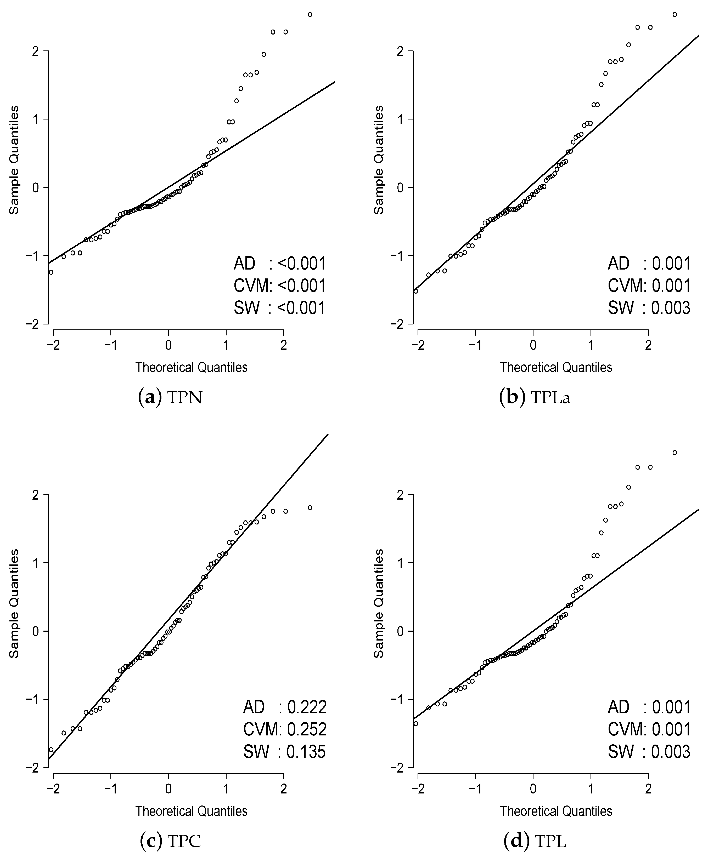
3.4. Residuals
3.5. Software
4. Simulation
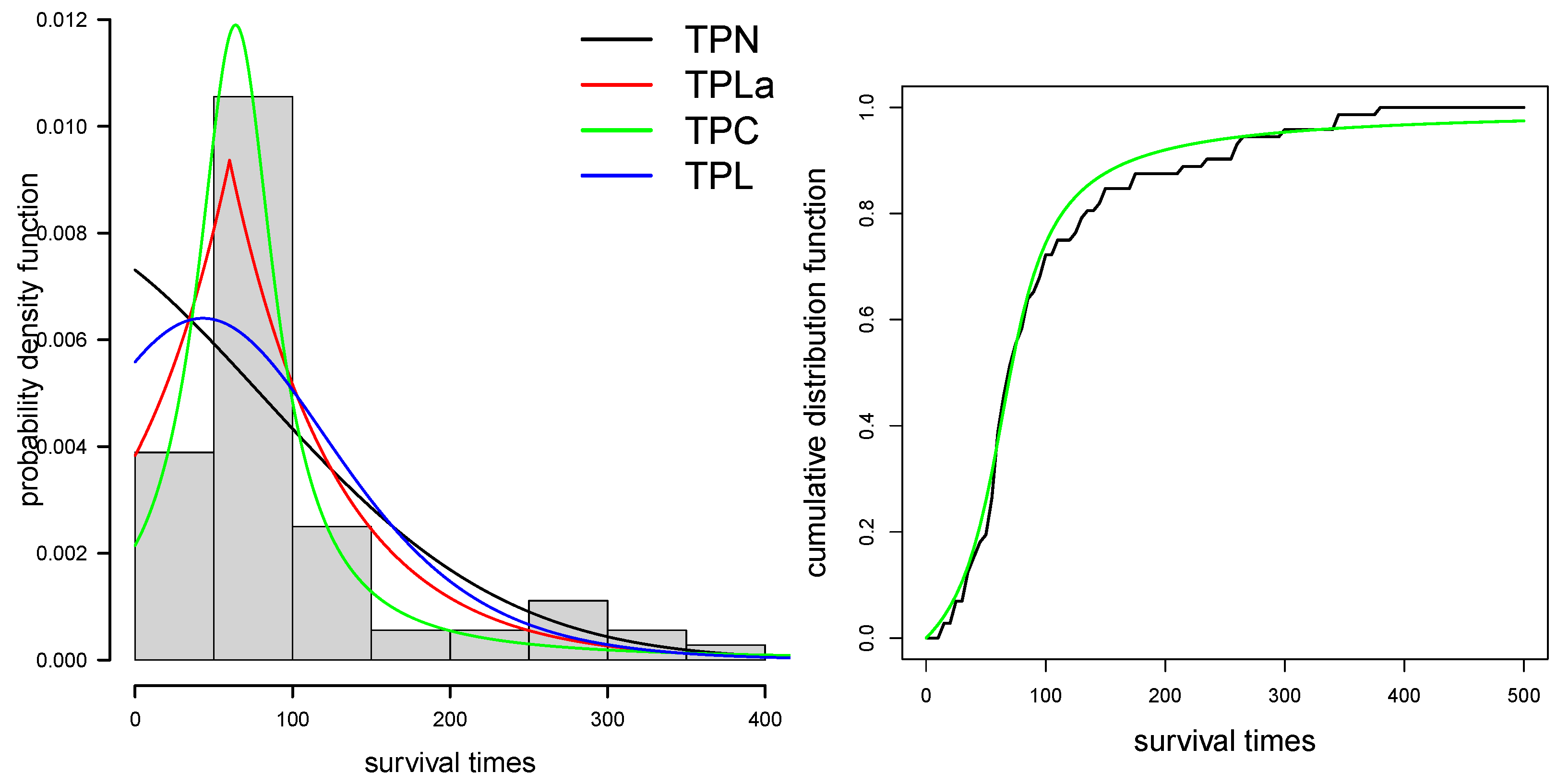
5. Application to Real Data
6. Conclusions
- The TPS family of distributions has turned out to be more flexible than the HS family, since it has a shape parameter;
- The TPS family of distributions is based on the univariate symmetric family of distributions. It has been proven that its properties are manageable and depend to a large extent on the properties of the pdf and cdf of the basal symmetric distribution;
- pdf, cdf and risk functions are represented by very well-known functions;
- A simulation study was carried out for some members of the TPS family. The ML estimators showed good performance for moderate sample sizes;
- A real application is given, in which several members of the TPS family were considered and fitted. The AIC and BIC model selection criteria showed which member had the best fit to this dataset. The AD, CVM and SW tests were carried out to validate the normality of the QR;
- As for the applicability of our results, we highlight that our proposal allowed us to incorporate a variety of shapes for modeling positive data, as has been established in Section 2. Therefore, these models can be considered as competitors to those commonly used for modeling lifetime data and other disciplines with positive data. On the other hand, an important advantage is that the new models inherit theoretical properties from the base models on which they are built, which increases their interest from an applied point of view;
- Practitioners may use the R package tpn for modeling positive continuous data.
Author Contributions
Funding
Institutional Review Board Statement
Informed Consent Statement
Data Availability Statement
Conflicts of Interest
References
- Kelker, D. Distribution theory of special distributions and location-scale parameter. Sankhya A 1970, 32, 419–430. [Google Scholar]
- Cambanis, S.; Huang, S.; Simons, G. On the theory of elliptically contoured distributions. J. Multivar. Anal. 1981, 11, 368–385. [Google Scholar] [CrossRef]
- Fang, K.T.; Kotz, S.; Ng, K.W. Symmetric Multivariate and Related Distributions; Chapman & Hall: London, UK; New York, NY, USA, 1990. [Google Scholar]
- Gupta, A.K.; Varga, T. Elliptically Contoured Models in Statistics; Kluwer Academics Publishers: Boston, MA, USA, 1993. [Google Scholar]
- Pewsey, A. Large-sample inference for the general half-normal distribution. Commun. Stat.-Theory Methods 2002, 31, 1045–1054. [Google Scholar] [CrossRef]
- Pewsey, A. Improved likelihood based inference for the general half-normal distribution. Commun. Stat.-Theory Methods 2004, 33, 197–204. [Google Scholar] [CrossRef]
- Chou, C.Y.; Liu, H.R. Properties of the half-normal distribution and its application to quality control. J. Ind. Technol. 1998, 14, 4–7. [Google Scholar]
- Barranco-Chamorro, I.; Moreno-Rebollo, J.L.; Pascual-Acosta, A.; Enguix-Gonzalez, A. An overview of asymptotic properties of estimator in truncated distributions. Commun. Stat.-Theory Methods 2007, 36, 2351–2366. [Google Scholar] [CrossRef]
- Cooray, K.; Ananda, M.M.A. A generalization of the half-normal distribution with applications to lifetime data. Commun. Stat.-Theory Methods 2008, 37, 1323–1337. [Google Scholar] [CrossRef]
- Olmos, N.M.; Varela, H.; Gómez, H.W.; Bolfarine, H. An extension of the half-normal distribution. Stat. Pap. 2012, 53, 875–886. [Google Scholar] [CrossRef]
- Balakrishnan, N.; Puthenpura, S. Best Linear Unbiased Estimators of Location and Scale Parameters of the Half Logistic Distribution. J. Stat. Comput. Simul. 1986, 25, 193–204. [Google Scholar] [CrossRef]
- Wiper, M.P.; Giron, F.J.; Pewsey, A. Objective Bayesian inference for the half-normal and half-t distributions. Commun. Stat.-Theory Methods 2008, 37, 3165–3185. [Google Scholar] [CrossRef]
- Polson, N.G.; Scott, J.G. On the half-Cauchy prior for a global scale parameter. Bayesian Anal. 2012, 7, 887–902. [Google Scholar] [CrossRef]
- Gui, W. Statistical Inferences and Applications of the Half Exponential Power Distribution. J. Qual. Reliab. Eng. 2013, 2013, 219473. [Google Scholar] [CrossRef]
- Almarashi, A.M.; Elgarhy, M.; Jamal, F.; Chesneau, C. The Exponentiated Truncated Inverse Weibull-Generated Family of Distributions with Applications. Symmetry 2020, 12, 650. [Google Scholar] [CrossRef]
- Bantan, R.A.R.; Chesneau, C.; Jamal, F.; Elbatal, I.; Elgarhy, M. The Truncated Burr X-G Family of Distributions: Properties and Applications to Actuarial and Financial Data. Entropy 2021, 23, 1088. [Google Scholar] [CrossRef] [PubMed]
- Morán-Vásquez, R.A.; Cataño Salazar, D.H.; Nagar, D.K. Some Results on the Truncated Multivariate Skew-Normal Distribution. Symmetry 2022, 14, 970. [Google Scholar] [CrossRef]
- Alotaibi, N.; Elbatal, I.; Almetwally, E.M.; Alyami, S.A.; Al-Moisheer, A.S.; Elgarhy, M. Truncated Cauchy Power Weibull-G Class of Distributions: Bayesian and Non-Bayesian Inference Modelling for COVID-19 and Carbon Fiber Data. Mathematics 2022, 10, 1565. [Google Scholar] [CrossRef]
- Gómez, H.J.; Olmos, N.M.; Varela, H.; Bolfarine, H. Inference for a truncated positive normal distribution. Appl. Math. J. Chin. Univ. 2018, 33, 163–176. [Google Scholar] [CrossRef]
- R Core Team. R: A Language and Environment for Statistical Computing; R Foundation for Statistical Computing: Vienna, Austria, 2023; Available online: https://www.R-project.org/ (accessed on 18 October 2023).
- Shannon, C.E. A Mathematical Theory of Communication. Bell Syst. Tech. J. 1948, 27, 379–423. [Google Scholar] [CrossRef]
- Balakrishnan, N.; Clifford Cohen, A. Order Statistics and Inference: Estimation Methods; Statistical Modeling and Decision Science Series; Elsevier Science: Amsterdam, The Netherlands, 1991. [Google Scholar]
- Dunn, P.K.; Smyth, G.K. Randomized Quantile Residuals. J. Comput. Graph. Stat. 1996, 5, 236–244. [Google Scholar]
- Gallardo, D.I.; Gómez, H.J.; Gómez, Y.M. tpn: Truncated Positive Normal Model and Extensions. R Package Version 1.7. 2023. Available online: https://CRAN.R-project.org/package=tpn (accessed on 18 October 2023).
- Bjerkedal, T. Acquisition of resistance in guinea pigs infected with different doses of virulent tubercle bacilli. Amer. J. Hyg. 1960, 72, 130–148. [Google Scholar] [PubMed]


| cdf | Hazard Function | ||
|---|---|---|---|
| Normal | |||
| Logistic | |||
| Laplace | |||
| Cauchy |
| TPN | TPL | TPLa | ||||
|---|---|---|---|---|---|---|
| −5 | 1.83 | 7.76 | 1.99 | 8.97 | 2.00 | 9.00 |
| −2 | 1.54 | 6.02 | 1.91 | 8.46 | 2.00 | 9.00 |
| −1 | 1.32 | 4.99 | 1.77 | 7.74 | 2.00 | 9.00 |
| 0 | 0.99 | 3.87 | 1.54 | 6.58 | 2.00 | 9.00 |
| 1 | 0.59 | 3.00 | 1.21 | 5.28 | 1.69 | 7.76 |
| 2 | 0.22 | 2.76 | 0.88 | 4.32 | 1.15 | 6.13 |
| 5 | 0.00 | 2.99 | 0.23 | 3.73 | 0.26 | 5.29 |
| True Values | |||||||||||||||
|---|---|---|---|---|---|---|---|---|---|---|---|---|---|---|---|
| Model | Estimator | Bias | SE | RMSE | CP | Bias | SE | RMSE | CP | Bias | SE | RMSE | CP | ||
| logistic | 1 | 0.5 | −0.010 | 0.210 | 0.213 | 0.897 | −0.003 | 0.150 | 0.151 | 0.922 | 0.000 | 0.107 | 0.109 | 0.940 | |
| −0.059 | 1.338 | 1.129 | 0.938 | 0.004 | 0.622 | 0.623 | 0.945 | −0.005 | 0.395 | 0.396 | 0.961 | ||||
| 1 | −0.005 | 0.197 | 0.196 | 0.919 | −0.004 | 0.138 | 0.138 | 0.934 | −0.002 | 0.098 | 0.097 | 0.943 | |||
| 0.017 | 0.760 | 0.751 | 0.958 | 0.022 | 0.475 | 0.480 | 0.959 | 0.011 | 0.330 | 0.329 | 0.955 | ||||
| 2 | −0.006 | 0.167 | 0.168 | 0.925 | 0.001 | 0.118 | 0.118 | 0.941 | −0.002 | 0.083 | 0.084 | 0.943 | |||
| 0.068 | 0.577 | 0.594 | 0.956 | 0.021 | 0.403 | 0.403 | 0.958 | 0.018 | 0.283 | 0.288 | 0.951 | ||||
| 3 | −0.009 | 0.145 | 0.149 | 0.925 | −0.005 | 0.102 | 0.104 | 0.933 | −0.002 | 0.073 | 0.074 | 0.944 | |||
| 0.091 | 0.577 | 0.595 | 0.950 | 0.050 | 0.404 | 0.409 | 0.949 | 0.024 | 0.284 | 0.288 | 0.949 | ||||
| 10 | 0.5 | −0.075 | 2.110 | 2.105 | 0.905 | −0.024 | 1.504 | 1.505 | 0.928 | −0.008 | 1.064 | 1.078 | 0.934 | ||
| −0.049 | 1.186 | 1.058 | 0.944 | 0.002 | 0.608 | 0.611 | 0.952 | −0.001 | 0.394 | 0.405 | 0.953 | ||||
| 1 | −0.015 | 1.978 | 2.060 | 0.912 | 0.003 | 1.392 | 1.416 | 0.934 | −0.029 | 0.977 | 0.993 | 0.936 | |||
| 0.029 | 0.746 | 0.764 | 0.950 | 0.013 | 0.476 | 0.482 | 0.959 | 0.007 | 0.330 | 0.333 | 0.955 | ||||
| 2 | −0.040 | 1.670 | 1.695 | 0.923 | −0.027 | 1.175 | 1.171 | 0.942 | −0.010 | 0.830 | 0.842 | 0.944 | |||
| 0.060 | 0.577 | 0.585 | 0.961 | 0.030 | 0.403 | 0.404 | 0.956 | 0.017 | 0.283 | 0.286 | 0.954 | ||||
| 3 | −0.053 | 1.457 | 1.466 | 0.929 | −0.024 | 1.029 | 1.011 | 0.946 | −0.010 | 0.727 | 0.720 | 0.944 | |||
| 0.084 | 0.577 | 0.601 | 0.956 | 0.039 | 0.404 | 0.400 | 0.953 | 0.018 | 0.284 | 0.281 | 0.954 | ||||
| Cauchy | 1 | 0.5 | −0.032 | 0.219 | 0.213 | 0.924 | −0.014 | 0.150 | 0.149 | 0.940 | −0.014 | 0.105 | 0.108 | 0.933 | |
| 0.028 | 0.506 | 0.523 | 0.977 | 0.007 | 0.322 | 0.551 | 0.974 | 0.029 | 0.176 | 0.176 | 0.956 | ||||
| 1 | −0.010 | 0.220 | 0.225 | 0.918 | −0.004 | 0.156 | 0.155 | 0.936 | −0.006 | 0.110 | 0.111 | 0.941 | |||
| 0.072 | 0.390 | 0.404 | 0.969 | 0.033 | 0.264 | 0.267 | 0.960 | 0.024 | 0.184 | 0.185 | 0.956 | ||||
| 2 | 0.000 | 0.219 | 0.227 | 0.929 | −0.002 | 0.154 | 0.155 | 0.938 | −0.002 | 0.109 | 0.109 | 0.942 | |||
| 0.104 | 0.527 | 0.552 | 0.954 | 0.052 | 0.364 | 0.375 | 0.952 | 0.029 | 0.254 | 0.257 | 0.952 | ||||
| 3 | −0.002 | 0.214 | 0.221 | 0.929 | 0.000 | 0.151 | 0.153 | 0.940 | −0.003 | 0.106 | 0.105 | 0.945 | |||
| 0.153 | 0.716 | 0.750 | 0.950 | 0.070 | 0.492 | 0.503 | 0.950 | 0.043 | 0.344 | 0.340 | 0.957 | ||||
| 10 | 0.5 | −0.345 | 2.203 | 2.167 | 0.914 | −0.088 | 1.502 | 1.498 | 0.940 | −0.149 | 1.052 | 1.047 | 0.943 | ||
| 0.032 | 0.499 | 0.518 | 0.975 | 0.002 | 0.366 | 0.549 | 0.978 | 0.031 | 0.175 | 0.175 | 0.965 | ||||
| 1 | −0.134 | 2.184 | 2.207 | 0.923 | −0.071 | 1.560 | 1.576 | 0.930 | −0.083 | 1.100 | 1.095 | 0.944 | |||
| 0.071 | 0.384 | 0.392 | 0.975 | 0.030 | 0.326 | 0.532 | 0.959 | 0.027 | 0.184 | 0.184 | 0.959 | ||||
| 2 | −0.048 | 2.176 | 2.172 | 0.925 | −0.003 | 1.544 | 1.556 | 0.940 | −0.015 | 1.087 | 1.079 | 0.944 | |||
| 0.112 | 0.528 | 0.548 | 0.959 | 0.050 | 0.364 | 0.371 | 0.953 | 0.027 | 0.254 | 0.254 | 0.958 | ||||
| 3 | −0.009 | 2.149 | 2.218 | 0.928 | −0.004 | 1.507 | 1.540 | 0.939 | −0.018 | 1.062 | 1.079 | 0.941 | |||
| 0.149 | 0.717 | 0.751 | 0.953 | 0.074 | 0.492 | 0.502 | 0.952 | 0.041 | 0.344 | 0.353 | 0.944 | ||||
| Dataset | n | ||||
|---|---|---|---|---|---|
| Survival Times of Guinea Pigs in Days | 72 |
| Parameters | TPN | TPLa | TPC | TPL |
|---|---|---|---|---|
| 154.944 (47.298) | 67.772 (0.035) | 29.926 (5.895) | 57.513 (10.091) | |
| −0.488 (0.762) | 0.885 (0.004) | 2.133 (0.451) | 0.749 (0.556) | |
| log-likelihood | −401.46 | −392.27 | −391.16 | −399.38 |
| AIC | 806.92 | 788.54 | 786.33 | 802.75 |
| BIC | 811.47 | 793.09 | 790.88 | 807.31 |
| KS (p-value) | 0.152 (0.073) | 0.105 (0.400) | 0.085 (0.675) | 0.126 (0.200) |
Disclaimer/Publisher’s Note: The statements, opinions and data contained in all publications are solely those of the individual author(s) and contributor(s) and not of MDPI and/or the editor(s). MDPI and/or the editor(s) disclaim responsibility for any injury to people or property resulting from any ideas, methods, instructions or products referred to in the content. |
© 2023 by the authors. Licensee MDPI, Basel, Switzerland. This article is an open access article distributed under the terms and conditions of the Creative Commons Attribution (CC BY) license (https://creativecommons.org/licenses/by/4.0/).
Share and Cite
Gómez, H.J.; Santoro, K.I.; Barranco-Chamorro, I.; Venegas, O.; Gallardo, D.I.; Gómez, H.W. A Family of Truncated Positive Distributions. Mathematics 2023, 11, 4431. https://doi.org/10.3390/math11214431
Gómez HJ, Santoro KI, Barranco-Chamorro I, Venegas O, Gallardo DI, Gómez HW. A Family of Truncated Positive Distributions. Mathematics. 2023; 11(21):4431. https://doi.org/10.3390/math11214431
Chicago/Turabian StyleGómez, Héctor J., Karol I. Santoro, Inmaculada Barranco-Chamorro, Osvaldo Venegas, Diego I. Gallardo, and Héctor W. Gómez. 2023. "A Family of Truncated Positive Distributions" Mathematics 11, no. 21: 4431. https://doi.org/10.3390/math11214431
APA StyleGómez, H. J., Santoro, K. I., Barranco-Chamorro, I., Venegas, O., Gallardo, D. I., & Gómez, H. W. (2023). A Family of Truncated Positive Distributions. Mathematics, 11(21), 4431. https://doi.org/10.3390/math11214431