
Testing Equality of Several Distributions at High Dimensions: A Maximum-Mean-Discrepancy-Based Approach


Abstract
:1. Introduction
2. Main Results
2.1. MMD for Several Distributions
2.2. Computation of the Test Statistic
2.3. Asymptotic Null Distribution
- C1.
- We have .
- C2.
- As , we have .
- C3.
- is a reproduced kernel such that .
2.4. Mean and Variance of
2.5. Asymptotic Power
3. Methods for Implementing the Proposed Test
3.1. Parametric Bootstrap Method
3.2. Random Permutation Method
3.3. Welch–Satterthwaite -Approximation Method
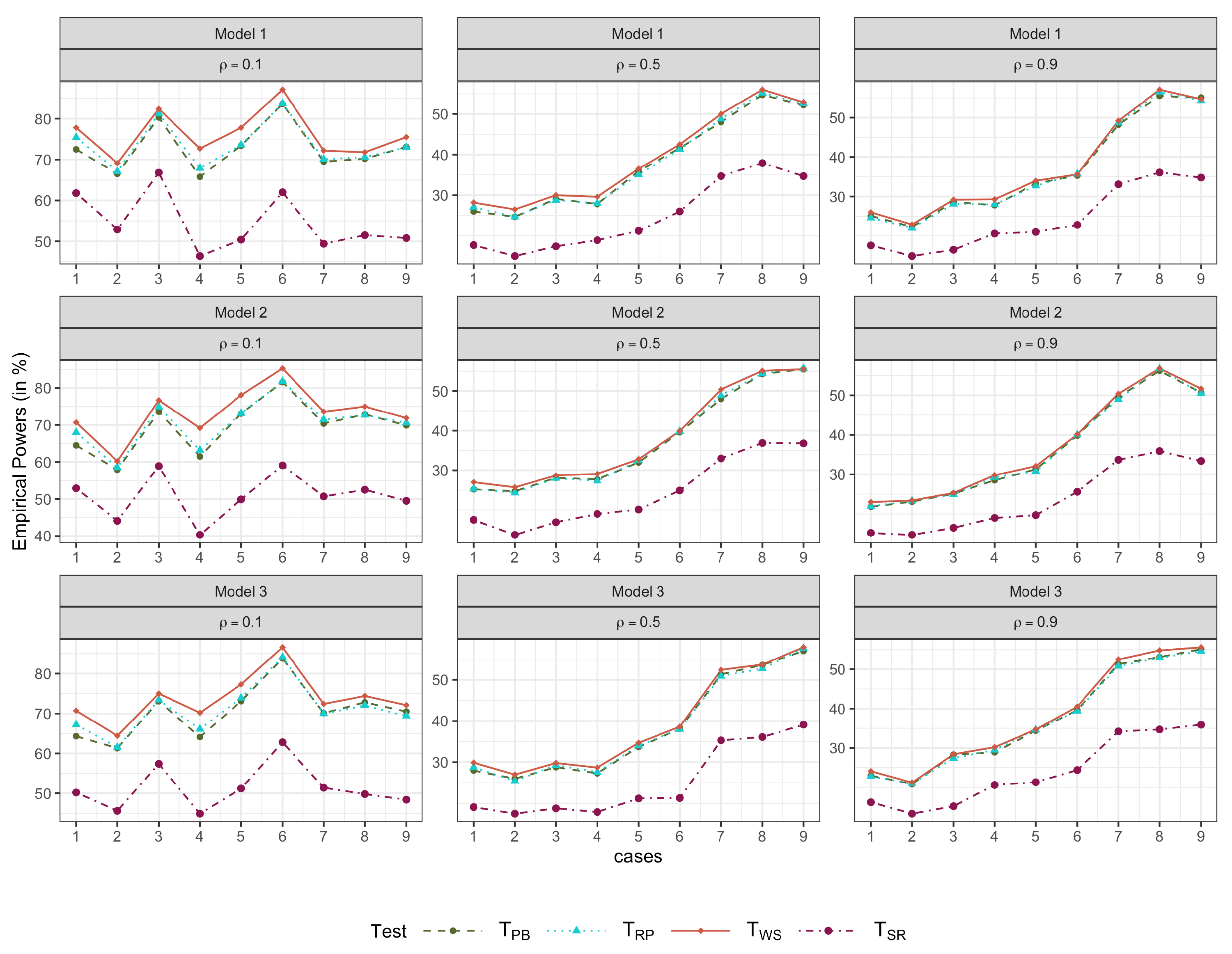
4. Simulation Studies
4.1. Simulation 1
- Model 1.
- .
- Model 2.
- with ; .
- Model 3.
- with .
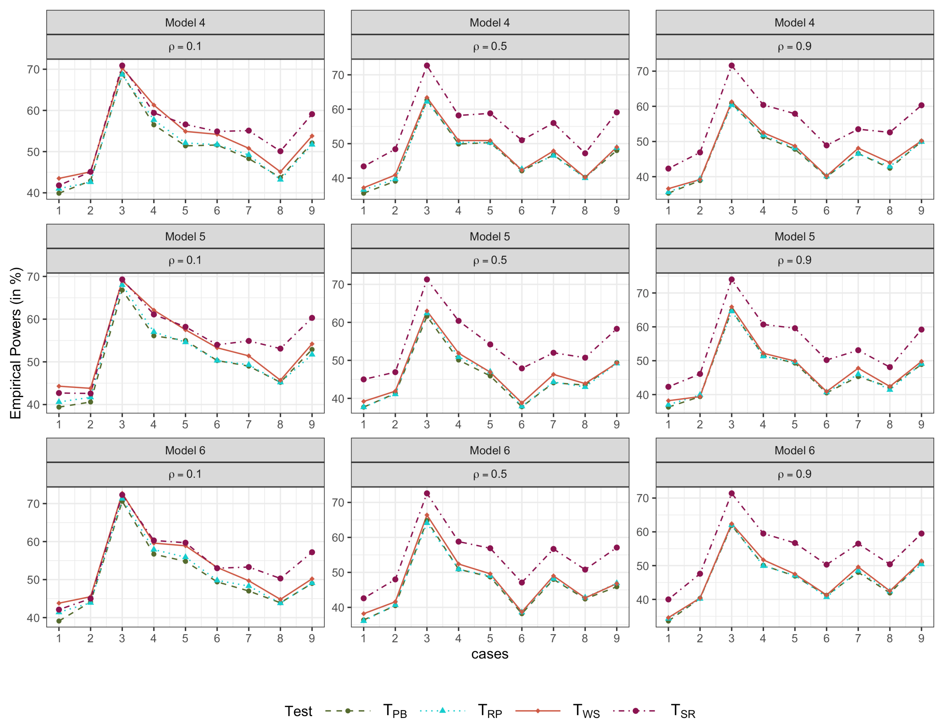
4.2. Simulation 2
- Model 4.
- .
- Model 5.
- with .
- Model 6.
- with , .
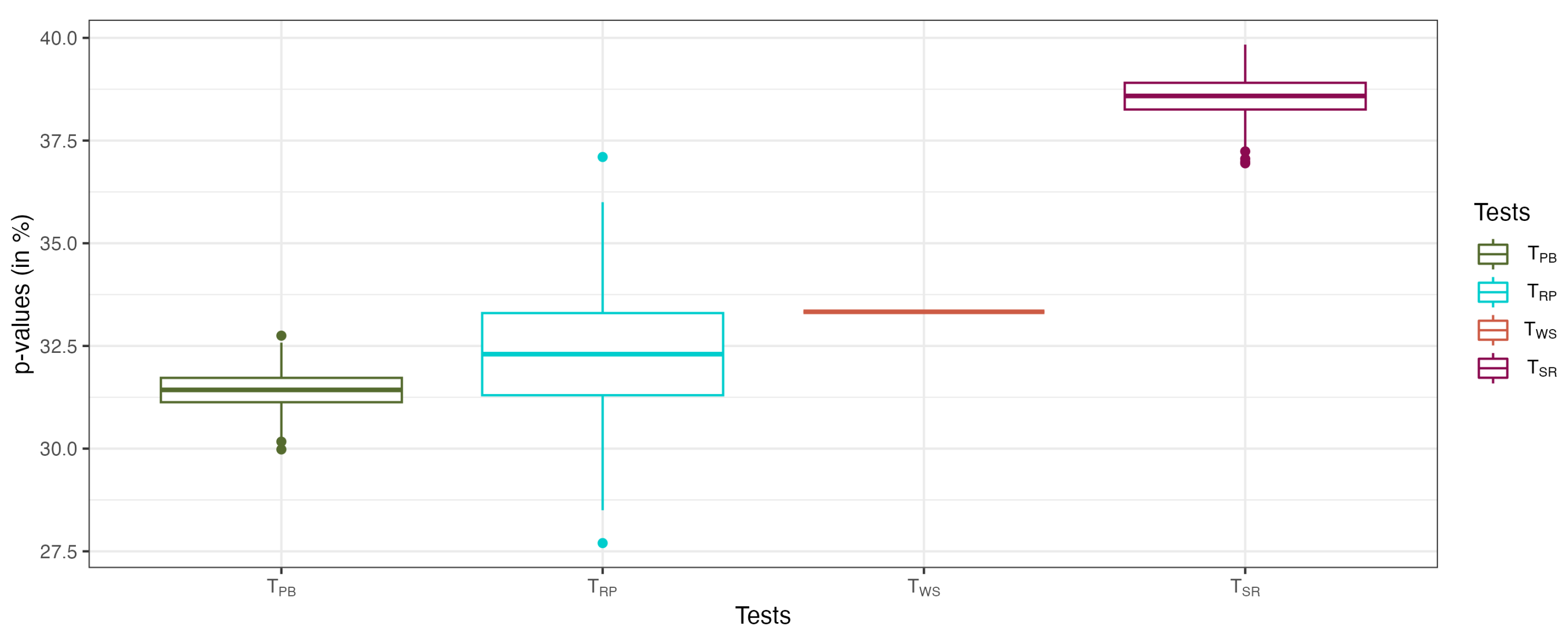
5. Application to the Corneal Surface Data
6. Concluding Remarks
Author Contributions
Funding
Data Availability Statement
Conflicts of Interest
Abbreviations
| MMD | Maximum Mean Discrepancy |
| EDF | Empirical Distribution Function |
| RKHS | Reproducing Kernel Hilbert Spaces |
| RBF | Radial Basis Function |
| ARE | Average Relative Error |
Appendix A. Technical Proofs
References
- Lehmann, E.L. Nonparametrics: Statistical Methods Based on Ranks; Springer: New York, NY, USA, 2006. [Google Scholar]
- Friedman, J.H.; Rafsky, L.C. Multivariate Generalizations of the Wald–Wolfowitz and Smirnov Two-Sample Tests. Ann. Stat. 1979, 7, 697–717. [Google Scholar] [CrossRef]
- Schilling, M.F. Multivariate Two-Sample Tests Based on Nearest Neighbors. J. Am. Stat. Assoc. 1986, 81, 799–806. [Google Scholar] [CrossRef]
- Baringhaus, L.; Franz, C. On a new multivariate two-sample test. J. Multivar. Anal. 2004, 88, 190–206. [Google Scholar] [CrossRef]
- Rosenbaum, P.R. An exact distribution-free test comparing two multivariate distributions based on adjacency. J. R. Stat. Soc. Ser. B 2005, 67, 515–530. [Google Scholar] [CrossRef]
- Biswas, M.; Mukhopadhyay, M.; Ghosh, A.K. A distribution-free two-sample run test applicable to high-dimensional data. Biometrika 2014, 101, 913–926. [Google Scholar] [CrossRef]
- Li, J. Asymptotic normality of interpoint distances for high-dimensional data with applications to the two-sample problem. Biometrika 2018, 105, 529–546. [Google Scholar] [CrossRef]
- Chen, H.; Friedman, J.H. A New Graph-Based Two-Sample Test for Multivariate and Object Data. J. Am. Stat. Assoc. 2017, 112, 397–409. [Google Scholar] [CrossRef]
- Hall, P.; Tajvidi, N. Permutation Tests for Equality of Distributions in High-Dimensional Settings. Biometrika 2002, 89, 359–374. [Google Scholar] [CrossRef]
- Wei, S.; Lee, C.; Wichers, L.; Marron, J.S. Direction-Projection-Permutation for High-Dimensional Hypothesis Tests. J. Comput. Graph. Stat. 2016, 25, 549–569. [Google Scholar] [CrossRef]
- Ghosh, A.K.; Biswas, M. Distribution-free high-dimensional two-sample tests based on discriminating hyperplanes. Test 2016, 25, 525–547. [Google Scholar] [CrossRef]
- Székely, G.J.; Rizzo, M.L. Testing for equal distributions in high dimension. InterStat 2004, 5, 1249–1272. [Google Scholar]
- Gretton, A.; Borgwardt, K.M.; Rasch, M.J.; Schölkopf, B.; Smola, A. A Kernel Two-Sample Test. J. Mach. Learn. Res. 2012, 13, 723–773. [Google Scholar]
- Sejdinovic, D.; Sriperumbudur, B.; Gretton, A.; Fukumizu, K. Equivalence of distance-based and RKHS-based statistics in hypothesis testing. Ann. Stat. 2013, 41, 2263–2291. [Google Scholar] [CrossRef]
- Zhang, J.T.; Smaga, Ł. Two-sample test for equal distributions in separable metric space: New maximum mean discrepancy based approaches. Electron. J. Stat. 2022, 16, 4090–4132. [Google Scholar] [CrossRef]
- Zhou, B.; Ong, Z.P.; Zhang, J.T. A new MMD-based two-sample test for equal distributions in separable metric spaces. Manuscript 2023, in press.
- Balogoun, A.S.K.; Nkiet, G.M.; Ogouyandjou, C. k-Sample problem based on generalized maximum mean discrepancy. arXiv 2018, arXiv:1811.09103. [Google Scholar]
- Zhang, J.T.; Guo, J.; Zhou, B. Testing equality of several distributions in separable metric spaces: A maximum mean discrepancy based approach. J. Econom. 2022, in press. [CrossRef]
- Zhang, J.T.; Guo, J.; Zhou, B. Linear hypothesis testing in high-dimensional one-way MANOVA. J. Multivar. Anal. 2017, 155, 200–216. [Google Scholar] [CrossRef]
- Gretton, A.; Fukumizu, K.; Harchaoui, Z.; Sriperumbudur, B.K. A Fast, Consistent Kernel Two-Sample Test. In Advances in Neural Information Processing Systems 22; Curran Associates, Inc.: New York, NY, USA, 2009; pp. 673–681. [Google Scholar]
- Welch, B.L. The generalization of `student’s’ problem when several different population variances are involved. Biometrika 1947, 34, 28–35. [Google Scholar] [CrossRef]
- Satterthwaite, F.E. An Approximate Distribution of Estimates of Variance Components. Biom. Bull. 1946, 2, 110–114. [Google Scholar] [CrossRef]
- Zhang, J.T. Two-Way MANOVA with Unequal Cell Sizes and Unequal Cell Covariance Matrices. Technometrics 2011, 53, 426–439. [Google Scholar] [CrossRef]
- Smaga, Ł.; Zhang, J.T. Linear Hypothesis Testing with Functional Data. Technometrics 2019, 61, 99–110. [Google Scholar] [CrossRef]

| Model | (n1, n2, n3) | |||||||||||||
|---|---|---|---|---|---|---|---|---|---|---|---|---|---|---|
| 4.0 | 4.5 | 5.2 | 4.9 | 4.4 | 4.0 | 4.7 | 4.1 | 5.7 | 5.5 | 6.1 | 5.9 | |||
| 10 | 4.9 | 5.0 | 5.6 | 5.3 | 5.8 | 5.7 | 6.0 | 5.2 | 4.2 | 4.1 | 4.3 | 4.8 | ||
| 5.1 | 5.1 | 5.2 | 4.9 | 4.0 | 4.2 | 4.4 | 3.9 | 4.6 | 5.4 | 4.9 | 4.3 | |||
| 4.8 | 5.2 | 6.5 | 4.8 | 4.2 | 4.6 | 4.3 | 4.7 | 5.9 | 5.6 | 6.1 | 5.9 | |||
| 1 | 100 | 4.6 | 4.4 | 4.9 | 3.9 | 4.8 | 5.1 | 5.3 | 5.3 | 5.1 | 5.3 | 5.3 | 5.5 | |
| 5.8 | 5.6 | 6.9 | 5.5 | 4.7 | 4.5 | 4.5 | 4.2 | 4.6 | 4.3 | 5.0 | 4.5 | |||
| 5.0 | 5.4 | 5.8 | 4.9 | 4.3 | 4.4 | 4.7 | 4.8 | 3.8 | 4.4 | 4.5 | 4.5 | |||
| 500 | 4.9 | 5.3 | 5.8 | 4.3 | 5.0 | 5.2 | 5.3 | 5.4 | 5.0 | 5.3 | 5.5 | 5.3 | ||
| 6.2 | 6.2 | 7.0 | 5.7 | 6.4 | 6.2 | 6.4 | 6.4 | 4.8 | 4.4 | 5.0 | 5.2 | |||
| 4.9 | 5.5 | 6.6 | 5.7 | 4.4 | 4.5 | 5.0 | 4.9 | 5.6 | 5.0 | 5.7 | 5.6 | |||
| 10 | 5.6 | 5.6 | 6.4 | 5.8 | 3.6 | 3.5 | 4.0 | 4.5 | 5.4 | 5.3 | 5.3 | 4.9 | ||
| 5.7 | 5.8 | 6.8 | 6.3 | 4.9 | 5.5 | 5.8 | 5.2 | 5.3 | 5.5 | 5.7 | 5.1 | |||
| 4.9 | 5.1 | 5.9 | 5.0 | 5.4 | 5.5 | 5.5 | 5.3 | 3.9 | 4.5 | 4.7 | 4.3 | |||
| 2 | 100 | 5.5 | 5.6 | 6.6 | 5.5 | 4.5 | 4.3 | 4.9 | 3.8 | 5.8 | 5.6 | 5.7 | 5.6 | |
| 5.1 | 5.3 | 5.6 | 4.9 | 6.4 | 6.5 | 6.8 | 7.0 | 5.0 | 4.8 | 4.8 | 4.1 | |||
| 5.0 | 5.1 | 5.4 | 5.5 | 5.9 | 5.8 | 6.0 | 6.6 | 5.0 | 5.2 | 5.3 | 5.5 | |||
| 500 | 4.8 | 4.3 | 5.4 | 5.2 | 5.7 | 5.6 | 5.7 | 5.1 | 4.1 | 3.9 | 4.0 | 3.9 | ||
| 4.2 | 4.3 | 5.0 | 4.9 | 4.6 | 4.4 | 4.8 | 4.4 | 5.4 | 5.7 | 5.4 | 5.9 | |||
| 4.2 | 5.0 | 5.6 | 4.8 | 5.4 | 6.0 | 6.5 | 5.7 | 4.9 | 4.9 | 5.5 | 4.8 | |||
| 10 | 4.9 | 5.0 | 5.5 | 4.9 | 4.9 | 4.4 | 5.0 | 5.0 | 5.2 | 5.1 | 5.4 | 5.4 | ||
| 4.5 | 4.6 | 5.5 | 4.9 | 5.0 | 5.0 | 5.4 | 5.0 | 6.0 | 5.9 | 5.8 | 5.8 | |||
| 4.1 | 4.4 | 5.1 | 4.7 | 5.0 | 5.5 | 5.8 | 4.5 | 5.0 | 5.0 | 5.4 | 4.4 | |||
| 3 | 100 | 3.1 | 3.5 | 4.0 | 4.5 | 4.8 | 5.2 | 5.0 | 4.4 | 5.0 | 5.0 | 5.0 | 5.0 | |
| 4.7 | 4.5 | 5.4 | 5.0 | 4.8 | 4.8 | 5.1 | 4.5 | 4.6 | 4.6 | 4.8 | 3.9 | |||
| 4.9 | 4.7 | 5.4 | 6.0 | 5.0 | 4.6 | 5.4 | 4.5 | 4.1 | 4.1 | 4.5 | 3.9 | |||
| 500 | 5.6 | 5.8 | 6.1 | 5.5 | 4.3 | 4.2 | 4.5 | 4.7 | 4.8 | 5.0 | 5.1 | 5.2 | ||
| 5.0 | 4.8 | 5.5 | 6.0 | 4.4 | 4.5 | 4.6 | 4.5 | 5.5 | 5.4 | 5.6 | 6.0 | |||
| ARE | 9.04 | 9.33 | 16.22 | 8.67 | 10.67 | 12.52 | 11.56 | 11.70 | 9.26 | 8.74 | 9.19 | 11.56 | ||
| Method | ||||
|---|---|---|---|---|
| Case | ||||
| NOR vs. UNI vs. SUS vs. CLI | 0 | 0 | 0.00004 | 0.09 |
| NOR vs. UNI vs. SUS | 31.2 | 32.3 | 33.3 | 38.9 |
| NOR vs. UNI vs. CLI | 0.02 | 0 | 0.0012 | 0.25 |
| NOR vs. SUS vs. CLI | 0 | 0 | 0.00001 | 0.01 |
| UNI vs. SUS vs. CLI | 0.01 | 0 | 0.0012 | 0.24 |
Disclaimer/Publisher’s Note: The statements, opinions and data contained in all publications are solely those of the individual author(s) and contributor(s) and not of MDPI and/or the editor(s). MDPI and/or the editor(s) disclaim responsibility for any injury to people or property resulting from any ideas, methods, instructions or products referred to in the content. |
© 2023 by the authors. Licensee MDPI, Basel, Switzerland. This article is an open access article distributed under the terms and conditions of the Creative Commons Attribution (CC BY) license (https://creativecommons.org/licenses/by/4.0/).
Share and Cite
Ong, Z.P.; Chen, A.A.; Zhu, T.; Zhang, J.-T. Testing Equality of Several Distributions at High Dimensions: A Maximum-Mean-Discrepancy-Based Approach. Mathematics 2023, 11, 4374. https://doi.org/10.3390/math11204374
Ong ZP, Chen AA, Zhu T, Zhang J-T. Testing Equality of Several Distributions at High Dimensions: A Maximum-Mean-Discrepancy-Based Approach. Mathematics. 2023; 11(20):4374. https://doi.org/10.3390/math11204374
Chicago/Turabian StyleOng, Zhi Peng, Aixiang Andy Chen, Tianming Zhu, and Jin-Ting Zhang. 2023. "Testing Equality of Several Distributions at High Dimensions: A Maximum-Mean-Discrepancy-Based Approach" Mathematics 11, no. 20: 4374. https://doi.org/10.3390/math11204374
APA StyleOng, Z. P., Chen, A. A., Zhu, T., & Zhang, J.-T. (2023). Testing Equality of Several Distributions at High Dimensions: A Maximum-Mean-Discrepancy-Based Approach. Mathematics, 11(20), 4374. https://doi.org/10.3390/math11204374