Abstract
This paper proposes a prey–predator model affected by fear effects and toxic substances. We used the Lipschitz condition to prove the uniqueness of the model solution and Laplace transform to prove the boundedness of the model solution. We used the fractional-order stability theorem to provide sufficient conditions for the local stability of equilibrium points, and selected fractional-order derivatives as parameters to perform Hopf bifurcation analysis on the system. Finally, the theoretical results are verified via numerical simulation. The results show that a value of will affect the stability of the system and that the population size and the effect of toxic substances have a huge impact on the stability of the system.
Keywords:
prey–predator model; fractional-order system; fear effect; toxic injections; Holling II functional response MSC:
92B05; 92C42
1. Introduction
Population dynamics have developed rapidly since the 18th century, and the complex interspecific relationships between different populations have been extensively studied [1,2,3,4,5]. Due to the good memory properties of fractional calculus, it can be applied to biological models to more closely mimic the evolution of biological populations in reality [6]. Fractional calculus also overcomes the issue that the theory of the classical integer-order differential model does not agree well with the experimental results, and fractional calculus only needs to use a few parameters to obtain better results [7,8].Fractional-order differential operators are effectively applied to numerical analysis tools in physics, mechanics, science, and mathematics. Compared to integer calculus, fractional calculus provides us with better discoveries than traditional models [9]. Ref. [10] investigated the solution of the fractional multidimensional Navier–Stokes equation based on the Caputo fractional derivative operator. In Ref. [11], the dynamic behavior of a fractional-order predator–prey model with prey shelters was studied. Therefore, this paper will study the fractional prey–predator model.
With the development of population dynamics, complex interspecific relationships among different populations have been extensively studied, and various external factors affecting biological populations have also received extensive attention. Field experiments have raised awareness that fear effects have important implications for prey–predator models [12]. Fear effects are common in the natural environment and have important impacts on populations, but they are often overlooked in conservation or wildlife management. The indirect effects of predators on prey lead to physiological and behavioral changes in the prey species, such as reduced foraging activity, increased vigilance, and changes in habitat utilization, resulting in a decrease in the number of prey animals. Some studies have shown that the indirect effects of predators may cause hormonal changes in prey [13]. The fear effect has different effects on different species [14,15], such as moving to other places to live, affecting their foraging behavior, affecting their reproduction, etc. In [16], the author showed through experiments that the fear effect reduced the offspring of song sparrows by . Ref. [17] has shown that the fear effect causes female guppies to shorten the retention time of their pups, potentially producing offspring with impaired motility. Ref. [18] studied the model of how the fear effect affects the biological reproduction rate, explored the relationship between the fear effect and other biologically relevant parameters, and further demonstrated the effect of fear on the prey–predator model. Ref. [19] studied a class of prey–predator models affected by infectious diseases, in which the prey is susceptible and will be affected by the fear effect, and the results show that the density of infected prey is proportional to the degree of fear caused by the predator. Ref. [20] studied a class of biological models affected by both the fear effect and the group defense effect, and the results showed that an excessive fear effect may lead to the extinction of prey species. Ref. [21] proposed a class of prey–predator models with prey shelter and affected by fear effects, and studied its equilibrium and bifurcation problems. In [22], the authors considered a biological model with two predators with hunting cooperation, and the effect of fear on the prey was considered. A biological model with multiple Allee effects caused by fear effects was considered in [23].
In today’s global trend of industrialization, various factories emit toxic gases and hazardous wastes containing a large amount of toxic heavy metals, which seriously pollute the natural environment and destroy the living environment of wild animals [24,25]. The destruction of the environment by toxic substances has caused many wild animals to be harmed; some species have become extinct, and the number of many organisms has dropped sharply due to these toxic substances. Ref. [26] found that toxic substances can be delivered directly to organisms or through the food chain by consuming prey, delivering toxic substances to predators. In [27], the authors looked at the problem of fishing between two competing fish species, both of which release toxic substances that are harmful to the other. Ref. [28] studied populations of organisms living in polluted environments for a long time and derived the conditions for the persistence of populations. Ref. [29] studied a class of prey–predator models with fear effects under toxic substances, in which the prey is directly affected by the toxic substance, while the predator is affected by consuming the prey; the authors studied the non-negative solution of this system, as well as its nature, boundedness, and consistency continuity, and give the conditions for the extinction of prey and predators and the conditions for the continued existence of the system.
In this paper, a predator–prey system affected by fear effects and toxic substances was considered, combined with the dual effects of environmental pollution and fear effects in recent years, which is more in line with the real biological chain. The main results are as follows. Firstly, the uniqueness and boundedness of the solutions of the system are studied. Secondly, the equilibrium point of the model is given, and the sufficient conditions for the local stability of the equilibrium point are given by the fractional stability theorem. Thirdly, the Hopf bifurcation at the equilibrium point of the system is analyzed.
The rest of this paper is organized as follows. In Section 2, we introduce models influenced by fear effects and toxic substances and provide some definitions and lemmas required for this paper. In Section 3, we investigate the uniqueness, boundedness, and local stability of the model. The Hopf bifurcation at the equilibrium point is analyzed.
2. Model Description and Preliminaries
In this section, the prey–predator system affected by fear effects and toxic substances is presented, and the basic knowledge and lemmas needed for this paper are presented as well. In the whole paper, Caputo fractional derivatives [30] are used in the model.
Lemma 1
([31]). Suppose , , are non-decreasing, non-negative, and locally integrable functions; is a non-negative, locally integrable function; and and satisfies
then,
where
Lemma 2
([32]). For system
where function : and , if
the equilibrium point of system (1) is locally asymptotically stable, where are the eigenvalues of the system.
Lemma 3
([33]). For system
the sufficient condition for system (2) to have a unique solution is that satisfies the local Lipschitz for h on .
In general, in the absence of predator and fear effects, herbivore growth is determined by natural mortality, density-dependent mortality, and reproduction rates [19]:
where x is the density of the prey population, r is the reproductive rate, c is the density-dependent mortality, and d is the natural mortality.
From [16], it can be seen that the fear effect will affect the reproduction rate of the population. Therefore, we multiply the reproduction rate by a fear factor (proposed by [18], where is the fear level of the prey). This equation can be expressed as:
where y represents the population density of predators, and is the fear function, which has the following properties:
Therefore, this paper propose a prey–predator model with fear effects and Holling II-type function responses:
where is the predation coefficient, is the food conversion coefficient, b is the half-saturation constant, is the natural mortality of the prey, and is the natural mortality of the predator.
Next, we introduce the effects of toxic substances on biological populations, assuming that prey is directly affected by external toxic substances, and predators are indirectly affected by toxic substances by consuming prey.
where indicates the effect of the toxic substances on the prey and indicates the effect of the toxic substances on the predator.
This paper studies the following fractional prey–predator model:
where .
3. Main Results
3.1. Uniqueness and Boundedness
Theorem 1.
The solution of system (5) is unique.
Proof of Theorem 1.
We analyze the existence and uniqueness of the solution of the system (5) in the region , where . Let , , and
Theorem 2.
For system (5), the solution is bounded, and set is positively invariant.
Proof of Theorem 2.
Let ; then, one has
Let . The above inequation can be written as:
Apply Laplace transform on both sides
Apply the inverse Laplace transform
The inequation (8) can be written as:
It can be known that
Letting , Equation (10) translates to
Substituting Equation (12) into inequality (9), we obtain
From the properties of the Mittag–Leffler function, for any , . It can be seen from inequality (13) that if the initial value satisfies , then for any , . According to the non-negativity of system (5), for any , , A is a positive invariant set about system (5).
From the properties of the Mittag–Leffler function, , so if the initial value is , then . Therefore, the solution to system (5) is bounded. □
3.2. Equilibria and Their Stability
Now, to find the equilibrium point of the system (5), let
Then, the equilibrium points are , , , in which,
,
The Jacobian matrix of the system (5) is
Theorem 3.
System (5) is locally asymptotically stable at the equilibrium point , if .
Proof of Theorem 3.
It is easy to determine the Jacobian matrix at :
Let , and solve for the eigenvalues , . It is easy to see that if , the equilibrium point is locally asymptotically stable. □
Theorem 4.
System (5) is locally asymptotically stable at the equilibrium point , if and .
Proof of Theorem 4.
For , the Jacobian matrix is as follows:
Let . Solve for the eigenvalues , . It is easy to see that if and , the equilibrium point is locally asymptotically stable. □
For , the Jacobian matrix is as follows:
where
The characteristic equation is . Now, we denote and , and the characteristic equation transforms to .
Then, the characteristic roots are .
Theorem 5.
For system (5), the equilibrium point is locally asymptotically stable if any of the following conditions hold:
- 1
- and ;
- 2
- , and ;
- 3
- and ;
- 4
- , , and .
Proof of Theorem 5.
Let us consider each case in turn.
Case I: When and , , , then . Therefore, is locally asymptotically stable.
Case II: When , and , , . Therefore, is locally asymptotically stable.
Case III: When and , the eigenvalues are a pair of conjugate complex numbers, . Since , we have . So, we can obtain ; thus, is locally asymptotically stable.
Case IV: When , and , as . In this case, the eigenvalues are a pair of conjugate complex numbers, . The real and imaginary parts of the eigenvalues are as follows:
and .
Due to condition , which is and , we can obtain the following result:
and ⟹.
In this case, the equilibrium point is locally asymptotically stable. □
Theorem 6.
For system (5), if any of the following conditions hold, then the equilibrium point is a saddle point:
- 1
- , and ;
- 2
- and ;
- 3
- , and .
Proof of Theorem 6.
Let us consider each case in turn.
Case I: When , and , , so the equilibrium point is a saddle point.
Case II: When and , and , thus the equilibrium point is a saddle point.
Case III: When , and , we can obtain . In this case, the equilibrium point is a saddle point. □
3.3. Bifurcation Analysis
In this section, we study the Hopf bifurcation condition in system (5).
For biological systems, Hopf bifurcation occurs when periodic oscillation of population density disappears or starts to show periodic fluctuations [21]. Consider the following fractional-order system:
where .
Suppose E is an equilibrium point of the system. If the following conditions are satisfied, the system undergoes a Hopf bifurcation through the equilibrium point E when the parameter at :
1. The Jacobian matrix of the system at the point E has a pair of complex conjugate eigenvalues that become purely imaginary at ;
2. ;
3. , where .
We choose as a bifurcation parameter. If the following conditions are satisfied, the system (5) undergoes a Hopf bifurcation through the equilibrium point when the parameter at :
1. The Jacobian matrix of the system at the point E has a pair of complex conjugate eigenvalues that become purely imaginary at ;
2. ;
3. , where .
So, we can study the Hopf bifurcation in system (5).
Theorem 7.
The system (5) undergoes Hopf bifurcation through the equilibrium point at , where and .
Proof of Theorem 7.
Since , where , .
Now,
and . □
4. Numerical Examples
In this section, numerical simulations will be performed to verify the theoretical results, applying the Adams–Bashforth–Moulton prediction correction algorithm described in [34,35].
For system (5), let , , , , , , , = , and , . System (5) has an equilibrium point . According to Theorem 3, when , , is locally asymptotically stable. The simulations are shown in Figure 1.
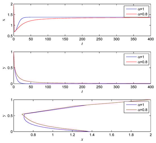
Figure 1.
The stability with , , , , , , , , , .
If one lets , , , , , and , and remain unchanged, then according to Theorem 5, when , , converges to . The simulations are shown in Figure 2.
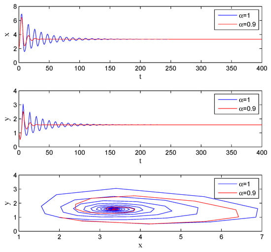
Figure 2.
Stability with , , , , , , , , , .
If one lets , , , , , , , , , , System (5) has an equilibrium point . From Theorem 7, we know that there exists , and the system (5) undergoes Hopf bifurcation at . It can be seen from Figure 3 that with the increase in , the system gradually evolves from stable to unstable.
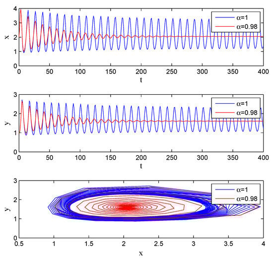
Figure 3.
Stability with , , , , , , , , , .
If one lets , , , , , , , , , , System (5) has an equilibrium point . From Theorem 7, we know that there exists , and the system (5) undergoes Hopf bifurcation at . It can be seen from Figure 4 that with the increase in , the system gradually evolves from stable to unstable.
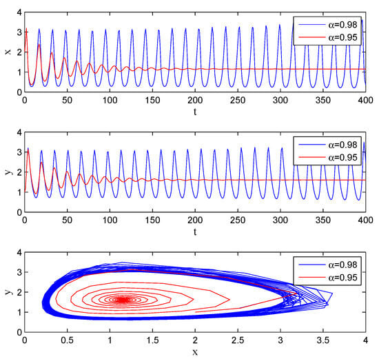
Figure 4.
Stability with , , , , , , , , , .
If one selects , , , , , , , , , , then in Figure 5, we can observe bifurcation of the system with respect to b. In Figure 6, we can observe bifurcation of the system with respect to .
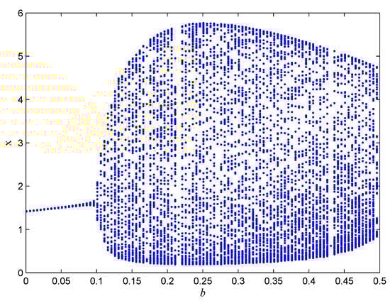
Figure 5.
The bifurcation diagram of the system (5) about b.
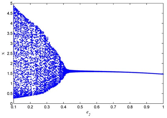
Figure 6.
The bifurcation diagram of the system (5) about .
5. Conclusions
In this paper, a prey–predator model with fear effects in toxic substances is proposed, and the dynamic behaviors of the model, such as uniqueness, boundedness, local stability, global stability, and Hopf bifurcation, are analyzed. It can be verified through theoretical analysis and simulation that the system has a Hopf bifurcation for the fractional derivative and has an influence on the convergence speed and stability of the system. The system also produces bifurcations for parameters b and . It can be seen from Figure 5 and Figure 6 that with the increase in parameter b, System (5) gradually evolves from a stable state to an unstable state; with the increase in parameter , System (5) gradually transitions from an unstable state to a stable state. In the future, we can consider the impact of metabolic issues caused by environmental pollution on the prey–predator model, and whether the fear effect will have a positive impact on the prey.
Author Contributions
Conceptualization, C.L. and Z.W.; methodology, C.L. and Y.C.; software, C.L. and Z.W.; validation, C.L.; investigation, C.L. and Y.Y.; writing—original draft preparation, C.L. and Y.C.; writing—review and editing, Y.Y. and Z.W.; supervision, Z.W.; Funding acquisition, Z.W.; C.L. and Y.C. are the co-first authors. All authors have read and agreed to the published version of the manuscript.
Funding
This work was supported by the Shandong University of Science and Technology Research Fund (2018 TDJH101).
Informed Consent Statement
Not applicable.
Data Availability Statement
Data sharing is not applicable to this article as no datasets were generated or analyzed during the current study.
Conflicts of Interest
The authors declare no conflict of interest.
References
- Wang, Z.; Xie, Y.; Lu, J.; Li, Y. Stability and bifurcation of a delayed generalized fractional-order prey-predator model with interspecific competition. Appl. Math. Comput. 2019, 347, 360–369. [Google Scholar] [CrossRef]
- Lotka, A. Elements of Physical Biology; Williams and Wilkins: Baltimore, MD, USA, 1925. [Google Scholar]
- Liu, M. Dynamics of a stochastic regime-switching predator-prey model with modified leslie-gower holling-type ii schemes and prey harvesting. Nonlinear Dyn. 2019, 1, 417–442. [Google Scholar] [CrossRef]
- Holling, C. The functional response of predator to prey density and its role in mimicry and population regulation. Mem. Entomol. Soc. Can. 1959, 91, 385–398. [Google Scholar] [CrossRef]
- Banerjee, R.; Das, P.; Mukherjee, D. Global dynamics of a Holling Type-III two prey one predator discrete model with optimal harvest strategy. Nonlinear Dyn. 2020, 99, 3285–3300. [Google Scholar] [CrossRef]
- Stanislavsky, A. Memory effects and macroscopic manifestation of randomness. Phys. Rev. E 2000, 61, 4752–4760. [Google Scholar] [CrossRef] [PubMed]
- Kadem, A.; Baleanu, D. Fractional radiative transfer equation within Chebyshev spectral approach. Comput. Math. Appl. 2010, 59, 1865–1873. [Google Scholar] [CrossRef]
- Kaslik, E.; Sivasundaram, S. Dynamics of fractional-order neural networks. IEEE Int. Jt. Conf. Neural Netw. 2011, 59, 611–618. [Google Scholar]
- Mishra, M.N.; Aljohani, A.F. Mathematical modelling of growth of tumour cells with chemotherapeutic cells by using Yang-Abdel-Cattani fractional derivative operator. J. Taibah. Univ. Sci. 2022, 16, 1133–1141. [Google Scholar] [CrossRef]
- Albalawi, K.S.; Mishra, M.N.; Goswami, P. Analysis of the multi-dimensional Navier-Stokes equation by Caputo fractional operator. Fractal Fract. 2022, 6, 743. [Google Scholar] [CrossRef]
- Li, H.L.; Zhang, L.; Hu, C.; Jiang, Y.L.; Teng, Z. Dynamical analysis of a fractional-order predator-prey model incorporating a prey refuge. J. Appl. Math. Comput. 2017, 54, 435–449. [Google Scholar] [CrossRef]
- Creel, S.; Christianson, D. Relationships between direct predation and risk effects. Trends Ecol. Evol. 2008, 23, 194–201. [Google Scholar] [CrossRef] [PubMed]
- Mateo, J.M. Ecological and hormonal correlates of antipredator behavior in adult belding’s ground squirrels (spermophilus beldingi). Behav. Ecol. Sociobiol. 2007, 62, 37–49. [Google Scholar] [CrossRef] [PubMed]
- Peacor, S.D.; Peckarsky, B.L.; Trussell, G.C.; Vonesh, J.R. Costs of predator-induced phenotypic plasticity: A graphical model for predicting the contribution of nonconsumptive and consumptive effects of predators on prey. Oecologia 2013, 171, 1–10. [Google Scholar] [CrossRef] [PubMed]
- Pettorelli, N.; Coulson, T.; Gaillard, D. Predation, individual variability and vertebrate population dynamics. Oecologia 2011, 167, 305–314. [Google Scholar] [CrossRef] [PubMed]
- Zanette, L.Y.; White, A.F.; Allen, M.C.; Clinchy, M. Perceived predation risk reduces the number of offspring songbirds produce per year. Science 2011, 334, 1398–1401. [Google Scholar] [CrossRef]
- Evans, J.P.; Gasparini, C.; Pilastro, A. Female guppies shorten brood retention in response to predator cues. Behav. Ecol. Sociobiol. 2007, 61, 719–727. [Google Scholar] [CrossRef]
- Wang, X.; Zanette, L.; Zou, X. Modelling the fear effect in predator-prey interactions. J. Math. Biol. 2016, 73, 1179–1204. [Google Scholar] [CrossRef]
- Barman, D.; Roy, J.; Alam, S. Trade-off between fear level induced by predator and infection rate among prey species. J. Appl. Math. Comput. 2020, 64, 635–663. [Google Scholar] [CrossRef]
- Das, M.; Samanta, G. A prey-predator fractional order model with fear effect and group defense. Int. J. Dyn. Control 2020, 9, 334–349. [Google Scholar] [CrossRef]
- Barman, D.; Roy, J.; Alrabaiah, H.; Panja, P.; Mondal, S.P.; Alam, S. Impact of predator incited fear and prey refuge in a fractional order prey predator model. Chaos 2021, 142, 110420. [Google Scholar] [CrossRef]
- Pal, S.; Pal, N.; Samanta, S.; Chattopadhyay, J. Effect of hunting cooperation and fear in a predator-prey model. Ecol. Complex. 2019, 39, 100770. [Google Scholar] [CrossRef]
- Sasmal, S. Population dynamics with multiple Allee effects induced by fear factors-A mathematical study on prey-predator interactions. Appl. Math. Model. 2018, 64, 1–14. [Google Scholar] [CrossRef]
- Jensen, A.L.; Marshall, J.S. Application of a surplus production model to assess environmental impacts on exploited populations of Daphnia pulex in the laboratory. Environ. Pollut. 1982, 28, 273–280. [Google Scholar] [CrossRef]
- Nelson, S.A. The problem of oil pollution of the Sea. Adv. Mar. Biol. 1971, 8, 215–306. [Google Scholar]
- Hallam, T.; Deluna, J. Effects of toxicants on populations: A qualitative Approach III. Environmental and food chain pathways. J. Theor. Biol. 1984, 109, 411–429. [Google Scholar] [CrossRef]
- Kar, T.; Chaudhuri, K. On non-selective harvesting of two competing fish species in the presence of toxicity. Ecol. Model. 2003, 161, 125–137. [Google Scholar] [CrossRef]
- He, J.; Ke, W. The survival analysis for a single-species population model in a polluted environment. Appl. Math. Model. 2007, 31, 2227–2238. [Google Scholar] [CrossRef]
- Das, A.; Samanta, G. Modelling the fear effect in a two-species predator-prey system under the influence of toxic substances. Rend. Circ. Mat. Palerm. 2020, 70, 1–26. [Google Scholar] [CrossRef]
- Podlubny, I. Fractional Differential Equations; Academic Press: New York, NY, USA, 1999. [Google Scholar]
- Ye, H.; Gao, J.; Ding, Y. A generalized Gronwall inequality and its application to a fractional differential equation-ScienceDirect. J. Math. Anal. Appl. 2007, 328, 1075–1081. [Google Scholar] [CrossRef]
- Denis, M. Stability results for fractional differential equations with applications to control processing. Comput. Eng. Syst. Appl. 1996, 2, 963–968. [Google Scholar]
- Li, Y.; Chen, Y.; Podlubny, I. Stability of fractional-order nonlinear dynamic systems: Lyapunov direct method and generalized Mittag-Leffler stability. Comput. Math. Appl. 2010, 59, 1810–1821. [Google Scholar] [CrossRef]
- Kai, D.; Ford, N.; Freed, A. A predictor-corrector approach for the numerical solution of fractional differential equations. Nonlinear Dyn. 2002, 29, 3–22. [Google Scholar]
- Kai, D.; Ford, N.; Freed, A. Detailed error analysis for a fractional Adams method. Numer. Algorithms 2004, 36, 31–52. [Google Scholar]
Disclaimer/Publisher’s Note: The statements, opinions and data contained in all publications are solely those of the individual author(s) and contributor(s) and not of MDPI and/or the editor(s). MDPI and/or the editor(s) disclaim responsibility for any injury to people or property resulting from any ideas, methods, instructions or products referred to in the content. |
© 2023 by the authors. Licensee MDPI, Basel, Switzerland. This article is an open access article distributed under the terms and conditions of the Creative Commons Attribution (CC BY) license (https://creativecommons.org/licenses/by/4.0/).