Data Assimilation for Agent-Based Models

Abstract

This article presents a comprehensive review of the existing literature on the topic of data assimilation for agent-based models, with a specific emphasis on pedestrians and passengers within the context of transportation systems. This work highlights a plethora of advanced techniques that may have not been previously employed for online pedestrian simulation, and may therefore offer significant value to readers in this domain. Notably, these methods often necessitate a sophisticated understanding of mathematical principles such as linear algebra, probability theory, singular value decomposition, optimization, machine learning, and compressed sensing. Despite this complexity, this article strives to provide a nuanced explanation of these mathematical underpinnings. It is important to acknowledge that the subject matter under study is still in its nascent stages, and as such, it is highly probable that new techniques will emerge in the coming years. One potential avenue for future exploration involves the integration of machine learning with Agent-based Data Assimilation (ABDA, i.e., data assimilation methods used for agent-based models) methods.

1. Introduction

As data become more widely available at high frequencies, the demand for connecting offline simulation with live data is on the rise. However, there are various challenges associated with linking an offline simulation engine to live data to create a real-time simulation. Real-time simulation refers to a simulation that can be executed at the same rate as a wall clock. These challenges can be broadly categorized into two groups: data-related challenges and simulation engine-related challenges. Data-related challenges include sparsity of data in time and space, the need for real-time data preparation and processing, indirect data (e.g., qualitative data that must be translated into quantitative data), and privacy issues. In addition to the simulation engine’s accuracy and modeling capability, its computational efficiency is also a key concern. This is because some methods require multiple runs of the simulation in real-time, making it essential for the engine to be computationally effective [1].

Furthermore, considering the time required for data preparation, the simulation engine needs to operate much faster than in real-time. This is a significant challenge for agent-based simulations since they usually have high computational costs. The latter has partially led to less attention being paid to real-time (or online ) agent-based simulations [2]. However, due to the increase in computational power and data availability, the research in this field is gaining momentum [1,3,4]. After upgrading the offline simulation to an online one, key applications would be predicting desired attributes, online policy feedback, and resource allocation. Ref. [5] describes how live simulations provide unprecedented applications for disaster response, epidemiology, and computational social science. The authors address various requirements for live simulations ranging from data collection to methodological aspects.

There are various models for simulating pedestrians, and the reader is directed to [6,7,8,9,10] for more information on each type. These models are divided into three main categories: microscopic, mesoscopic, and macroscopic. Among them, microscopic models have gained more attention. These models are programmed at different levels. Ref. [7] specifies them as (a) global path-planning at the highest level, (b) path-following (determining preferred velocity), and (c) local navigation, such as collision avoidance and group behaviour at the lowest level. The local navigation level has been extensively examined in the literature. According to [7], local navigation models that focus on collision avoidance can be categorized into four major types, which can be ordered chronologically as force-based, velocity-based, vision-based, and data-driven-based. Agent-based models are sometimes defined similarly to microscopic models, which is a general point of view. In a more detailed classification, agent-based models are a type of microscopic model in that the agent characteristics (e.g., age and desired velocity) are heterogeneous.

ABMs have been increasingly used in disciplines such as the social sciences, transportation, and economics to simulate large-scale dynamic complex systems. These models are suitable for addressing the emerging behaviours of complex systems. They are flexible and provide a natural description of the system. In these types of models, the behaviour of agents is usually evolved by some rules in a bottom-up approach [11,12]. Therefore, they are a good choice for pedestrian modelling.

Data assimilation (DA), which is a framework created for integrating a model with real-time data to make use of “all available information” [13], exactly addresses the challenges for online agent-based simulation. DA has been extensively used during past decades in Earth sciences (e.g., meteorology) and is incorporated in dynamic data-driven simulation (DDDS) [14,15]. Recently, there have been efforts to replicate the approach for agent-based simulations (e.g., pedestrian simulation) [2,16,17,18,19,20], however, far fewer attempts have been made to move the existing methodology for application in a real-world scenario [1]. Hereafter, we call data assimilation methods used for agent-based models, agent-based data assimilation (ABDA) methods.

In its general meaning, DA will shape the structure of this study by discussing relevant fields to ABDA and examining how other areas can both benefit from and contribute to ABDA techniques. As a result, the reader will understand how literature in (i) detecting and tracking with filtering techniques, (ii) occupancy estimation, (iii) data-driven dynamic systems, and (iv) discrete choice modeling can benefit from each other. This multidisciplinary literature review will widen the readers’ perspective about the underlying pillars of these research areas and hopefully will lead to advancements in all aforementioned fields. Data assimilation, which is a general framework to connect models with data, serves as the stem to connect these leaves. We will start with traditional crowd monitoring systems, which are purely data-based (not incorporating models), and compare them with DA methods so that the reader will better understand the challenges that data assimilation will address. Many of the current real-time pedestrian/passenger monitoring systems do not use simulation engines for crowd monitoring and prediction and are purely data-based [21,22,23].

In a nutshell, the logic behind the review is to first discuss the traditional methods for pedestrian monitoring and then move to the more recent framework, which is data assimilation. Moreover, since pedestrian modelling mainly falls into the agent-based framework, we aim to put focus on data assimilation for agent-based models. Finally, to showcase the potential advantage of the well-established related literature to the relatively new domain of ABDA, we will discuss the literature for that and demonstrate the importance of intersectionality. This article is structured as follows: Section 2 explains the focus of this review, which is a real-time agent-based simulation, and provides statistical information regarding the current publications in this domain. Section 3 elaborates on traditional crowd monitoring systems, their application areas, data collection methods, assesses their shortcomings, and offers the simulation method as an alternative, cutting-edge method, i.e., data assimilation, which can give more broad and detailed information about microscopic pedestrian dynamics. Section 4 reviews the existing data assimilation works, mainly those that incorporate agent-based models. Moreover, the mathematical backgrounds are provided in an integrated way. Section 5 provides a concise overview of research domains that are intimately linked to real-time agent-based modeling and simulation. Section 6 provides an illustration of the intersections between machine learning and data analysis. Section 7 summarizes the primary insights from the literature review. Lastly, the conclusions are presented in Section 8.

2. Method, Scope, and Inclusion Criteria

This current review focuses mainly on real-time agent-based simulation. In this regard, articles have been reviewed in many other fields, such as epidemiology, motorized traffic, robotic navigation, crowd monitoring systems, pedestrian path, and flow prediction. However, our primary aim in referencing them is to analyze contemporary trends in real-time pedestrian monitoring and explore possible intersections. We refer specifically to articles written in the field of crowd monitoring systems (CMS) because the methods for data collection and feature extraction (e.g., flow, density, and velocity) in these articles will eventually be needed to use data assimilation in a real-world scenario. However, most current articles in the field of ABDA have focused more on developing filtering algorithms and using ‘synthetic data’ to test their methods. In addition, the reader can evaluate, based on the application required, whether paying the price to implement real-time simulation is appropriate for them or whether using a traditional CMS technique will get them up and running.

The keywords used in our search process varied for each method. Herein, a quite broad range of keywords and their combinations were used to retrieve information from the SCOPUS database, in addition to the common searches in Google Scholar. The major keywords are summarized in

Table 1. Categorized summary of keywords used in SCOPUS and Google Scholar searches to identify relevant literature in the field of agent-based data assimilation.

Category	Keywords
Method
	reinforcement learning, Kalman filter, particle filter extended Kalman, game, neural network
Technique	data assimilation, data association, modeling, agent-based, multi-agent
Concept
	data-driven dynamic, real-time pedestrian simulation dynamic data-driven
Application	tracking pedestrian, route choice modeling, behavior prediction

. These keywords are systematically organized under distinct heads, encapsulating the multifaceted aspects of ABDA. The “Method" category includes terms such as “reinforcement learning”, “Kalman filter”, “particle filter”, “extended Kalman”, “game”, and “neural network”, indicative of the diverse methodologies employed in ABDA research. The “Technique” category encapsulates keywords such as “data assimilation”, “data association”, “modeling”, “agent-based”, and “multi-agent”, showcasing the varied techniques pivotal for executing ABDA. Under “Concept”, terms such as “data-driven dynamic”, “real-time pedestrian simulation”, and “dynamic data-driven” are included, reflecting the fundamental conceptual frameworks underpinning ABDA. Lastly, the “Application” category incorporates applications in “tracking pedestrian”, “route choice modeling”, and “behavior prediction”, exemplifying the practical implementations of ABDA in real-world scenarios. Moreover, the retrieved query results for the “data assimilation”, “agent-based”, and “agent based” keywords from the SCOPUS database are depicted in Figure 1, which clearly highlights the focus of research in this domain.

3. Traditional Crowd Monitoring Systems

Most traditional methods for online pedestrian monitoring and behavior prediction do not take advantage of any simulation engine [23], and directly work on data and are often coined with the term “Crowd Monitoring Systems (CMS)” in the literature [21]. CMS usually focuses on real-time data collection, feature extraction, and pedestrian tracking. They have been successfully applied in big events management where historical data are usually unavailable. Camera systems [24,25,26,27,28], automatic counting systems [21], RFID sensors [29], Wi-Fi/Bluetooth sensors [21,29,30,31,32,33,34,35,36], GPS sensors [37], social media [38], and transaction cards (e.g., opal in NSW)  [39,40,41,42] are among the data collection methods. Sensor fusion methods can provide more insight into pedestrian behaviour [21,25]. Meanwhile, although camera systems were more prevalent in the past, Wi-Fi/Bluetooth sensors have become the preferred method for data collection. They are cheap, easy to implement, have limited privacy issues, provide good-quality data, and work indoors and outdoors. Moreover, the number of people using smartphones is increasing (larger penetration rate). Pedestrian density, velocity, flow, and path are among the features and parameters that are extracted from data [23].

These features can be used for the prediction of pedestrian variables. For example, refs. [22,39,43,44,45,46,47,48,49] have predicted flow using artificial intelligence and machine learning algorithms. In [50,51], the authors have predicted the pedestrian path using bayesian inference. Although CMSs provide useful tools for real-time crowd management, they do not leverage the power of a sophisticated simulation engine along with real-time data to produce enhanced and comprehensive results. Using a simulation engine can give more broad and detailed information about the microscopic pedestrian dynamics if appropriately combined with online data. This is known as data assimilation, which is currently one of the cutting-edge lines of research in pedestrian/passenger simulation and modeling and will be discussed later in Section 4. It is up to the user, based on the required monitoring task, the availability of data and its quality, and the availability of computational resources, to decide whether to choose traditional CMSs or newborn advanced ABDA methods.

The DA and CMS approaches are cross-compared in

Table 2. CMS vs. DA.

	DA	CMS
Computaional cost	>CMS	DA>
Systemic data noise consideration	🗸	×
Detailed pedestrian dynamic	🗸	×
Handling spatiotemporal sparsity in data	🗸	×
Application in practice	Not Common	Common method

. Potentially, DA methods are a better choice if the computational resource is not a concern. An important reason agent-based data assimilation methods have rarely been used in practice is that this field of research is extremely young. In reality, the necessary steps to implement these methods are still incomplete and being completed. DA methods consider the noise in data and are thus more convenient for real-world scenarios. Moreover, DA methods are well-equipped to tackle spatiotemporal data sparsity systematically, which is something missing in CMSs.

4. Data Assimilation: Integrating Real-Time Data with Simulation Engine

4.1. Dynamic Data Driven Simulation: Data Assimilation Method

The Dynamic Data-Driven Application Simulation (DDDAS) paradigm was first introduced by [52] as a framework to incorporate additional data into an executing application. These data can be archival or collected online and in reverse, have the ability of applications to dynamically steer the measurement process. DDDS is a branch of DDDAS focused on integrating real-time data into simulations. A common method used in DDDS is DA. In general, DA is a framework to utilize both a model and data to take advantage of both to predict the current and future state of the system.

DA is well known for addressing data sparsity in time and space. By using a computer model, data assimilation aims to infer the system state based on incomplete, ambiguous, and uncertain sensor data. A standard data assimilation framework consists of a computer model, a series of sensors, and a “melding” scheme [53]. The Kalman filter, particle filter, and their variants (sequential methods), as well as variational methods such as 3D-Var, and 4D-Var, are among the melding schemes for data assimilation [54]. DA has been widely used for weather prediction, oil and gas pipeline, and ocean and climate modeling [14]. However, more attention should be paid to data assimilation techniques for agent-based models (ABMs) such as pedestrian models. While recent efforts for ABMs are promising, more work should be done to implement them in a complex real-world scenario [2,16,17,18,19,20,55].

4.2. DA for Agent-Based Pedestrian/Passenger Simulations

Due to various reasons, there has been less attention paid toward using DA in agent-based models. First of all, low data availability for agent-based models seems to be the most important. Even for the initialization and offline calibration of agent-based models, adequate data have rarely been available, let alone for use in data assimilation [56]. However, due to advances in real-time data collection methods (Section 3), a more suitable platform has been provided for the implementation of DA methods. Second, the high dimensionality of the state space and the resultant computational cost of ABMs. For this second challenge, due to advances in computational power and the ability to execute DA algorithms in multiple computational nodes, implementing DA methods will be more facilitated in the near future. Just assume that quantum computers are available for use (which is not too far off the mark), then there will be a revolution in implementing these methods. Furthermore, integrating DA with machine learning methods may result in a more efficient performance (Section 5).

EnKF [3,17,20] and particle PF [4,18,57] are the most used methods for ABDA, partly because both methods do not require an analytical form of the state transition model, which is something typical in ABMs. ABMs usually move the system state forward in a black-box fashion, and the analytical formulation may not be feasible due to the ruled-based components of the model. Therefore, methods such as the classical Kalman filter, which requires the analytical form of the transition matrix, could only be used if they are modified for use in ABMs. In Section 1, we will discuss the Bayes filter as a general framework where various ABDA approaches are branched to envision a mathematical big-picture. Almost all ABDA methods fall into the class of sequential data assimilation; therefore, they are based on the prediction (forecast)-correction (update) cycle. VarDA such as three-dimensional variation (3D-VAR) and four-dimensional variation (4D-VAR) have been rarely used with agent-based models, perhaps due to their mathematical complexity. Customizing VarDA methods for ABDA can be a potential direction for future research. In Section 4.4–Section 4.5.2, we will discuss particle filter and Kalman filter-based approaches with their applications in ABDA.

4.3. Bayes Filters

Derived from Bayes’ theorem, the equation is given by:

$$P\left(s_k\right|y_k)\propto P\left(y_k\right|s_k)P\left(s_k\right),$$

(1)

where $s_k$ represents the system state at the $k^{th}$ timestep, and $y_k$ signifies the observation received at the same timestep. The term $P\left(y_k\right|s_k)$ represents the measurement likelihood (which is not necessarily a probability density function), while $P\left(s_k\right)$ denotes the probability distribution of the state obtained by projecting the agent-based model over time. The product of these two terms results in the posterior probability distribution $P\left(s_k\right|y_k)$, which is the primary aim of data assimilation.

In the context of Kalman filters, both terms are assumed to follow a Gaussian distribution. With the Markov assumptions and the linearity of the transition matrix in place, closed-form matrix expressions can be deduced for both the prediction and update phases. The linearity assumption can be relaxed using variants such as the extended Kalman filter, unscented Kalman filter, or ensemble Kalman filter, as discussed in Section 4.5.2. Particle filters, in contrast, make no assumptions about the distribution’s probability and linearity. This robust, “brute-force” method is apt for agent-based models that employ nonlinear transition matrices and non-Gaussian (categorical) state variables. Such categorical parameters, such as an agent’s destination, are frequently observed in ABMs and present challenges for the standard Kalman filter and its variants [2]. One significant limitation of particle filters for real-time applications is the large number of particles needed, leading to substantial computational costs. Ensemble Kalman filters are another popular approach in agent-based data assimilation. Unlike particle filters, ensemble Kalman filters draw ensembles from a normal distribution.

The particle filter, the unscented Kalman filter (UKF), and the ensemble Kalman filter are explored further in Section 4.4, Section 4.5.1 and Section 4.5.2, respectively, representing the major methodologies in current literature. Notably, [58] introduced a pioneering method for agent-based data assimilation by applying quantum mechanics field theory to reinterpret Equation  (1) using annihilation and creation operators. The integration of reinforcement learning and other machine learning strategies can also be fruitful, as indicated by [59,60]. However, as of our latest understanding, no machine learning method has been firmly established with consistent outcomes for ABDA.

4.4. Particle Filter

Particle filtering has been extensively employed in geophysical systems. Each particle represents an instance of the model. Denoting the number of particles as $N_p$, the particle set as $M_k$, the state of the $i^{th}$ particle at timestep $t=k$ as $x_k^i$, and its weight as $w_k^i$ such that ${\sum }_{i=1}^N{w}_k^i=1$, we can express the particle set as:

$$M_k=\{<x_k^i,w_k^i>\mid i=1,...,N\}$$

(2)

Particles aim to estimate the posterior distribution of the system state, $x_k$, based on a Monte Carlo method combined with a first-order Markov process. These particles are essentially samples from the probability distribution. They are advanced in time by the transition model, and their weights are updated when a new system observation becomes available. These weights are influenced by the proximity of the particles to the received observations (sensor data). Higher weight is given to particles, which more accurately estimate the true state variables. Subsequent to weight adjustment, particles are resampled, leading to the modification or deletion of low-performing particles  [1]. To avert particle collapse, random noise (such as Gaussian white noise) is typically introduced. Particle collapse refers to situations where only a handful of particles have substantial weights, rendering most of the particles ineffective and lacking in diversity.

Various particle filter algorithms have been proposed and applied to different tasks. The basic particle filter with importance sampling neither resamples particles nor modifies them; it solely updates the particle weights. Such an approach is beneficial when there is substantial prior knowledge about the true state residing within the set of particles [61]. Sequential Importance Resampling (SIR) is an extension of the basic importance sampling algorithm and is commonly used for agent-based data assimilation. However, challenges such as divergence can arise even with resampling [1]. Addressing these issues, researchers have proposed enhancements and new methods. For instance, Ref. [4] introduced a particle filter with a mixed component set resampling to tackle particle deprivation. Ref. [57], inspired by both [4,62], employed SIR PF and introduced “jittering” (adding white Gaussian noise to particles) to counteract particle deprivation [63]. Ref. [1] modified the resampling method to retain certain inferred parameters of low-weight particles. A noteworthy integration is presented by [64], who combined the PF algorithm with a behavior pattern detection model, which was executed by a Hidden Markov Model (HMM). This model recognizes behavior patterns at each data assimilation step, allowing for a more nuanced sampling.

Several parameters play a pivotal role in the construction of the particle filter algorithm, such as the number of particles $N_p$, data assimilation frequency (or DA “window”), and the distribution of particle noise. The number of particles, in particular, is crucial for performance and computational efficiency. Ref. [65] proposed a threshold, as follows:

$$\begin{array}{c}\hfill N\gg exp\left(\frac{{\tau }^2}{2}\right)\end{array}$$

(3)

with a comprehensive proof available in their paper. As an approximation, ${\tau }^2$ can be viewed as the number of independent observations, a metric backed by numerous studies [61]. This formula indicates that as state dimensionality grows, particle requirements increase exponentially. Moreover, particle filters have seen applications in traffic estimation [66] and epidemiology [67,68], among others. In epidemiology, [69] initiated the application of particle filters, while [70] introduced the Smart Beam Particle Filter (SBPF) for epidemic forecasting.

4.5. Kalman Filter

The Kalman filter, rooted in state–space analysis, is a linear, discrete, and recursive estimation approach. It extends the Weiner filter to handle non-stationary scenarios [71]. This filter relies solely on the previous step’s information to recursively estimate the state in a noisy linear dynamical system, aiming to minimize the mean squared error. For a discrete-time dynamical system [72], the model can be defined by:

$$\begin{array}{cc}\hfill x_k& =F_k{x}_{k-1}+G_k{u}_k+w_k\hfill \end{array}$$

(4)

$$\begin{array}{cc}\hfill y_k& =H_k{x}_k+v_k,\hfill \end{array}$$

(5)

where $x_k\in {\mathbb{R}}^n$ is the state, $y_k\in {\mathbb{R}}^q$ the measurements, and $u_k\in {\mathbb{R}}^p$ represents a known sequence of inputs. $w_k$ and $v_k$ denote uncorrelated zero-mean random noise processes. The matrices $Q_k$ and $R_k$ serve as positive–definite covariance matrices for process and sensor noise, respectively. The transition function F originates from the discrete representation of the physical model, and H is the observation function relating the true state to the observations. The system’s initial state is defined as $x_0={\mu }_0+w_0$, where ${\mu }_0\in {\mathbb{R}}^n$ is known.

Upon minimizing pertinent cost functions, we derive the following formulas for the forecast and update steps:

$$\begin{array}{cc}\hfill P_{k|k-1}& =F_k{P}_{k-1}{F}_k^T+Q_k\hfill \end{array}$$

(6)

$$\begin{array}{cc}\hfill {\widehat{x}}_{k|k-1}& =F_k{\widehat{x}}_{k-1}+G_k{u}_k\hfill \end{array}$$

(7)

$$\begin{array}{cc}\hfill K_k& =P_{k|k-1}{H}_k^T{(H_k{P}_{k|k-1}{H}_k^T+R_k)}^{-1}\hfill \end{array}$$

(8)

$$\begin{array}{cc}\hfill {\widehat{x}}_k& ={\widehat{x}}_{k|k-1}+K_k(y_k-H_k{\widehat{x}}_{k|k-1}),\hfill \end{array}$$

(9)

$$\begin{array}{cc}\hfill P_k& =(I-K_k{H}_k)P_{k|k-1}\hfill \end{array}$$

(10)

For nonlinear systems characterized by:

$$\begin{array}{cc}\hfill x_k& =f_k(x_{k-1},u_k)+w_k\hfill \end{array}$$

(11)

$$\begin{array}{cc}\hfill y_k& =h_k\left(x_k\right)+v_k,\hfill \end{array}$$

(12)

extensions of the classical Kalman filter, such as the unscented and ensemble Kalman filters, are utilized in ABDA [2]. The unscented Kalman filter (UKF) bridges the gap between the low computational cost of the ensemble Kalman filter and the high performance of the particle filter.

4.5.1. Unscented Kalman Filter (UKF)

Introduced by [73], the UKF utilizes weighted sigma points (ensembles) propagated to the next timestep by the non-linear transition function. A Gaussian distribution is then optimally fitted to these sigma points. The steps of this algorithm can be outlined as [2,74]:

1. Prediction: From the state distribution at $t=k-1$, sigma points (${\chi }_{k-1}^{\left[i\right]},i=0,\dots ,2n$) and their weights ($w_{k-1}^{\left[i\right]}$) are deterministically computed. For the detailed mathematical formula concerning the selection of sigma points and their weights, refer to [73,74].

2. Update: Similar to the classical Kalman filter, the update step assimilates observations with the model prediction.

Moreover, several advancements and applications of the UKF in the context of agent-based data assimilation are discussed in [2,75].

4.5.2. Ensemble Kalman Filter

The ensemble Kalman filter (EnKF) was pioneered by [76]. Compared to the computational complexity of the extended Kalman filter or the unscented Kalman filter, EnKF offers simplicity. The primary computational challenge might arise from matrix inversion, particularly when addressing large datasets [77,78]. Despite its widespread use in pedestrian trajectory prediction, there is still potential for its application in ABDA [50]. EnKF and PF both employ the Monte Carlo method and address the non-linearity of the ABMs. EnKF, however, is more computationally efficient than PF due to the smaller number of ensembles required for real-time simulation. Given its intuitive implementation, it often serves as the starting point for many researchers [56]. This simplicity stems from the Monte Carlo sampling approach for pdf estimation, which allows the classic Kalman filter formulas (as illustrated in Equations (8) and (9)) for linear systems to be extended to non-linear ones by substituting the covariance matrix with the sample covariance. One limitation is its inherent Gaussian approximation [79].

The EnKF methodology consists of two primary stages: prediction and update, as follows:

1. Prediction: during this phase, the state of the system evolves with assistance from the simulation engine. Contrasted with the forecast step of the classic Kalman filter (illustrated in Equations (6) and (7)), where there is no analytical formulation for the state transition matrix F, the ensemble mean approximates the system’s true state. The associated covariance denotes uncertainty [56]:

$$\begin{array}{c}\hfill {\widehat{x}}_k=\frac{1}{N}\sum _{i=1}^N{x}_k\left(i\right)\end{array}$$

(13)

$$\begin{array}{c}\hfill P_k=\frac{1}{N-1}\sum _{i=1}^N(x_k\left(i\right)-{\widehat{x}}_k){\left[(x_k\left(i\right)-{\widehat{x}}_k)\right]}^T,\end{array}$$

(14)

here, N represents the number of ensembles, $x_k\left(i\right)$ each ensemble forecast, ${\widehat{x}}_k$ the ensemble forecast average, and $P_k$ the ensemble covariance. It is logical for the covariance to decrease when new observations become available, especially in agent-based models with a consistent agent count. The update or DA step incorporates observations with ensemble predictions.

2. Update: for this step, the formulas employ a matrix representation akin to Equations (8) and (9) for each ensemble:

$$\begin{array}{c}\hfill K_k=P_k{H}_k^T{(H_k{P}_k{H}_k^T+R_k)}^{-1}\end{array}$$

(15)

$$\begin{array}{c}\hfill {\widehat{x}}_k^a\left(i\right)={\widehat{x}}_k\left(i\right)+K_k(y_k-H_k{\widehat{x}}_k\left(i\right)),\end{array}$$

(16)

here, ${\widehat{x}}_k^a\left(i\right)$ represents the assimilated state for the $i^{th}$ ensemble, and ${\widehat{x}}_k\left(i\right)$ denotes the predicted state obtained by advancing the simulation engine from the previous timestep ($k-1$). The updated ensemble mean ${\widehat{x}}_k^a$ and covariance $P_k^a$ post-data assimilation are:

$$\begin{array}{c}\hfill {\widehat{x}}_k^a=\frac{1}{N}\sum _{i=1}^N{x}_k^a\left(i\right)\end{array}$$

(17)

$$\begin{array}{c}\hfill P_k^a=\frac{1}{N-1}\sum _{i=1}^N(x_k^a\left(i\right)-{\widehat{x}}_k){\left[(x_k^a\left(i\right)-{\widehat{x}}_k)\right]}^T\end{array}$$

(18)

This procedure continues until the final observation is processed.

In their work, [56] explored EnKF for agent-based data assimilation. However, the foundational model they presented was notably simplistic and might not meet specific criteria for an agent-based model [57]. They assessed the performance of EnKF on two models, namely the “box” and “WHIRS”. For the box-model, EnKF was applied on pseudo-truth data aiming to estimate population counts. In contrast, the WHIRS-model, an agent-based one, was used to estimate a fixed-size state vector, employing real-world data to train the EnKF. To address the limitation of fixed state size, they suggest setting the state size equivalent to the maximum feasible agent count. Ref. [17] employed EnKF in a train station atrium scenario but excluded categorical parameters, indicating ongoing research to adapt EnKF for such parameters. Ref. [80] used real-world data to estimate the parameters of the PEDFLOW [81] model, namely for a unidirectional experiment and the Maataf in Kaaba. They highlighted the need for varying parameter values across scenarios, underscoring the role of data assimilation for ABMs. Finally, Ref. [3] utilized EnKF for both model parameter optimization and state estimation. However, they found the EnKF’s performance wanting in terms of state estimation, attributing this partly to the randomness level of their model. A quick summary is provided in

Table 3. Summary of previous works of data assimilation for pedestrian movement.

Paper	Method	Estimated Variables	Number of Agents	Number of Ensembles (Particles)	Sampling/Resampling Method	Efficacy Metric	Observation Source	Main Finding or Application
[2]	RJUKF	Agents’ location, Destination	10, 20, 30	—	N.A	Grand median L2 norm between estimated and true locations, Indicator function(for destination)	Synthetic data	Combining RJMCMC with UKF
[75]	UKF	Agents’ location	10, 20, 30	—	N.A	Grand median L2 norm between estimated and true locations	Synthetic data	Applying UKF for ABDA for the first time
[4]	PF	Agents’ location, Destination	1–6	800–2000	Standard +mixed component	Average of L2 norm	Synthetic data	New resampling method
[62]	PF	Agents’ location+behavior (both integer)	100	50	Metropolis-Hastings (M-H)	Absolute distance between normalized particle count and true count(summed over all nodes)	Synthetic data	PF for evacuation scenario + mapping method for efficient measurement update
[57]	PF	Agents’ location	2–40	1–10,000	SIR	Median of mean L2 norm between estimated and true Agnets’ locations	Synthetic data	Attempting to apply data assimilation to a system that exhibits emergence—Performing extensive experiments to assess PFs for DA
[57]	PF	Agents’ parameters, variables and global model parameter	2–40	1–10,000	SIR	Median of mean L2 norm between estimated and true Agents’ state	Synthetic data	Performing extensive experiments to assess PFs for DA
[1]	PF	Agents’ location+destination+desired speed	274	5000	SIR+ Adapted SIR	Mean distance	CCTV camera	Adapted resampling method + testing PF on real world scenario (proof of concept)
[18]	PF	Trajectory	323–2299	108–640	Custom	RMSE of destinations	Real world trajectory	Model based method for estimating people flow
[64]	PF	Agents’ location+destination+velocity	—-	—	—	—	—	Behavior pattern informed data assimilation
[17]	EnKF	Agents’ location	20	10	N.A	Distances	Synthetic Data	Applying EnKF to ABM
[3]	EnKF	Agents’ location +model parameters	600	30	N.A	RMSE	Synthetic data	AMB parameter optimization
[56]	EnKF	Num. of people +model parameters	(0, 19,820)	1, 100, 1000	N.A	RMSE	Synthetic data + camera counts	Applying EnKF to ABM
[80]	EnKF	Model parameters	middle to high (more than 1000)	20,32	N.A	costume cost function	Camera	Applying EnKF for ABM calibration
[16]	Genetic algorithm	parameter estimation	10 k–100 k	N.A	N.A	Nash–Sutcliffe model efficiency coefficient (NSE)	Camera count + GPS	78.1% accuracy for $2^{2100}$ parameter space

and 

Table 4. Comparison of different data assimilation methods.

Characteristic	PF	EnKF	RJUKF	UKF
Computational cost	High	Less than PF	Less than EnKF	Less than EnKF
Categorical variables	🗸	×	🗸	×
Non-linearity	🗸	🗸	🗸	🗸
Closed form formula	×	🗸	×	🗸
Assumption on pdf form	×	🗸	🗸	🗸

.

5. Relevant Fields

In this section, a concise overview of research domains that are intimately linked to real-time agent-based modeling and simulation is provided, including:

• Tracking and predicting pedestrian trajectories.
• Occupancy estimation in smart buildings.
• Integration of machine learning and data assimilation, often referred to as “data learning” [82].
• Discrete choice models.

It is worth noting that the methodologies employed in tracking and predicting pedestrian trajectories bear a striking resemblance to the state-of-the-art techniques in ABDA. Enthusiastic readers might find inspiration from studies in this domain for applications in ABDA (Section 5.1). Pioneers in the realm of smart buildings have been instrumental in the advancement of agent-based data assimilation [64] (Section 5.2). In Section 5, several publications have delved into the confluence of machine learning and data assimilation. However, a standardized framework for integrating machine learning into ABDA is still in its infancy. The amalgamation of machine learning and data assimilation in alternative modeling paradigms might offer valuable insights.

5.1. Detecting and Tracking Using Filtering Techniques

The study of detecting, tracking, and predicting pedestrian paths in areas with a network of sensors, predominantly CCTV cameras, predates the real-time simulation of pedestrian movements. A myriad of articles delve into this topic, substantially outnumbering those on real-time pedestrian simulations. Remarkably, several methods applied for pedestrian tracking echo those used in real-time simulations, such as the use of Bayes filters and pedestrian motion models. Consequently, real-time pedestrian simulations utilizing data assimilation can be viewed as expanded versions of tracking methods. Although pedestrian tracking encompasses diverse techniques, those methods that incorporate a pedestrian motion model, especially agent-based models, alongside real-time data for tracking and path prediction are directly relevant. Noteworthy methods in this domain are discussed to provide insight. For a comprehensive survey of other tracking methodologies, the reader is directed to [8,83].

In [84], an algorithm merging a particle filter with the environment’s Voronoi graph is proposed for pedestrian tracking. The study utilizes two distinct types of ID sensors: 73 Versus infrared receivers and 3 Cricket ultrasound receivers, both notorious for producing false-negative readings. Leveraging the Voronoi graph, the authors implement the Expectation-Maximization (EM) algorithm for clustering pedestrian movement patterns. Contrary to trackers that employ rudimentary motion models based on constant velocities or accelerations, Ref. [85] amalgamates the social force model with a Kalman filter-based multi-hypothesis tracker.

The contributions of Bera et al. stand out in this field [28,50,86,87]. Particularly, Ref. [50] is salient for its incorporation of intricate pedestrian motion models in real-time tracking. The researchers exploit both EnKF and EM for real-time pedestrian path prediction, utilizing global and local movement patterns (GLMP). Their comprehensive approach, which does not necessitate prior learning, reportedly outperforms conventional models by 12–18%. The various works discuss the amalgamation of different pedestrian movement models with particle filter trackers, demonstrating advancements in accuracy and computational efficiency.

5.2. Occupancy Estimation

Modeling and analyzing pedestrian behavior serves a plethora of objectives. In transportation contexts, the focal concerns are pedestrian safety, decision-making regarding exit choices, and overarching parameters imperative for pedestrian management. Contrastingly, engineers striving to optimize energy consumption in edifices view pedestrian dynamics from a unique lens, primarily encapsulated by “occupancy estimation”. Such studies predominantly emphasize the interplay between occupants and the infrastructure to foster intelligent energy consumption. Precise occupancy information can, for instance, enable the fine-tuning of heating or cooling systems. In evacuation scenarios, the paradigms of transportation and occupancy estimation converge as evacuative movements in smart buildings and transportation nodes exhibit analogous patterns. As defined by [88], occupancy not only pertains to human presence but also encapsulates actions undertaken to influence the indoor environment.

Ref. [89] is a trailblazing study that leveraged the extended Kalman filter (EKF) for occupancy estimation during egress and a simple Bayes filter for conventional building modes. Their methodology, tested on both agent-based simulations and real-world fire alarms, exemplifies the potential of these techniques. Ref. [90] introduces a real-time occupancy estimation algorithm capitalizing on environmental sensors. These sensors, measuring parameters such as $C{O}_2$, temperature, and humidity, offer the advantage of being non-intrusive and pose minimal privacy concerns. A series of investigations by researchers at Georgia State University delve into occupancy estimation in smart environments via ABDA [4,53,64,91,92], with a detailed exploration provided in Section 4.

5.3. Data-Driven Dynamic Systems

Data-driven dynamic systems aim to understand the underlying dynamics of systems using data. Integrating these with traditional DA methods can enhance the assimilation process. Broadly, these methods fall into two categories:

• Machine learning-based methods, which largely operate within a black-box framework.
• Analytical approaches that strive to derive the governing equations of the dynamical system.

The latter methods have been pioneered by works such as [93], which introduced the Sparse Identification of Nonlinear Dynamics (Sindy) to determine the equations governing a dynamical system. This method leans heavily on the sparsity assumption, previously introduced in compressed sensing [94,95]. It has been effectively applied in areas such as fluid dynamics, even reproducing the Navier–Stokes equations [96,97]. Notably, Sindy offers explicit law-based generalisation, a feature elusive to AI and machine learning techniques. Another notable method in this domain is symbolic regression. Ref. [98], for instance, combined symbolic regression with deep learning to tackle challenges such as high-dimensionality and generalisation. We believe a sparsity-based formulation may assist the model in updating as new data arrive [99]. Machine learning-based methods will be further explored in the following section.

Machine learning (ML) techniques have found applications in data assimilation, especially within the realm of earth sciences. However, its use in ABDA remains relatively uncharted, suggesting promising avenues for future research. Both ML and DA fundamentally rely on optimization, and given ML’s adeptness at approximating nonlinear functions, a collaboration between the two seems intuitive [82]. Applications vary; some researchers replace components of the DA process, such as the likelihood calculation, with ML algorithms [100], while others entirely overhaul the DA procedure [101]. Yet another approach involves substituting the state transition function with an artificial neural network (ANN), referred to as a surrogate function [102]. One of ML’s main contributions to DA is its potential to expedite the assimilation process.

Regarding network architectures, recurrent neural networks (RNNs), such as LSTM and Elman networks [103], along with feed-forward networks such as MLP, are dominant in merging ML with DA. These methods typically employ supervised learning, using targets generated by the assimilation process. ANNs, when applied to DA, essentially approximate functions [104]. Both feed-forward and RNNs have been mathematically validated as effective approximators [105,106].

While RNNs excel at handling sequence-dependent problems owing to their inherent memory, LSTMs shine in recognizing long-term dependencies and addressing the vanishing gradient issue prevalent in standard RNNs. An LSTM unit features three primary gates: update, forget, and output. Ref. [107] noted that the E-NN model outpaces the MLP in terms of speed and offers reduced complexity (fewer neurons). However, the MLP remains superior in accuracy. Being a traditional neural network, MLP can aptly fit any measurable function and is frequently used to emulate the DA process.

Initial attempts to incorporate ML in the DA process are captured in works such as [108,109,110]. For example, Ref. [109] highlighted the parallels between variational data assimilation and neural networks, particularly in their mutual goal of cost function minimization. Subsequent studies [101,102,111,112,113,114,115,116,117,118] further built on these initial insights, each introducing innovative methods and algorithms to further the integration of ML and DA. Interested readers are directed to the comprehensive studies by Arcucci et al. at the data mining lab at Imperial College London. Overall, with the development of efficient and powerful machine learning techniques, along with abundant data availability, the future perspective for DA is expected to be based on autonomous and smart ML models. The machine learning methods for DA are summarized in

Table 5. Machine learning methods for data assimilation.

Paper	NN Type	Integrated DA Method	Dynamical Model
[108]	MLP	KF	Lorenz model
[119]	-	Statistical Interpolation(SI)	Wave model
[111]	MLP	PF	Lorenz model
[120]	MLP	KF	Three-wave model
[121]	MLP	Variational	Lorenz model
[122]	MLP	Variational	Wave model
[107]	Elman	KF	Shallow water 1D model (DYNAMO-1D)
[104]	RBF	KF	Shallow water 1D model (DYNAMO-1D)
[112]	MLP	LETKF	Atmospheric general circulation model (FSUGSM)
[123]	MLP	LETKF	Atmospheric general circulation model (SPEEDY)
[124]	Mixed Type	KF	Satellite-Derived Sea Surface Temperature data
[125]	Fully Connected	Variational, KF	Dot system and Lorenz models
[117]	LSTM	Variational (3DVAR)	CFD model (Fluidity)
[114]	Elman	Variational	Dot system and Lorenz models
[102]	LSTM	KF	CFD model (Fluidity)
[101]	MLP	Variational	Lorenz model
[126]	LSTM	Variational	Lorenz model
[127]	MLP	Variational and EnKF	Lorenz model
[118]	LSTM	KF	Oxygen diffusion across the Blood–Brain Barrier model

.

5.4. Discrete Choice Models

A discrete choice model can be expressed as [128]:

$$y=h(x,ϵ)$$

(19)

where x denotes observed factors, $ϵ$ represents unobserved factors, and y signifies the choice model outcome. Given the observed factors, the probability of y can be articulated as:

$$P(y|x)=\int I[h(x,ϵ)=y]f(ϵ)dϵ,$$

(20)

here, I is an indicator function that assumes a value of 1 when $h(x,ϵ)=y$ and 0 otherwise. Imposing specific assumptions on h and f leads to diverse choice models. For instance, by assuming an i.i.d extreme value distribution for $f\left(ϵ\right)$, and defining $h(x,ϵ)$ as

$$h(x,ϵ)=\sum _{i\in \{1,2,...,J\}}i\times I[U_{ni}>U_{nj}]$$

with y belonging to $\{1,2,...,J\}$, we obtain the closed-form logit choice probability:

$$P_{ni}=\frac{e^{V_{ni}}}{{\sum }_j{e}^{V_{nj}}}$$

(21)

In this context, $B=\{1,2,...,J\}$ denotes the alternative set, while $V_{ni}$ is the sum of observed $U_{ni}$ and unobserved ${ϵ}_{ni}$ components of the utility.

Though the logit model precludes the integration of individual-level parameters, certain discrete choice models, such as the mixed logit, alleviate this constraint. However, integrating these parameters can complicate the estimation process. When viewed through the lens of a data assimilation framework, this approach empowers modelers to estimate individual-level parameters, creating avenues to incorporate other state variables in the estimation process. This becomes particularly valuable when considering time-dependent (or dynamic) networks.

Ref. [129] demonstrates that a logit model could be viewed as an ANN. According to [118], we know that data assimilation has the potential be formulated as ANN, which paves the way to combine data assimilation with discrete choice models. Ref. [130] utilized machine learning techniques for automatic “feature selection”. Using a Bayesian approach and automatic relevance determination (ARD), they devised a data-driven method, DCM-ARD, which can ascertain the optimal utility function [99]. This method assesses potential variables in the function and provides relevant parameters for each. High values indicate probable inclusion in the optimal utility function. This approach builds on machine learning’s regularization-based feature selection, notably the LASSO method and is suitable for the live-stream of data (online learning).

6. Bridging Machine Learning and Data Assimilation: A Case Study on Particle Filters

In order to showcase an example of how the kind of literature discussed in Section 5 can contribute to the ABDA, in this section we shall borrow some concepts from learning guarantees, as proposed by [131]. We aim to illustrate how these concepts can be integrated into the particle filter, starting with the introduction of the PAC framework in Section 6.1, and applying it to the particle filter in Section 6.2.

6.1. Probabilistically Approximate Correct (PAC) Framework

The PAC framework, as defined by [131], states that “a concept class C is PAC-learnable if an algorithm exists, and a polynomial function $poly(, , , )$, such that for any $ϵ>0$ and $\delta >0$, for all distributions D on X and for any target concept $c\in C$, the following holds for any sample size $m⩾poly(1/ϵ,1/\delta ,n,size(c\left)\right)$”:

$$P_{S\sim D^m}[R\left(h_s\right)⩽ϵ]⩾1-\delta ,$$

(22)

where $R\left(h_s\right)$ represents the generalisation error of the hypothesis $h_s$.

Consider the following theorem presented by [131]: Theorem (Learning bound; finite H, consistent case): let H be a finite set of functions mapping from X to Y. Let A be an algorithm that for any target concept $c\in H$ and i.i.d. sample S returns a consistent hypothesis $h_S:\widehat{R}S\left(hS\right)=0$. Then, for any $ϵ,\delta >0,$ the inequality $P_{S\sim D^m}[R\left(h_s\right)⩽ϵ]⩾1-\delta$ holds if:

$$m⩾\frac{1}{ϵ}\left(log\right|H|+log\frac{1}{\delta })$$

(23)

This sample complexity result can be restated as a generalisation bound: for any $ϵ,\delta >0$, with a probability of at least $1-\delta$:

$$R\left(h_s\right)⩽\frac{1}{m}\left(log\right|H|+log\frac{1}{\delta })$$

(24)

6.2. Particle Filter Derivation

Let us denote the hypothesis set by H, which in our case is the particle set M. We have:

$$\begin{array}{c}\hfill m⩾\frac{1}{ϵ}\left(log\right|M|+log\frac{1}{\delta }),\end{array}$$

(25)

where $\left|M\right|$ is the cardinality of the particle set and is finite. We have assumed a particle (simulation instance) in the particle set, $P^{*}$, which results in zero error after some assimilation windows (consistent case). In this setup, each assimilation window is viewed as a training sample and the learning algorithm is seen as the method of likelihood calculation.

The formula above suggests that for a learning task with particles as its hypothesis set, the data quantity required to achieve $1-ϵ$ accuracy, and $1-\delta$ certainty (number of assimilation steps in our case) is at least $\frac{1}{ϵ}\left(log\right|M|+log\frac{1}{\delta })$. Particle collapse can be envisioned as a scenario where a particle is learned over some iterations. Under this assumption, the number of iterations for particle collapse might be correlated to $\frac{1}{ϵ}\left(log\right|M|+log\frac{1}{\delta })$. Hence, we can suggest, with $1-ϵ$ accuracy and $1-\delta$ certainty, that the number of iterations to particle collapse is related to $log\left|M\right|$. In other words, the particle collapse will be delayed at a logarithmic rate with a larger particle set. However, the derivations above are based on strong assumptions, and a genuine particle filter experiment without these simplifications can either verify or contradict this proposition.

6.3. The Concept of Covering Number in Particle Filters

In this section, the concept of a covering number is introduced within the context of particle filters. We consider a particle filter with a particle set M whose cardinality is $\left|M\right|$. This filter is a mapping from X to Y. The covering number for this particle set, denoted as $N(M,ϵ)$, is defined as k. This definition implies that for any given particle within the set, denoted as $M_j$, there exists another particle, $M_i$, within the subset $M_1,M_2,\dots ,M_k$. This latter particle satisfies the condition that ${max}_{x\in X}|M_j\left(x\right)-M_i\left(x\right)|<ϵ$.

The covering number serves as a metric that quantifies the diversity within the particle set. As such, a particle set characterized by a larger covering number is generally more desirable. Given the condition that ${max}_{x\in X}|M_j\left(x\right)-M_i\left(x\right)|<ϵ$ must be upheld for all $x\in X$, it follows logically that finding a pragmatic way to calculate the covering number is imperative. One potential method for doing this involves taking a subset of X to compute the covering number. It is noteworthy that covering numbers has been employed in the field of machine learning to establish mathematical guarantees. These guarantees are aimed at constraining the generalization error. Therefore, covering numbers not only provides a measure of efficiency but may also be instrumental in developing mathematical assurances for particle filters.

6.4. Online Learning and Its Implications for Particle Filtering

The fundamental construct of online learning can be succinctly described as follows: in each round, an algorithm receives an input and formulates a prediction predicated on expert advice. Following this, the actual labels are presented, and a loss function is computed. The paramount objective is the minimization of the regret function. This is articulated as the cumulative loss minus the least loss sustained by the leading expert. In the online learning paradigm, data undergo processing during every round, offering advantages such as computational efficiency, practicality, and straightforward implementation. Two primary attributes differentiate online learning from other learning paradigms:

1. It operates without distributional assumptions, eschewing the generalization concept. Instead, algorithmic performance hinges on the regret notion.

2. The learning and testing phases are interspersed, a deviation from the assumptions in Probably Approximately Correct (PAC) learning.

Drawing parallels between online learning and sequential data assimilation methodologies reveals some intriguing similarities. As an exemplar, consider the classical Exponential Weighted Average (EWA) algorithm (Listing 1):

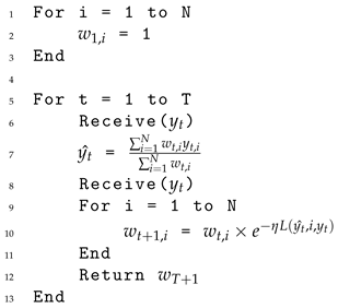
Listing 1. EWA algorithm

The particle filter can be perceived as a variant of the EWA algorithm. By viewing each particle forecast as expert advice, the state vector as input, and aligning the likelihood calculation (alongside its subsequent update rule) with the weight update in line 9 of the aforementioned algorithm, such a parallel becomes evident. As indicated by [132], the weight update formula for the particle filter can be expressed as:

$$w_{j+1}=g_j\left({\widehat{v}}_{j+1}\right)w_j,$$

(26)

where:

$$g_j\left({\widehat{v}}_{j+1}\right)\propto P\left(y_{j+1}\right|v_{j+1})$$

(27)

It is worth noting that mathematical guarantees prevalent in online learning might be conducive for adaptation to the particle filter realm. Taking the theorem from [131] as an illustration, it states that under conditions where the loss function L is convex with regard to its primary argument and assumes values in the range $[0,1]$, the regret of the EWA algorithm after T rounds is:

$$R_T⩽\frac{logN}{\eta }+\frac{\eta T}{8}$$

(28)

Specifically, when $\eta =\sqrt{8logN/T}$, the regret is capped at:

$$R_T⩽\sqrt{\frac{T}{2}·logN}$$

(29)

Leveraging the above guarantee for particle filtering mandates us to redefine the loss accrued by each particle in a manner that aligns with the theorem’s prerequisites. Upon contrasting the weight update rules in both algorithms, we ascertain:

$$g=e^{-\eta L}$$

(30)

Given that $L\in [0,1]$, it is logical to infer:

$$0<\frac{-1}{\eta }ln\left(g\right)<1,$$

(31)

On the assumption that the g function (derived from the likelihood) satisfies:

$$e^{-\eta }<g<1$$

(32)

It can be deduced that the equation holds for the particle filter when the convex loss function is articulated as:

$$L=\frac{-1}{\eta }ln\left(g\right)$$

(33)

Examining the proof approach in [131] and revisiting the Hoeffding inequality [133], one can broaden the loss function’s domain such that:

$$R_T⩽\frac{logN}{\eta }+\frac{\eta T}{8}{(b-a)}^2$$

(34)

Expanding the discourse to include another rendition of the EWA forecaster, we can base our discourse on the work of [134] as it relates to geodesic spaces. A comprehensive exploration of the notations is available in [134]. According to the same source, the primary advantage of the geodesic interpretation of the EWA and its accompanying regret bound for particle filters lies in the flexibility it provides in the utilization of diverse decision spaces, all the while ensuring that regret remains bounded.

7. Results and Discussion

Even though many algorithms used in real-time pedestrian/passenger simulation have been applied for decades in other fields, real-time simulation responding to live data remains a nascent research area that has gained momentum recently. The principal methods used so far for ABDA include particle filter, Kalman filter, and their extensions (Table 4). Most methods have certain limitations for implementation in the real world; for example, they assume that the system’s boundary conditions (input) are known over time. This can be true in places such as train stations where people’s entrance is recorded via station gates, but for other scenarios, appropriate arrangements must be made both for data collection and methodology development in order to determine the input of the system even in a situation where data cannot be obtained as easily as a train station over time and space. Using ML and time series methods can be a good option for this purpose. Only some attempts have been made to integrate ML methods in ABDA [135], and we believe there will be more work on this topic in the near future.

Among the articles reviewed, it is rare to find an article that uses a sophisticated model that includes algorithms for modelling the behaviour of pedestrians at different levels. One of the reasons for using simple models of pedestrian behaviour is to create a basis for transparently and effectively testing DA algorithms’ performances. If the model is complex, it can be challenging to see how the algorithms work. For example, if the model automatically specifies the destination, the role of filters in tracking the movement of pedestrians toward their destination cannot be clearly identified. Another reason to use simple models can be to save on computational costs. Some methods, such as particle filters, have a high computational cost, and if the computational cost of complex agent-based models is added to them, it will negatively affect their performance. This issue will become more prominent and decisive as the number of agents increases, significantly increasing the computational cost. Future research could examine these methods on more advanced models [136,137]. Moreover, the simultaneous use of different algorithms so that the most optimal algorithm output is reported is another possible research topic.

8. Conclusions

The discussed material presents an insightful exploration into the implementation of DA in ABMs. Historically, the utilization of DA in ABMs has been limited due to significant challenges such as the lack of data availability and the computational intensity arising from high-dimensional state spaces in ABMs. However, advancements in real-time data collection methods and computational power, including the potential availability of quantum computers, are paving the way for enhanced implementation of DA methods in ABMs, promising a significant shift in the field. Different methods of ABDA such as the ensemble Kalman filter and particle filter have been highlighted, each with its unique applicability, advantages, and challenges. These methods, due to their adaptability to the non-linear, stochastic nature and high dimensionality of ABMs, do not necessitate an analytical form of the state transition model, making them preferable for ABDA.

The discourse also delves into the integration of DA with machine learning methods, and introduces promising avenues where this synergy can lead to more efficient performances in ABDA. The versatility of methods such as the particle filter has been emphasized, with their extensive applications ranging from geophysical systems to epidemiology. However, the computational cost due to the large number of particles needed for real-time applications and the challenges associated with particle deprivation remain crucial areas to address. The EnKF is highlighted for its computational efficiency and simplicity, making it a frequent starting point for researchers in ABDA, despite its inherent Gaussian approximation. Real-world implementations and adaptations of these DA methods in various models and scenarios underscore the practical applicability and evolving nature of ABDA, reflecting ongoing research to refine and optimize these methods to suit varying needs and contexts, such as the inclusion of categorical parameters and the addressing of fixed state size limitations.

In the context of the Kalman filter and its variants, the exploration provides a detailed portrayal of their application in systems characterized by linearity and Gaussian distributions, with extensions such as the unscented Kalman filter being introduced for nonlinear systems, serving as a middle ground between computational cost and high performance. Moreover, the utilization of VarDA methods such as 3D-VAR and 4D-VAR is suggested as a potential direction for future research due to their minimal current use in ABMs, largely due to their mathematical complexity. The seamless integration of DA methods such as the particle filter with behavioral pattern detection models, such as Hidden Markov Models, opens up avenues for more nuanced sampling and refined ABDA implementations, acknowledging the pivotal role of different parameters such as the number of particles and data assimilation frequency in the construction of DA algorithms.

In conclusion, the ongoing advancements in computational methodologies, data collection techniques, and integrative approaches between DA and machine learning illustrate a progressive trajectory in the domain of agent-based data assimilation. The continuous exploration, adaptation, and optimization of these methods are crucial for navigating the complexities of ABMs and will likely lead to revolutionary developments in the practical application of ABDA across diverse disciplines and domains.

References

1. Ternes, P.; Ward, J.A.; Heppenstall, A.; Kumar, V.; Kieu, L.m.; Malleson, N. Data assimilation and agent-based modelling: Towards the incorporation of categorical agent parameters. Open. Res. Eur. 2021, 1, 131. [Google Scholar] [CrossRef]
2. Clay, R.; Ward, J.A.; Ternes, P.; Kieu, L.M.; Malleson, N. Real-time agent-based crowd simulation with the Reversible Jump Unscented Kalman Filter. Simul. Model. Pract. Theory 2021, 113, 102386. [Google Scholar] [CrossRef]
3. Malleson, N.; Tapper, A.; Ward, J.; Evans, A. Forecasting Short-Term Urban Dynamics: Data Assimilation for Agent-Based Modelling. In Proceedings of the Annual Conference of the European Social Simulation Association (ESSA), Dublin, Ireland, 29 March 2017; pp. 1–11. [Google Scholar]
4. Wang, M.; Hu, X. Data assimilation in agent based simulation of smart environments using particle filters. Simul. Model. Pract. Theory 2015, 56, 36–54. [Google Scholar] [CrossRef]
5. Swarup, S.; Mortveit, H.S. Live Simulations. In Proceedings of the 19th International Conference on Autonomous Agents and MultiAgent Systems, Auckland, New Zealand, 9–13 May 2020; pp. 1721–1725. [Google Scholar]
6. Yang, S.; Li, T.; Gong, X.; Peng, B.; Hu, J. A review on crowd simulation and modeling. Graph. Model. 2020, 111, 101081. [Google Scholar] [CrossRef]
7. van Toll, W.; Pettré, J. Algorithms for Microscopic Crowd Simulation: Advancements in the 2010s. Comput. Graph. Forum 2021, 40, 731–754. [Google Scholar] [CrossRef]
8. Camara, F.; Bellotto, N.; Cosar, S.; Weber, F.; Nathanael, D.; Althoff, M.; Wu, J.; Ruenz, J.; Dietrich, A.; Markkula, G.; et al. Pedestrian Models for Autonomous Driving Part II: High-Level Models of Human Behavior. IEEE Trans. Intell. Transp. Syst. 2021, 22, 5453–5472. [Google Scholar] [CrossRef]
9. Duives, D.C.; Daamen, W.; Hoogendoorn, S.P. State-of-the-art crowd motion simulation models. Transp. Res. Part C Emerg. Technol. 2013, 37, 193–209. [Google Scholar] [CrossRef]
10. Siyam, N.; Alqaryouti, O.; Abdallah, S. Research Issues in Agent-Based Simulation for Pedestrians Evacuation. IEEE Access 2020, 8, 134435–134455. [Google Scholar] [CrossRef]
11. Bonabeau, E. Agent-based modeling: Methods and techniques for simulating human systems. Proc. Natl. Acad. Sci. USA 2002, 99, 7280–7287. [Google Scholar] [CrossRef]
12. Abar, S.; Theodoropoulos, G.K.; Lemarinier, P.; O’Hare, G.M. Agent Based Modelling and Simulation tools: A review of the state-of-art software. Comput. Sci. Rev. 2017, 24, 13–33. [Google Scholar] [CrossRef]
13. Talagrand, O. The use of adjoint equations in numerical modelling of the atmospheric circulation. Autom. Differ. Algorit. Theory Implemen. Appl. 1991, 169, 180. [Google Scholar]
14. Yilmaz, L. Concepts and Methodologies for Modeling and Simulation; Springer: Berlin/Heidelberg, Germany, 2015; p. 352. [Google Scholar] [CrossRef]
15. Long, Y.; Hu, X. Dynamic data driven simulation with soft data. Simul. Ser. 2014, 46, 109–116. [Google Scholar]
16. Shigenaka, S.; Takami, S.; Onishi, M. Estimating Pedestrian Flow in Crowded Situations with Data Assimilation. In Proceedings of the 10th International Workshop on Optimization in Multiagent Systems (OptMAS); 2019; pp. 1–16. Available online: https://www2.isye.gatech.edu/~fferdinando3/cfp/OPTMAS19/papers/paper_4.pdf (accessed on 11 October 2023).
17. Suchak, K.; Malleson, N.; Ward, J.; Kieu, L.M. Towards Real-time Agent-Based Pedestrian Simulation using the Ensemble Kalman Filter. In Proceedings of the Geographical Information Science Research UK Conference (GISRUK), London, UK, 21 April–24 February 2020. [Google Scholar]
18. Nakamura, T.; Shao, X.S.R. A Study on Data Assimilation of People Flow. Geospat. Data Geovis. Environ. Secur. Soc. 2010, 38, 1–6. [Google Scholar]
19. Xu, Y.; Shibasaki, R.; Shao, X. Using data assimilation method to predict people flow in areas of incomplete data availability. In Proceedings of the 2016 IEEE Global Humanitarian Technology Conference (GHTC), Seattle, WA, USA, 15–17 October 2016; pp. 845–846. [Google Scholar] [CrossRef]
20. Togashi, F.; Misaka, T.; Löhner, R.; Obayashi, S. Application of Ensemble Kalman Filter to Pedestrian Flow. Collect. Dyn. 2020, 5, A101. [Google Scholar] [CrossRef]
21. Duives, D.C.; van Oijen, T.; Hoogendoorn, S.P. Enhancing Crowd Monitoring System Functionality through Data Fusion: Estimating Flow Rate from Wi-Fi Traces and Automated Counting System Data. Sensors 2020, 20, 6032. [Google Scholar] [CrossRef]
22. Liu, M.; Li, L.; Li, Q.; Bai, Y.; Hu, C. Pedestrian flow prediction in open public places using graph convolutional network. ISPRS Int. J. Geo-Inf. 2021, 10, 455. [Google Scholar] [CrossRef]
23. Singh, U.; Determe, J.F.; Horlin, F.; De Doncker, P. Crowd Monitoring: State-of-the-Art and Future Directions. IETE Tech. Rev. 2020, 38, 578–594. [Google Scholar] [CrossRef]
24. Khan, K.; Albattah, W.; Khan, R.U.; Qamar, A.M.; Nayab, D. Advances and Trends in Real Time Visual Crowd Analysis. Sensors 2020, 20, 5073. [Google Scholar] [CrossRef]
25. Miyaki, T.; Yamasaki, T.; Aizawa, K. Multi-sensor fusion tracking using visual information and Wi-Fi location estimation. In Proceedings of the 1st ACM/IEEE International Conference on Distributed Smart Cameras, ICDSC, Vienna, Austria, 25–28 September 2007; pp. 275–282. [Google Scholar] [CrossRef]
26. Davies, A.C. Crowd monitoring using image processing. Electron. Commun. Eng. J. 1995, 7, 37–47. [Google Scholar] [CrossRef]
27. Barandiaran, J.; Murguia, B.; Boto, F. Real-time people counting using multiple lines. In Proceedings of the WIAMIS 2008 Proceedings of the 9th International Workshop on Image Analysis for Multimedia Interactive Services, Klagenfurt, Austria, 7–9 May 2008; pp. 159–162. [Google Scholar] [CrossRef]
28. Bera, A.; Manocha, D. Realtime Multilevel Crowd Tracking Using Reciprocal Velocity Obstacles. In Proceedings of the 22nd International Conference on Pattern Recognition, Stockholm, Sweden, 24–28 August 2014; pp. 4164–4169. [Google Scholar] [CrossRef]
29. Chen, Y.c.; Chiang, J.r.; Chu, H.h.; Huang, P.; Wen, A. Sensor-assisted wi-fi indoor location system for adapting to environmental dynamics. In Proceedings of the 8th International Symposium on Modeling, Analysis and Simulation of Wireless and Mobile Systems, Montréal, QC, Canada, 10–13 October 2005; pp. 118–125. [Google Scholar]
30. Danalet, A.; Farooq, B.; Bierlaire, M. A Bayesian approach to detect pedestrian destination-sequences from WiFi signatures. Transp. Res. Part C Emerg. Technol. 2014, 44, 146–170. [Google Scholar] [CrossRef]
31. Xu, Z.; Sandrasegaran, K.; Kong, X.; Zhu, X.; Zhao, J.; Hu, B.; Chung Lin, C. Pedestrain Monitoring System using Wi-Fi Technology And RSSI Based Localization. Int. J. Wirel. Mob. Netw. 2013, 5, 17–34. [Google Scholar] [CrossRef]
32. Hoogendoorn, S.P.; Daamen, W.; Duives, D.C.; Yuan, Y. Estimating travel times using Wi-Fi sensor data. In Proceedings of the TRISTAN 2016: The Triennial Symposium on Transportation Analysis, Oranjestad, Aruba, 13–17 June 2016; pp. 1–4. [Google Scholar]
33. Bellini, P.; Cenni, D.; Nesi, P.; Paoli, I. Wi-Fi based city users’ behaviour analysis for smart city. J. Vis. Lang. Comput. 2017, 42, 31–45. [Google Scholar] [CrossRef]
34. Alessandrini, A.; Gioia, C.; Sermi, F.; Sofos, I.; Tarchi, D.; Vespe, M. WiFi positioning and Big Data to monitor flows of people on a wide scale. In Proceedings of the 2017 European Navigation Conference, ENC 2017, Lausanne, Switzerland, 9–12 May 2017; pp. 322–328. [Google Scholar] [CrossRef]
35. Fukuzaki, Y.; Murao, K.; Mochizuki, M.; Nishio, N. Statistical analysis of actual number of pedestrians for Wi-Fi packet-based pedestrian flow sensing. In Proceedings of the UbiComp and ISWC 2015—Proceedings of the 2015 ACM International Joint Conference on Pervasive and Ubiquitous Computing and the Proceedings of the 2015 ACM International Symposium on Wearable Computers; Osaka, Japan, 7–11 September 2015, pp. 1519–1526. [CrossRef]
36. Yuan, Y.; Daamen, W.; Duives, D.; Hoogendoorn, S. Comparison of three algorithms for real-time pedestrian state estimation—Supporting a monitoring dashboard for large-scale events. In Proceedings of the 2016 IEEE 19th International Conference on Intelligent Transportation Systems (ITSC), Rio de Janeiro, Brazil, 1–4 November 2016; pp. 2601–2606. [Google Scholar] [CrossRef]
37. Duives, D.C.; Wang, G.; Kim, J. Forecasting pedestrian movements using recurrent neural networks: An application of crowd monitoring data. Sensors 2019, 19, 382. [Google Scholar] [CrossRef] [PubMed]
38. Botta, F.; Moat, H.S.; Preis, T. Quantifying crowd size with mobile phone and Twitter data. R. Soc. Open Sci. 2015, 2, 150162. [Google Scholar] [CrossRef]
39. Gong, Y.; Liu, W.; Li, Z.; Zheng, Y.; Zhang, J.; Kirsch, C. Network-wide crowd flow prediction of Sydney trains via customized online non-negative matrix factorization. In Proceedings of the International Conference on Information and Knowledge Management, Torino, Italy, 22–26 October 2018; pp. 1243–1252. [Google Scholar] [CrossRef]
40. Nassir, N.; Khani, A.; Lee, S.G.; Noh, H.; Hickman, M. Transit Stop-Level Origin–Destination Estimation through Use of Transit Schedule and Automated Data Collection System. Transp. Res. Rec. 2011, 2263, 140–150. [Google Scholar] [CrossRef]
41. Nassir, N.; Hickman, M.; Ma, Z.L. Activity detection and transfer identification for public transit fare card data. Transportation 2015, 42, 683–705. [Google Scholar] [CrossRef]
42. Nassir, N.; Hickman, M.; Ma, Z.L. A strategy-based recursive path choice model for public transit smart card data. Transp. Res. Part B Methodol. 2019, 126, 528–548. [Google Scholar] [CrossRef]
43. Zhang, J.; Zheng, Y.; Qi, D.; Li, R.; Yi, X.; Li, T. Predicting citywide crowd flows using deep spatio-temporal residual networks. Artif. Intell. 2018, 259, 147–166. [Google Scholar] [CrossRef]
44. Jiang, R.; Song, X.; Wang, Z.; Huang, D.; Song, X.; Kim, K.S.; Xia, T.; Cai, Z.; Shibasaki, R. Deepurbanevent: A system for predicting citywide crowd dynamics at big events. In Proceedings of the ACM SIGKDD International Conference on Knowledge Discovery and Data Mining, Anchorage, AK, USA, 4–8 August 2019; pp. 2114–2122. [Google Scholar] [CrossRef]
45. Gong, Y.; Li, Z.; Zhang, J.; Liu, W.; Zheng, Y. Online Spatio-temporal Crowd Flow Distribution Prediction for Complex Metro System. IEEE Trans. Knowl. Data Eng. 2020, 34, 865–880. [Google Scholar] [CrossRef]
46. Xie, P.; Li, T.; Liu, J.; Du, S.; Yang, X.; Zhang, J. Urban flow prediction from spatiotemporal data using machine learning: A survey. Inf. Fusion 2020, 59, 1–12. [Google Scholar] [CrossRef]
47. Sohn, S.S.; Zhou, H.; Moon, S.; Yoon, S.; Pavlovic, V.; Kapadia, M. Laying the Foundations of Deep Long-Term Crowd Flow Prediction. In Proceedings of the Computer Vision—ECCV 2020, Glasgow, UK, 23–28 August 2020; Springer: Berlin/Heidelberg, Germany, 2020; pp. 711–728. [Google Scholar] [CrossRef]
48. Pan, Z.; Wang, Z.; Wang, W.; Yu, Y.; Zhang, J.; Zheng, Y. Matrix Factorization for Spatio-Temporal Neural Networks with Applications to Urban Flow Prediction. In Proceedings of the 28th ACM International Conference on Information and Knowledge Management, Beijing, China, 3–7 November 2019; pp. 2683–2691. [Google Scholar] [CrossRef]
49. Bain, D. Pedestrian monitoring techniques for crowd-flow prediction. In Proceedings of the Institution of Civil Engineers-Smart Infrastructure and Construction; Thomas Telford Ltd: London, UK, 2017; Volume 170, pp. 17–27. [Google Scholar]
50. Bera, A.; Kim, S.; Randhavane, T.; Pratapa, S.; Manocha, D. GLMP- realtime pedestrian path prediction using global and local movement patterns. In Proceedings of the 2016 IEEE International Conference on Robotics and Automation (ICRA), Stockholm, Sweden, 16–21 May 2016; pp. 5528–5535. [Google Scholar] [CrossRef]
51. Bera, A.; Galoppo, N.; Sharlet, D.; Lake, A.; Manocha, D. AdaPT: Real-time adaptive pedestrian tracking for crowded scenes. In Proceedings of the 2014 IEEE International Conference on Robotics and Automation (ICRA), Hong Kong, China, 31 May–7 June 2014; pp. 1801–1808. [Google Scholar] [CrossRef]
52. Darema, F. Dynamic data driven applications systems: A new paradigm for application simulations and measurements. Lect. Notes Comput. Sci. 2004, 3038, 662–669. [Google Scholar] [CrossRef]
53. Wang, M. ScholarWorks @ Georgia State University Data Assimilation for Agent-Based Simulation of Smart Environment. Ph.D. Dissertation, Georgia State University, Atlanta, GA, USA, 2014. [Google Scholar]
54. Carrassi, A.; Bocquet, M.; Bertino, L.; Evensen, G. Data assimilation in the geosciences: An overview of methods, issues, and perspectives. Wiley Interdiscip. Rev. Clim. Chang. 2018, 9, 1–50. [Google Scholar] [CrossRef]
55. Fujimoto, R.; Blasch, E.; Jin, D.; Barjis, J.; Cai, W.; Lee, S.; Son, Y.J. Dynamic data driven application systems: Research challenges and opportunities. Proc. Winter Simul. Conf. 2019, 2018, 664–678. [Google Scholar] [CrossRef]
56. Ward, J.A.; Evans, A.J.; Malleson, N.S. Dynamic calibration of agent-based models using data assimilation. R. Soc. Open Sci. 2016, 3, 150703. [Google Scholar] [CrossRef]
57. Malleson, N.; Minors, K.; Kieu, L.M.; Ward, J.A.; West, A.A.; Heppenstall, A. Simulating crowds in real time with agent-based modelling and a particle filter. J. Artif. Soc. Soc. Simul. 2019, 23, 3. [Google Scholar] [CrossRef]
58. Tang, D. Data Assimilation in Agent-Based Models using Creation and Annihilation Operators; University of Leeds: Leeds, UK, 2019. [Google Scholar] [CrossRef]
59. Yazdani, M.; Sarvi, M.; Asadi Bagloee, S.; Nassir, N.; Price, J.; Parineh, H. Intelligent vehicle pedestrian light (IVPL): A deep reinforcement learning approach for traffic signal control. Transp. Res. Part C Emerg. Technol. 2023, 149, 103991. [Google Scholar] [CrossRef]
60. Kang, D.O.; Bae, J.W.; Lee, C.; Jung, J.Y.; Paik, E. Data Assimilation Technique for Social Agent-Based Simulation by Using Reinforcement Learning. In Proceedings of the 2018 IEEE/ACM 22nd International Symposium on Distributed Simulation and Real Time Applications, DS-RT 2018, Madrid, Spain, 15–17 October 2018; pp. 220–221. [Google Scholar] [CrossRef]
61. Van Leeuwen, P.J. Particle filtering in geophysical systems. Mon. Weather. Rev. 2009, 137, 4089–4114. [Google Scholar] [CrossRef]
62. Lueck, J.; Rife, J.H.; Swarup, S.; Uddin, N. Who goes there? Using an agent-based simulation for tracking population movement. In Proceedings of the 2019 Winter Simulation Conference (WSC), National Harbor, MD, USA, 8–11 December 2019; pp. 227–238. [Google Scholar] [CrossRef]
63. Flury, T.; Shephard, N. Learning and Filtering via Simulation: Smoothly Jittered Particle Filters; University of Oxford: Oxford, UK, 2009; pp. 1–27. [Google Scholar]
64. Rai, S.; Hu, X. Behavior pattern detection for data assimilation in agent-based simulation of smart environments. In Proceedings of the 2013 IEEE/WIC/ACM International Conference on Intelligent Agent Technology, IAT 2013, Atlanta, GA, USA, 17–20 November 2013; Volume 2, pp. 171–178. [Google Scholar] [CrossRef]
65. Snyder, C.; Bengtsson, T.; Bickel, P.; Anderson, J. Obstacles to high-dimensional particle filtering. Mon. Weather. Rev. 2008, 136, 4629–4640. [Google Scholar] [CrossRef]
66. Feng, X.; Yan, X.; Hu, X. Dynamic data driven particle filter for agent-based traffic state estimation. Lect. Notes Comput. Sci. 2015, 9483, 321–331. [Google Scholar] [CrossRef]
67. Sun, C.; Richard, S.; Miyoshi, T.; Tsuzu, N. Analysis of COVID-19 Spread in Tokyo through an Agent-Based Model with Data Assimilation. J. Clin. Med. 2022, 11, 2401. [Google Scholar] [CrossRef]
68. Cocucci, T.; Pulido, M.; Aparicio, J.; Ruíz, J.; Simoy, M.; Rosa, S. Inference in epidemiological agent-based models using ensemble-based data assimilation. PLoS ONE 2022, 17, e026489. [Google Scholar] [CrossRef] [PubMed]
69. Kreuger, K.; Osgood, N. Particle filtering using agent-based transmission models. In Proceedings of the Winter Simulation Conference, Huntington Beach, CA, USA, 6–9 December 2016; Volume 2016, pp. 737–747. [Google Scholar] [CrossRef]
70. Tabataba, F.S.; Lewis, B.; Hosseinipour, M.; Tabataba, F.S.; Venkatramanan, S.; Chen, J.; Higdon, D.; Marathe, M. Epidemic forecasting framework combining agent-based models and smart beam particle filtering. In Proceedings of the IEEE International Conference on Data Mining, ICDM, New Orleans, LA, USA, 18–21 November 2017; Volume 20, pp. 1099–1104. [Google Scholar] [CrossRef]
71. Kalman, R.E. A New Approach to Linear Filtering and Prediction Problems. J. Basic Eng. 1960, 82, 35–45. [Google Scholar] [CrossRef]
72. Humpherys, J.; Redd, P.; West, J. A fresh look at the kalman filter. SIAM Rev. 2012, 54, 801–823. [Google Scholar] [CrossRef]
73. Julier, S.J.; Uhlmann, J.K. New extension of the Kalman filter to nonlinear systems. Signal Process. Sens. Fusion Target Recognit. 1997, 3068, 182. [Google Scholar] [CrossRef]
74. Cai, Z.; Zhao, D. Unscented Kalman Filter for Non-Linear Estimation; Geomatics and Information Science of Wuhan University: Wuhan, China, 2006; Volume 31, pp. 180–183. [Google Scholar]
75. Clay, R.; Kieu, L.M.; Ward, J.A.; Heppenstall, A.; Malleson, N. Towards Real-Time Crowd Simulation Under Uncertainty Using an Agent-Based Model and an Unscented Kalman Filter. In Advances in Practical Applications of Agents, Multi-Agent Systems, and Trustworthiness; Springer: Berlin/Heidelberg, Germany, 2020; pp. 68–79. [Google Scholar] [CrossRef]
76. Evensen, G. Sequential data assimilation with a nonlinear quasi-geostrophic model using Monte Carlo methods to forecast error statistics. J. Geophys. Res. 1994, 99, 10143–10162. [Google Scholar] [CrossRef]
77. Mandel, J. A Brief Tutorial on the Ensemble Kalman Filter. arXiv 2009, arXiv:0901.3725. [Google Scholar]
78. Hager, W.W. Updating the Inverse of a Matrix. SIAM Rev. 1989, 31, 221–239. [Google Scholar] [CrossRef]
79. Pasetto, D.; Camporese, M.; Putti, M. Ensemble Kalman filter versus particle filter for a physically-based coupled surface-subsurface model. Adv. Water Resour. 2012, 47, 1–13. [Google Scholar] [CrossRef]
80. Togashi, F.; Misaka, T.; Löhner, R.; Obayashi, S. Using ensemble Kalman filter to determine parameters for computational crowd dynamics simulations. Eng. Comput. 2018, 35, 2612–2628. [Google Scholar] [CrossRef]
81. Lohner, R.; Baqui, M.; Haug, E.; Muhamad, B. Real-time micro-modelling of a million pedestrians. Eng. Comput. 2016, 33, 217–237. [Google Scholar] [CrossRef]
82. Buizza, C.; Casas, C.Q.; Nadler, P.; Mack, J.; Marrone, S.; Titus, Z.; Cornec, C.L.; Heylen, E.; Dur, T.; Ruiz, L.B.; et al. Data Learning: Integrating Data Assimilation and Machine Learning. J. Comput. Sci. 2022, 2022, 101525. [Google Scholar] [CrossRef]
83. Camara, F.; Bellotto, N.; Cosar, S.; Nathanael, D.; Althoff, M.; Wu, J.; Ruenz, J.; Dietrich, A.; Fox, C. Pedestrian Models for Autonomous Driving Part I: Low-Level Models, from Sensing to Tracking. IEEE Trans. Intell. Transp. Syst. 2021, 22, 6131–6151. [Google Scholar] [CrossRef]
84. Liao, L.; Fox, D.; Hightower, J.; Kautz, H.; Schulz, D. Voronoi Tracking: Location Estimation Using Sparse and Noisy Sensor Data. IEEE Int. Conf. Intell. Robot. Syst. 2003, 1, 723–728. [Google Scholar] [CrossRef]
85. Luber, M.; Stork, J.A.; Tipaldi, G.D.; Arras, K.O. People tracking with human motion predictions from social forces. In Proceedings of the IEEE International Conference on Robotics and Automation, Anchorage, AK, USA, 3–7 May 2010; pp. 464–469. [Google Scholar] [CrossRef]
86. Bera, A.; Manocha, D. REACH—Realtime crowd tracking using a hybrid motion model. In Proceedings of the IEEE International Conference on Robotics and Automation, Seattle, WA, USA, 26–30 May 2015; Volume 2015, pp. 740–747. [Google Scholar] [CrossRef]
87. Bera, A.; Wolinski, D.; Pettré, J.; Manocha, D. Realtime Pedestrian Tracking and Prediction in Dense Crowds. In Group and Crowd Behavior for Computer Vision; Academic Press: Cambridge, MA, USA, 2017; pp. 391–415. [Google Scholar] [CrossRef]
88. Hoes, P.; Hensen, J.L.; Loomans, M.G.; de Vries, B.; Bourgeois, D. User behavior in whole building simulation. Energy Build. 2009, 41, 295–302. [Google Scholar] [CrossRef]
89. Tomastik, R.; Lin, Y.; Banaszuk, A. Video-based estimation of building occupancy during emergency egress. In Proceedings of the American Control Conference, Seattle, WA, USA, 11–13 June 2008; pp. 894–901. [Google Scholar] [CrossRef]
90. Masood, M.K.; Yeng, C.S.; Chang, V.W.C. Real-time occupancy estimation using environmental parameters. In Proceedings of the 2015 International Joint Conference on Neural Networks (IJCNN), Killarney, Ireland, 12–17 July 2015; Volume 2015, pp. 1–8. [Google Scholar] [CrossRef]
91. Rai, S. ScholarWorks @ Georgia State University Building Occupancy Simulation and Data Assimilation. Ph.D. Thesis, Georgia State University, Atlanta, GA, USA, 2016. [Google Scholar]
92. Rai, S.; Hu, X. Data assimilation with sensor-informed resampling for building occupancy simulation. In Proceedings of the 2017 Winter Simulation Conference (WSC), Las Vegas, NV, USA, 3–6 December 2017; pp. 1145–1156. [Google Scholar] [CrossRef]
93. Brunton, S.L.; Proctor, J.L.; Kutz, J.N.; Bialek, W. Discovering governing equations from data by sparse identification of nonlinear dynamical systems. Proc. Natl. Acad. Sci. USA 2016, 113, 3932–3937. [Google Scholar] [CrossRef]
94. Rani, M.; Dhok, S.B.; Deshmukh, R.B. A Systematic Review of Compressive Sensing: Concepts, Implementations and Applications. IEEE Access 2018, 6, 4875–4894. [Google Scholar] [CrossRef]
95. Foucart, S.; Rauhut, H. A Mathematical Introduction to Compressive Sensing; Number 9780817649470; Birkhauser: Basel, Switzerland, 2013; pp. 1–615. [Google Scholar]
96. Rudy, S.H.; Brunton, S.L.; Proctor, J.L.; Kutz, J.N. Data-driven discovery of partial differential equations. Sci. Adv. 2017, 3, e1602614. [Google Scholar] [CrossRef]
97. Baddoo, P.J.; Herrmann, B.; McKeon, B.J.; Brunton, S.L. Kernel Learning for Robust Dynamic Mode Decomposition: Linear and Nonlinear Disambiguation Optimization (LANDO). Proc. R. Soc. A 2021, 478, 20210830. [Google Scholar] [CrossRef]
98. Cranmer, M.; Sanchez-Gonzalez, A.; Battaglia, P.; Xu, R.; Cranmer, K.; Spergel, D.; Ho, S. Discovering symbolic models from deep learning with inductive biases. arXiv 2020, arXiv:2006.11287. [Google Scholar]
99. Ghorbani, A.; Nassir, N.; Lavieri, P.S.; Beeramoole, P.B. A sparse identification approach for automating choice models’ specification. arXiv 2023, arXiv:2305.00912. [Google Scholar]
100. Misaka, T. Image-based fluid data assimilation with deep neural network. Struct. Multidiscip. Optim. 2020, 62, 805–814. [Google Scholar] [CrossRef]
101. Wu, P.; Chang, X.; Yuan, W.; Sun, J.; Zhang, W.; Arcucci, R.; Guo, Y. Fast data assimilation (FDA): Data assimilation by machine learning for faster optimize model state. J. Comput. Sci. 2021, 51, 101323. [Google Scholar] [CrossRef]
102. Amendola, M.; Arcucci, R.; Mottet, L.; Casas, C.Q.; Fan, S.; Pain, C.; Linden, P.; Guo, Y.K. Data Assimilation in the Latent Space of a Convolutional Autoencoder. In Lecture Notes in Computer Science; Springer: Cham, Switzerland, 2021; Volume 12746 LNCS, pp. 373–386. [Google Scholar] [CrossRef]
103. Elman, J.L. Finding structure in time. Cogn. Sci. 1990, 14, 179–211. [Google Scholar] [CrossRef]
104. Härter, F.P.; de Campos Velho, H.F. New approach to applying neural network in nonlinear dynamic model. Appl. Math. Model. 2008, 32, 2621–2633. [Google Scholar] [CrossRef]
105. ichi Funahashi, K.; Nakamura, Y. Approximation of dynamical systems by continuous time recurrent neural networks. Neural Netw. 1993, 6, 801–806. [Google Scholar] [CrossRef]
106. Schäfer, A.M.; Zimmermann, H.G. Recurrent Neural Networks Are Universal Approximators. In Proceedings of the Artificial Neural Networks—ICANN 2006, Athens, Greece, 10–14 September 2006; Kollias, S.D., Stafylopatis, A., Duch, W., Oja, E., Eds.; Springer: Berlin/Heidelberg, Germany, 2006; pp. 632–640. [Google Scholar]
107. Härter, F.; De Campos Velho, H. Data assimilation procedure by recurrent neural network. Eng. Appl. Comput. Fluid Mech. 2012, 6, 224–233. [Google Scholar] [CrossRef]
108. De Campos Velho, H.F.; Stephany, S.; Preto, A.J.; Vijaykumar, N.L.; Nowosad, A.G. A neural network implementation for data assimilation using MPI. Adv. High Perform. Comput. 2002, 7, 211–220. [Google Scholar]
109. Hsieh, W.W.; Tang, B. Applying Neural Network Models to Prediction and Data Analysis in Meteorology and Oceanography. Bull. Am. Meteorol. Soc. 1998, 79, 1855–1870. [Google Scholar] [CrossRef]
110. Liaqat, A.; Fukuhara, M.; Takeda, T. Applying a neural network collocation method to an incompletely known dynamical system via weak constraint data assimilation. Mon. Weather. Rev. 2003, 131, 1696–1714. [Google Scholar] [CrossRef]
111. Furtado, H.C.M.; Velho, H.F.D.C.; MacAu, E.E.N. Data assimilation: Particle filter and artificial neural networks. J. Phys. Conf. Ser. 2008, 135. [Google Scholar] [CrossRef]
112. Cintra, R.; De Campos Velho, H.; Cocke, S. Tracking the model: Data assimilation by artificial neural network. In Proceedings of the International Joint Conference on Neural Networks, Vancouver, BC, Canada, 24–29 July 2016; pp. 403–410. [Google Scholar] [CrossRef]
113. Duane, G. “fORCE” learning in recurrent neural networks as data assimilation. Chaos 2017, 27, 126804. [Google Scholar] [CrossRef] [PubMed]
114. Arcucci, R.; Zhu, J.; Hu, S.; Guo, Y.K. Deep data assimilation: Integrating deep learning with data assimilation. Appl. Sci. 2021, 11, 1114. [Google Scholar] [CrossRef]
115. Taguchi, S.; Yoshimura, T. Online Estimation and Prediction of Large-Scale Network Traffic From Sparse Probe Vehicle Data. IEEE Trans. Intell. Transp. Syst. 2021, 23, 7233–7243. [Google Scholar] [CrossRef]
116. Fan, M.; Bai, Y.; Wang, L.; Ding, L. Combining a fully connected neural network with an ensemble Kalman filter to emulate a dynamic model in data assimilation. IEEE Access 2021, 9, 144952–144964. [Google Scholar] [CrossRef]
117. Casas, C.Q.; Arcucci, R.; Wu, P.; Pain, C.; Guo, Y.K. A Reduced Order Deep Data Assimilation model. Phys. D Nonlin. Phenom. 2020, 412, 132615. [Google Scholar] [CrossRef]
118. Arcucci, R.; Moutiq, L.; Guo, Y.K. Neural Assimilation. In Proceedings of the Computational Science—ICCS 2020, Amsterdam, The Netherlands, 3–5 June 2020; Krzhizhanovskaya, V.V., Závodszky, G., Lees, M.H., Dongarra, J.J., Sloot, P.M.A., Brissos, S., Teixeira, J., Eds.; Springer: Cham, Switzerland, 2020; pp. 155–168. [Google Scholar]
119. Zhang, Z.; Li, C.W.; Qi, Y.; Li, Y.S. Incorporation of artificial neural networks and data asssimilation techniques into a third-generation wind-wave model for wave forecasting. J. Hydroinform. 2006, 8, 65–76. [Google Scholar] [CrossRef]
120. Härter, F.P.; de Campos Velho, H.F.; Rempel, E.L.; Chian, A.C. Neural networks in auroral data assimilation. J. Atmos. Sol.-Terr. Phys. 2008, 70, 1243–1250. [Google Scholar] [CrossRef]
121. Furtado, H.; De Campos Velho, H.; Macau, E. Neural networks for emulation variational method for data assimilation in nonlinear dynamics. Proc. J. Phys. Conf. Ser. 2011, 285, 012036. [Google Scholar] [CrossRef]
122. Furtado, H.C.M.; Velho, H.F.D.C. Data assimilation by neural network emulating representer method applied to the wave equation. Chin. J. Theoret. Appl. Mech. 2012, 42, 476–484. [Google Scholar]
123. Cintra, R.S.; Velho, H.F.d.C. Data Assimilation by Artificial Neural Networks for an Atmospheric General Circulation Model. In Advanced Applications for Artificial Neural Networks; InTech: London, UK, 2018; Volume 32, pp. 137–144. [Google Scholar] [CrossRef]
124. Ouala, S.; Fablet, R.; Herzet, C.; Chapron, B.; Pascual, A.; Collard, F.; Gaultier, L. Neural network based Kalman filters for the spatio-temporal interpolation of satellite-derived sea surface temperature. Remote Sens. 2018, 10, 1864. [Google Scholar] [CrossRef]
125. Zhu, J.; Hu, S.; Arcucci, R.; Xu, C.; Zhu, J.; Guo, Y.K. Model error correction in data assimilation by integrating neural networks. Big Data Min. Anal. 2019, 2, 83–91. [Google Scholar] [CrossRef]
126. Lang, J.; Qiu, F.; Wu, P. Data assimilation model based on machine learning. J. Phys. Conf. Ser. 2021, 1883, 012035. [Google Scholar] [CrossRef]
127. Huang, L.; Leng, H.; Li, X.; Ren, K.; Song, J.; Wang, D. A Data-Driven Method for Hybrid Data Assimilation with Multilayer Perceptron. Big Data Res. 2021, 23, 100179. [Google Scholar] [CrossRef]
128. Train, K.E. Discrete Choice Methods with Simulation; Cambridge University Press: Cambridge, UK, 2009. [Google Scholar]
129. Sifringer, B.; Lurkin, V.; Alahi, A. Enhancing discrete choice models with representation learning. Transp. Res. Part B Methodol. 2020, 140, 236–261. [Google Scholar] [CrossRef]
130. Rodrigues, F.; Ortelli, N.; Bierlaire, M.; Pereira, F. Bayesian Automatic Relevance Determination for Utility Function Specification in Discrete Choice Models. arXiv 2019, arXiv:1906.03855. [Google Scholar] [CrossRef]
131. Mohri, M.; Rostamizadeh, A.; Talwalkar, A. Foundations of Machine Learning, 2nd ed.; Adaptive Computation and Machine Learning; MIT Press: Cambridge, MA, USA, 2018. [Google Scholar]
132. Law, K.; Stuart, A.; Zygalakis, K. Data Assimilation; Springer: Cham, Switzerland, 2015; Volume 214. [Google Scholar]
133. Hoeffding, W. Probability inequalities for sums of bounded random variables. In The Collected Works of Wassily Hoeffding; Springer: Berlin/Heidelberg, Germany, 1994; pp. 409–426. [Google Scholar]
134. Paris, Q. Online Learning with Exponential Weights in Metric Spaces. arXiv 2021, arXiv:2103.14389. [Google Scholar]
135. Ngom, B.; Diallo, M.; Seyc, M.; Drame, M.; Cambier, C.; Marilleau, N. PM10 Data Assimilation on Real-time Agent-based Simulation using Machine Learning Models: Case of Dakar Urban Air Pollution Study. In Proceedings of the 2021 IEEE/ACM 25th International Symposium on Distributed Simulation and Real Time Applications, DS-RT 2021, Valencia, Spain, 27–29 September 2021. [Google Scholar] [CrossRef]
136. Ghorbani, A. Spacetime metric for pedestrian movement. arXiv 2022, arXiv:2211.10792. [Google Scholar]
137. Ghorbani, A. A field approach for pedestrian movement modelling. arXiv 2022, arXiv:2211.06734. [Google Scholar]
Figure 1. Annual publication count, highlighting the intersection of “data”, “assimilation”, and “agent-based” domains, retrieved from the SCOPUS database (title–abstract–keywords).
Mathematics 11 04296 g001