1. Introduction
This study concerns classification of sequences of characters selected randomly and independently of each other from a given alphabet of characters. The length, of any such sequence is assumed to be a random variable (rv) independent of the sequence content. Suppose that there are two models of sequence assembly: one where characters are selected from the alphabet with positive probabilities and the sequence length has a certain distribution P (model A), and another where characters are selected with positive probabilities and the length has a distribution Q (model B). The two vectors of character selection probabilities (or equivalently, probability measures on ) are assumed to be distinct and will be denoted by and Then, the model-generating probabilities are and
The sequence classification problem consists of deciding, for a given sequence of characters
which model generated this sequence. To simplify our notation, in what follows we will adopt the following convention: if
is the
-th character of the alphabet, then we will write
and likewise
A natural approach to solving the classification problem is to compare the likelihoods of a sequence
C associated with models A and B:
Specifically, if
, then we decide that sequence
C is generated by model A, while in the case where
, the sequence
C is attributed to model B (in the unlikely case where
, the sequence
C is not assigned to any model). Equivalently, denoting by
the log-likelihood
we classify sequence
C as being generated by model A if
and by model B if
Formulas (1) and (2) suggest that the log-likelihood ratio for a randomly and independently generated sequence
of random length
N is a rv
where
and
is a random sum generated by independent and identically distributed (iid) rvs
The expected value of rvs
for sequences generated by models
and
is given by
It follows from Jensen’s inequality [
1] that
hence also
Note that
represents the Kullback–Leibler distance [
2] between distributions
and
and similarly
We denote by
and
the corresponding variances.
An alternative way of looking at rv
U arises from the following observation. For
denote by
the number of occurrences of the
m-th letter of the alphabet in a random sequence of length
Then,
and
Suppose the sequence is generated by model A. Note that, conditional on
, the random vector
follows the multinomial distribution
In particular, the distribution of rv
is binomial
Then, from Formulas (4)–(6), we obtain the following expression for the expected value of rv
U under model A:
Similarly, under model B we have
Thus, rv
U is closely related to the multinomial process with
M outcomes and a random number of replications. The above formulas for the expectation of rv
U under models A and B can also be obtained directly by applying Wald’s identity [
3] to the random sum (4).
Computation of various measures of classification accuracy including important misclassification error rates
and
requires the knowledge of the distribution of the log-likelihood score
X under models
A and
However, in applications with a large alphabet size, computing these distributions for long sequences, let alone sequences of variable length, in closed form is a daunting task. This motivates studying approximations to the model-specific distributions of rv
X arising for very long sequences. In this article, such approximations will be derived from the asymptotic distributions of two normalized versions of rv
where, as usual,
is the expected value of rv
X and
is its standard deviation under a given model of sequence assembly. The two asymptotic distributions are identified in Theorem 1 (see below). This theorem implies (see
Section 4) that the two misclassification error rates for very long sequences are negligible, i.e., that the likelihood-based classification rule is asymptotically accurate (Theorem 2).
As an illustration of our results, we consider in
Section 5 the classification of sequences of triplets of nucleotides contained in the deoxyribonucleic acid (DNA) of a given organism as protein-coding genes or noncoding open reading frames (ORFs). This classification problem is central in computational gene finding for newly sequenced or incompletely annotated genomes [
4,
5,
6]. One of the most powerful tools used for this purpose is Hidden Markov models, see, e.g., [
5,
6,
7,
8]. In this setting, triplets of nucleotides (or individual nucleotides) generated by the
same hidden state are emitted independently and have a random length, i.e., they meet our model assumptions.
In many cases of practical interest, sequences of characters must be sufficiently long. In the case of protein-coding genes, this is due to the fact that, in order to perform various biological functions, e.g., to serve as enzymes, proteins must have certain structural features that can only arise if they contain sufficiently many amino acids. Let be the minimum allowed length, then with probability 1.
The limiting distribution of rvs
Y and
Z will be obtained in the case where the sequence length in models A and B follows respective translated negative binomial distributions (TNBDs)
and
where
and
are integers such that
and
Recall that there are two closely related kinds of negative binomial distributions
The first is the distribution of the “waiting time” to
r-th “success” in a sequence of Bernoulli trials with the success probability
p including the first
r successes, while the second is the distribution of the number of “failures" preceding the
r-th success. The latter distribution has a natural extension, sometimes called the Pólia distribution, for any real number
[
9]. For compelling biological reasons associated with the structure of genes and elucidated in
Section 5, see also [
10], we will be modeling the length of DNA segments using negative binomial distributions
of the
first kind with integer
Thus,
and similarly
In what follows, the minimum sequence length under the two models will be assumed the same:
Parameters of TNBDs, related to each other through Formula (10), will be assumed to be fixed. Therefore, limiting distributions of rvs Y and Z for very long sequences under models A and B will be computed under the conditions and
Our main goal in
Section 2 and
Section 3 is to prove the following limit theorem. To formulate it, recall that the Erlang distribution
is a gamma distribution
with an integer shape parameter
Also, if
S is a probability distribution on
, then
denotes the translated distribution and
stands for the distribution
S reflected about the origin.
Theorem 1. Suppose the sequence length distributions under models A and B are and respectively, with .
- (i)
If in such a way that , then under model A, rvs Y and Z converge in distribution to and respectively;
- (ii)
If in such a way that , then under model B, rvs Y and Z converge in distribution to and respectively.
In the case where rv
X is just the random sum
see Formula (4), the limit theorem for plain (untranslated) negative binomial distributions was known previously. Specifically, for
, the fact that the limiting distribution of rv
Y is
represents a classic theorem due to Rényi [
11], see also [
12]. A generalization of Rényi’s theorem to negative binomial distributions
of the second kind with arbitrary
was obtained by Korolev and Zeifman [
13] based on an estimate of the Zolotarev distance [
14] between the distributions of the normalized random sum
U and
for a review of relevant results and methodology, see the article by Korolev [
9] and references therein. Although it is probably possible to prove Theorem 1 by reduction to the known limit theorems for the normalized random sum
we here prefer, for greater insight and the reader’s convenience, to give a direct, self-contained, and fairly elementary proof of Theorem 1. In particular, the proof clearly demonstrates that conditions
and
in Theorem 1 make the term
in (3) negligible in the limit. The meaning of these conditions is that the expected length of random sequences generated by one model cannot tend to infinity exponentially faster than for sequences generated by the other model.
The article is organized as follows. In
Section 2, we study the asymptotic behavior of the expected value and variance of rv
X for long sequences generated by models A or B under the conditions of Theorem 1.
Section 3 delivers the proof of Theorem 1. In
Section 4, we show that, under the conditions of Theorem 1, the likelihood-based classification of random sequences is asymptotically accurate. In
Section 5, we delve into genomics and describe in detail the problem of classification of DNA sequences as protein-coding genes or noncoding ORFs using the genome of bacterium
Bacillus subtilis as an example. In the same section, we estimate the sequence length distributions from data and make a visual comparison of the empirical and theoretical distributions of rvs
Y and
Finally, in
Section 6, we discuss our findings from mathematical and bioinformatics perspectives.
3. Proof of Theorem 1
Because models A and B can be treated similarly, we only prove Theorem 1 for model A. As a preliminary, we compute the characteristic function (ch. f.) of rvs
X and
To compute the ch. f. of rv
denote by
the ch. f. of rvs
for sequences generated by model A. Conditioning on rv
N and using its independence of rvs
, we find that
Also, for the ch. f. of rv
Y, we have
The following result shows that the presence of the exponential factor in (25) does not affect the asymptotic behavior of
Lemma 3. Under the conditions in (18), Proof. Recall that
for all
Using the inequality
we obtain in view of (25)
We set here
and invoke (14) and (16) to find that
where
and sequence
is defined by (15). By Lemma 1, we have
as
Also, in view of Proposition 1,under the conditions in (18),
The conclusion of Lemma 3 now follows immediately from (27). □
Next, we prove Theorem 1 starting with the limiting distribution of rv
To identify the latter, we have to find the limit of the ch. f. of rv
Y given by (26). According to Lemma 3, we only have to compute the limit of the function
evaluated at
where
is the probability generating function of the TNBD
Since the distribution of rvs
under model
has a finite first moment, we can use the first-order Taylor expansion of its ch. f.:
where
as
Then,
Setting here
, we find, due to (28), that under the conditions in (18),
has a finite limit
which implies that
Therefore, we conclude from (29) that
Thus, by Lemma 3, we also have
This limiting function represents the ch. f. of the Erlang distribution
To find the limiting distribution of rv
Z under model A, notice that in view of (8)
where
By Proposition 1, under the conditions in (18)
Therefore, from (30)–(32),
Thus, the limiting distribution of rv
Z under model A is the Erlang distribution
translated by
to the left, or symbolically
The limiting ch. f. for rv
Y under model B can be computed along similar lines. In this case, one has to take into account that
which brings about a change of the sign in the analogs of formulas (28) and (32). As a result, under conditions
and
,
Therefore, the limiting distributions of rvs
Y and
Z are, respectively, the Erlang distribution
and the reflected Erlang distribution
, translated by
to the right, or symbolically
Remark 3. Theorem 1 holds for any sequence of iid rvs with a finite second moment that has a positive expected value under model A and a negative expected value under model B.
Remark 4. It follows from (8) that, under model A, the distribution of rv X can be approximated by either an Erlang distribution with or by a transformed Erlang distribution with and A similar remark also holds for model B.
5. An Application to Genomics: Classification of DNA Sequences as Protein-Coding or Noncoding
In this section, we apply Theorem 1 to the classification of DNA sequences of bacterium
Bacillus subtilis strain 168 as protein-coding or noncoding.
Bacillus subtilis is a model bacterial organism with a well-annotated genome [
15], which was extracted from the open source National Center for Biotechnology Information (NCBI) database (
https://www.ncbi.nlm.nih.gov/nuccore/AF012532.1) accessed on 10 October 2023.
5.1. Background
Recall that (a) genetic information stored in the DNA can be represented as a sequence of nucleotides, A, C, T, G (adenine, cytosine, guanine, and thymine, respectively); (b) a protein is a sequence of amino acids; (c) each amino acid is encoded by one or several (up to six) triplets of DNA nucleotides, called
codons; (d) a protein-coding gene is a sequence of codons encoding a protein; (e) the first codon of a gene is a START codon (typically ATG, encoding the amino acid methionine) signaling the start of transcription; (f) every gene is followed by a STOP triplet (TAA, TAG, or TGA) that does not encode an amino acid and signals the termination of the transcription process; (g) each gene belongs to one of the two complementary strands of the DNA; (h) genes of many prokaryotic organisms including all bacteria do not contain noncoding DNA segments, called
introns. Thus, bacterial genes are contiguous sequences of codons starting with a START codon, followed by one of the three STOP triplets and not containing other in-frame STOP triplets. DNA sequences with these properties are called
open reading frames (ORFs). DNA of various organisms, including
Bacillus subtilis, contain numerous ORFs other than protein-coding genes. For more information about DNA, codons, genes, ORFs, amino acids, and proteins, see [
16].
In what follows, we compare the Erlang distributions identified in Theorem 1 with the empirical distributions of the normalized log-likelihood scores Y and Z under models A and B associated with two respective classes of DNA sequences extracted from the Bacillus subtilis genome: protein-coding genes and a certain natural class, defined below, of protein noncoding ORFs. Parameters of these models of DNA sequence assembly were estimated based on the known membership of Bacillus subtilis ORFs in the two classes. A similar comparison can be performed for any other well-annotated prokaryotic genome without introns.
5.2. Protein-Coding Genes and Noncoding Open Reading Frames: Data and Models
The genome of Bacillus subtilis was found to contain no repeated genes or those with in-frame internal STOP triplets. A peculiar feature of the Bacillus subtilis genome is that only about 77.5% of its 4237 protein-coding genes begin with the standard START codon ATG. The vast majority of the remaining protein-coding genes begin with alternative START codons: TTG (coding for amino acid leucine) or GTG (coding for valine), which occur in 13% and 9% of all protein-coding genes, respectively. Additionally, 15 Bacillus subtilis protein-coding genes have nonstandard START codons: CTG encoding leucine and ATT encoding isoleucine.
To identify all protein noncoding ORFs within the Bacillus subtilis genome, we deleted all the protein-coding genes from the genome and read the resulting contiguous segments of nucleotides in the direction on the strand to which they belong. If the number, of nucleotides in any such segment was divisible by three then the segment was read in its natural frame; if n was of the form , then the segment was read in two reading frames (i.e., starting with the first or second nucleotide), while in the case , it was read in three reading frames (i.e., starting with the first, second, or third nucleotide). From all these reads, sequences of triplets beginning with the main START codon ATG utilized by Bacillus subtilis, followed by one of the STOP triplets, and not containing other in-frame STOP triplets were selected. This resulted in 4571 ORFs beginning with the standard START codon ATG. We will call them standard noncoding ORFs.
Note that some of them may actually represent genes encoding various kinds of RNA.
The following idea, borrowed from [
10], allows one to view protein-coding genes and standard noncoding ORFs as randomly and independently assembled sequences of triplets of the kind discussed in the Introduction. Recall that any DNA sequence from each of these two classes is followed by a STOP triplet. Proceeding from any such STOP triplet, we move backwards adding new nucleotide triplets other than STOP triplets randomly and independently of each other. The alphabet used for such sequence assembly thus contains
triplets. The character selection probabilities for protein-coding genes and standard noncoding ORFs can be defined on empirical grounds as the respective frequencies of the 61 triplets found in all 4237 protein-coding genes and all 4571 standard noncoding ORFs, see
Table 1. Also note that, under our independent model of DNA sequence assembly, the empirical frequency of a triplet coincides with the maximum likelihood estimate of the class-specific selection probability for the corresponding character given the data [
8,
17]. Based on the frequencies reported in
Table 1, we found that
and
In what follows, models A and B are used for describing DNA sequences representing protein-coding genes and standard noncoding ORFs, respectively. To specify these models completely, we need to determine their length distributions. Because the first triplet of any ORF is a START codon, random sequences anchored by a given STOP triplet and assembled as described above form a cluster of nested ORFs, each determined by the number,
of START codons preceding the STOP triplet, as illustrated in
Figure 1. Empirically, we found that the number
r displays substantial variation, see
Figure 2, showing the histogram for the values of
r for all protein-coding genes beginning with the standard START codon ATG found in the
Bacillus subtilis genome. According to our model of DNA sequence assembly, the length of protein-coding genes and standard noncoding ORFs with a
fixed number
of START triplets ATG would follow respective negative binomial distributions
and
where
and
are the empirical frequencies of the START codon ATG for the two respective classes of ORFs, see
Table 1. Therefore, the length distribution for protein-coding genes or standard noncoding ORFs is a mixture of such negative binomial distributions over all observed values of
r, whose relative weights can also be determined empirically (for protein-coding genes with the START codon ATG, the absolute weights are given in
Figure 2). Additionally, to encode functional proteins, genes have to be sufficiently long. In fact, the shortest protein-coding gene in the
Bacillus subtilis genome has 20 codons. By comparison, the shortest standard noncoding ORF identified in this genome is 25 triplets long.
To account for such complexity of the length distribution, we assumed it to be TNBD for model A and for model B, where 20 triplets, with adjustable parameters to be estimated from the data.
5.3. Results
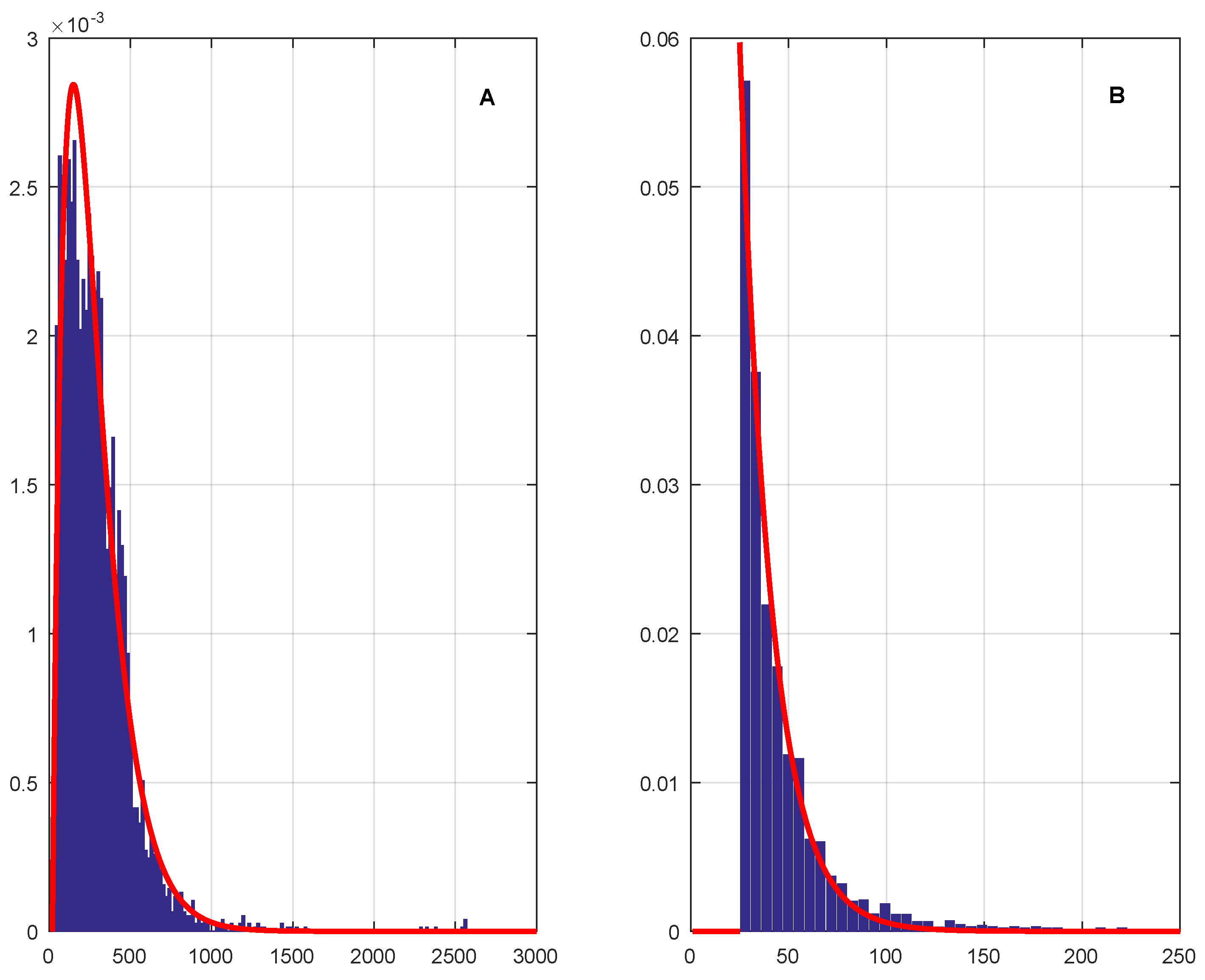
Parameters of the two TNBDs were estimated by minimizing the total variation distance, between the assumed TNBDs and the empirical length distributions for protein-coding genes (model A) and standard noncoding ORFs (model B). The resulting optimal values were for model A and for model B, while the respective minimal total variation distances were found to be and Then, the translation parameters are codons for protein-coding genes and triplets for standard noncoding ORFs. Thus, the best-fitting theoretical length distribution for standard noncoding ORFs is a translated geometric distribution The relatively large magnitude of the minimum total variation distance is due to the fact that many lengths of protein-coding genes and standard noncoding ORFs carrying positive probabilities in the theoretical distributions are absent in the genome of Bacillus subtilis; yet another reason is the presence in this genome of a large number of anomalously long (in relative terms) sequences of both classes.
The profiles of the total variation distance as functions of parameters
p and
q for the optimal values
and
are shown in
Figure 3. Notice that (i) if
or
, then the corresponding theoretical length distributions “escape to infinity” so that
(ii) if
, then
where
is the frequency of the minimum gene length of 20 codons; and (iii) by contrast, if
, then
due to the fact that the shortest length of standard noncoding ORFs is 25 triplets rather than 20 triplets. The limiting behaviors (i)–(iii) are clearly seen in
Figure 3. Finally, the estimated TNBDs and empirical length distributions approximated by suitable histograms are displayed in
Figure 4A,B. We conclude from
Figure 4 that TNBDs with the above-specified parameters provide an excellent visual fit to the empirical length distributions for the two classes of DNA sequences.
For the expected model-based lengths of protein-coding genes and standard noncoding ORFs, measured in triplets, we have
while the corresponding standard deviations, also measured in triplets, are
to be compared with their empirical counterparts
and
A few comments about the length distributions for the two classes of DNA sequences are in order:
- (i)
The genome of Bacillus subtilis contains a large number of very short standard noncoding ORFs. For example, the number of such ORFs with the length of 25 triplets (the shortest possible) is 273, while the number of those with the length ranging from 25 to 30 triplets is 1331 or 29%;
- (ii)
On average, protein-coding genes are much longer than standard noncoding ORFs. In fact, the ratio of their observed average lengths is about 5.4 and that of their model-based expected lengths is about 7.0;
- (iii)
The genome contains a significant number of very long protein-coding genes. The seven longest among them have lengths 3583, 3587, 3603, 4262, 4538, 5043, and 5488 codons, while the eighth longest gene is just 2561 codons long. This explains why the empirical standard deviation of gene length, codons, is substantially larger than its theoretical counterpart, codons. Without the seven longest genes, one would have codons;
- (iv)
Although the number of anomalously long standard noncoding ORFs is disproportionately smaller than the number of very long protein-coding genes, their effect on the standard deviation of the length distribution is still considerable. For example, the longest standard noncoding ORF has 4428 triplets, while the length of the second longest ORF is 1190 triplets. Removing the longest ORF would reduce the standard deviation of ORF length from to 64 triplets.
We also fitted TNBDs to the empirical length distribution for 3283 protein-coding genes beginning with the standard START codon ATG. This resulted in (implying that ) and , while the minimum total variation distance was Thus, the best-fitting TNBD is virtually indistinguishable from the same for the entire set of 4237 Bacillus subtilis protein-coding genes; however, surprisingly, the goodness of fit for the entire collection of genes is even better than for the seemingly more homogeneous subset of genes with the standard START codon ATG. That is why we used the entire set of protein-coding genes in our analysis.
Once models A and B are completely specified, one can evaluate the log-likelihood score
X given by Formula (3) for each DNA sequence from either class. For the above-specified models of sequence length, the first term in (3) for any given sequence of length
is
where
and
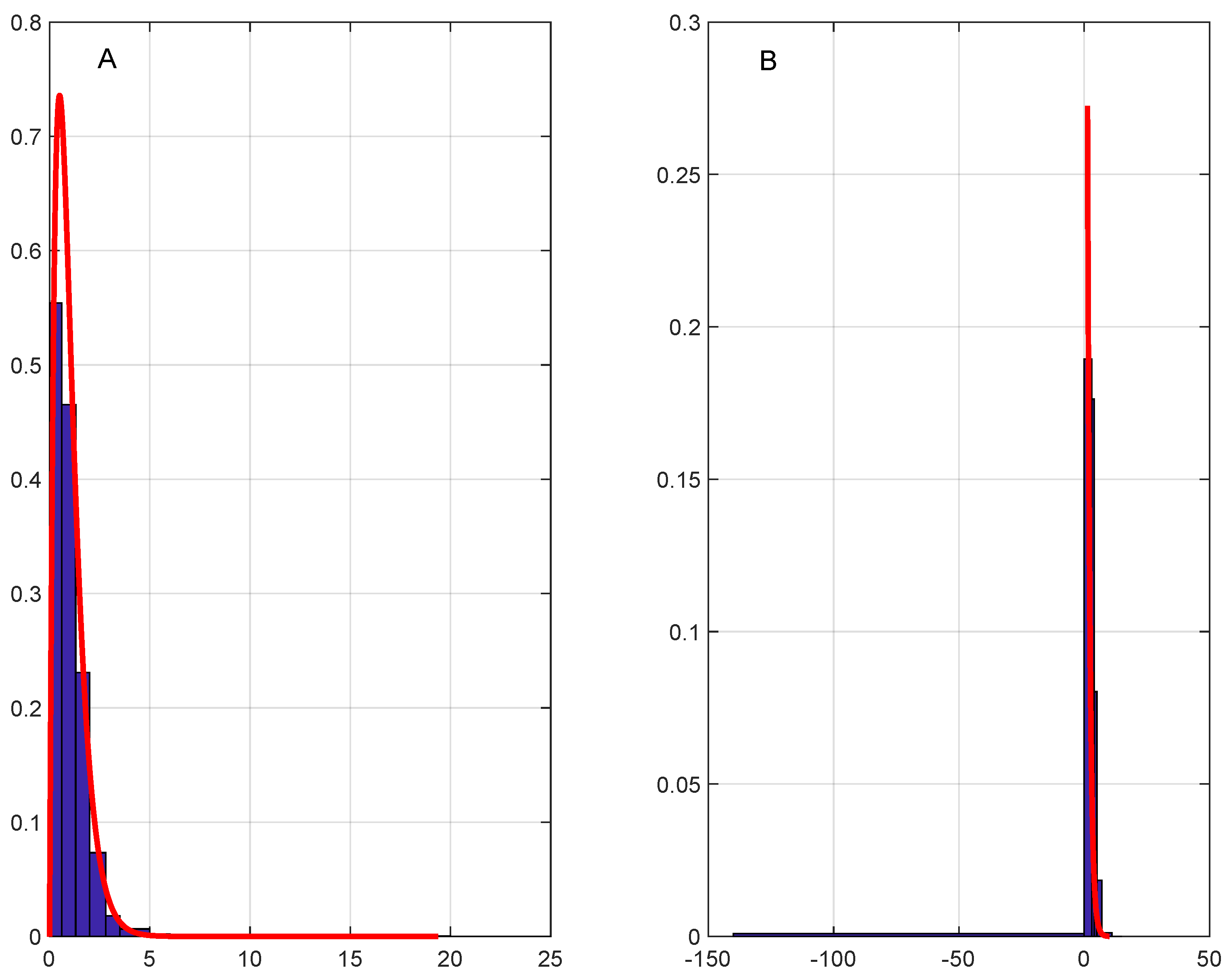
We then computed the class-specific normalized scores
where
and
are sample averages of the log-likelihood score
X over all sequences in the two respective classes, while
and
are the corresponding sample standard deviations. Because the values of parameters
p and
q are small and have roughly the same order of magnitude, it would seem reasonable to compare empirical distributions of the samples
with the respective limiting distributions identified in Theorem 1, see
Figure 5A,B and
Figure 6A,B, where empirical distributions are represented as histograms with appropriately chosen bins. We conclude from
Figure 5 and
Figure 6 that the plain and transformed Erlang distributions found in Theorem 1 reproduce essential features of empirical distributions of the samples
such as range, shape, and mode fairly well.
6. Discussion
In this article, we derived a novel limit theorem for two natural normalizations, and of the log-likelihood score where the expectation and standard deviation are taken relative to either model A or B and it is assumed that the sequence length for these models follows respective TNBDs and The limit theorem applies to long sequences () under the essential additional condition that the expected sequence length for either class is not exponentially larger than for the other class (more precisely, and ). The limiting distributions of rv Y under respective models A and B turned out to be Erlang distributions and , while for rv Z, they came out as transformed Erlang distributions and see Theorem 1. It is noteworthy that the limiting distributions depend on integer parameters a and b alone. Thus, the limiting behavior of the normalized log-likelihood score for long sequences represents, under the assumptions of Theorem 1, a fairly crude phenomenon.
Theorem 1 yields an important corollary: the asymptotic accuracy of the likelihood-based classification of random sequences, see Theorem 2.
To test the utility of our limit theorem, we applied it to the classification of open reading frames (ORFs), see
Section 4, extracted from the genome of the bacterium
Bacillus subtilis strain 168, as protein-coding genes (class A) and standard noncoding ORFs (class B). In this case, the alphabet consists of
triplets of DNA nucleotides other than STOP triplets. Since the genome of
Bacillus subtilis is well annotated, class membership of all ORFs is known with certainty, which allowed us to empirically estimate character selection probabilities and length distributions for both classes of DNA sequences, see
Table 1 and
Figure 4. As was explained in
Section 4, under the model of independent DNA sequence assembly, the length distributions for both classes are mixtures of negative binomial distributions, which we approximated, for each class of sequences, by a single TNBD. The best-fitting distributions from this family provided a surprisingly good fit to the empirical length distributions for both classes of DNA sequences, see
Figure 4. This serves as an indirect validation of our model of DNA sequence assembly. This also corroborates earlier findings that the length of protein-coding genes in many organisms can be approximated by negative binomial distributions [
6] or gamma distributions [
18], which serve as a continuous analog of negative binomial distributions.
The aforementioned (transformed) Erlang distributions with
and
and their empirical counterparts (i.e., the distributions of the observed normalized log-likelihood scores
Y and
Z for the two classes of DNA sequences) are compared in
Figure 5 and
Figure 6. They reveal that the theoretical limiting distributions provide a reasonable fit to the empirical distributions and capture some of their salient features such as range, shape, and mode. This is somewhat unexpected given that (a) the limiting distributions are one-parametric; (b) the model of random independent DNA sequence assembly is quite simplistic; (c) frequencies of the codons immediately following the START codon and immediately preceding the STOP triplet in protein-coding genes are distinct from those for internal codons [
6]; and (d) our model disregards various additional features such as the presence in bacterial genomes of short regulatory nucleotide sequences at characteristic distances from the gene’s START codon including ribosome binding sites (or Shine–Dalgarno sequences) and binding sites for transcription factors [
5,
6].
Our results can be applied to the classification of binary sequences (), DNA sequences viewed at the level of individual nucleotides (), and proteins represented as sequences of amino acids (). They may also potentially have applications in the areas of natural language processing and artificial intelligence.
The principal limitation of this work is the use of an independent (or zero-order Markov chain) model of sequence assembly. It was found long ago that DNA sequences are characterized by the presence of substantial short-range [
7] and long-range [
8] correlations between nucleotides and their triplets. As a result, efficient modern methods of computational gene finding employ higher-order, or even variable-order, Markov chain models and Hidden Markov models at the level of individual nucleotides [
4,
5,
6]. For example, a gene finder called GeneMark [
5] employs a 5th-order Markov chain model, while GLIMMER gene finder [
4] combines
k-th order Markov chain models for
Although the accuracy of gene finding generally increases with
k (the order of the Markov chain), the use of large values of
k is prohibited by the large number,
of Markov transition probabilities that have to be estimated from a training set and the sparsity of
− tuples of nucleotides used for estimation purposes. Thus, to make our limit theorem a better discriminator between protein-coding genes and noncoding ORFs in prokaryotic genomes, it should be extended to higher-order Markov chain models and Hidden Markov models of DNA sequence assembly, and to more general sequence length distributions including translated mixtures of negative binomial distributions.
On the mathematical side, our limit theorem would be more practical if augmented with a tight estimate of the Zolotarev metric [
9,
14] or another suitable distance [
19] between the empirical distribution of the normalized log-likelihood score and its theoretical limiting counterpart.


