
Dual-Domain Image Encryption in Unsecure Medium—A Secure Communication Perspective

 ,
, 
Abstract
1. Introduction
- The usage of lift wavelet transform as the intermediate stage of the ciphering process to effectively reduce the operational time;
- The development of a hybrid chaotic system to offer high keyspace;
- The design of bit-level diffusion to break the pixel dependencies.
2. Background
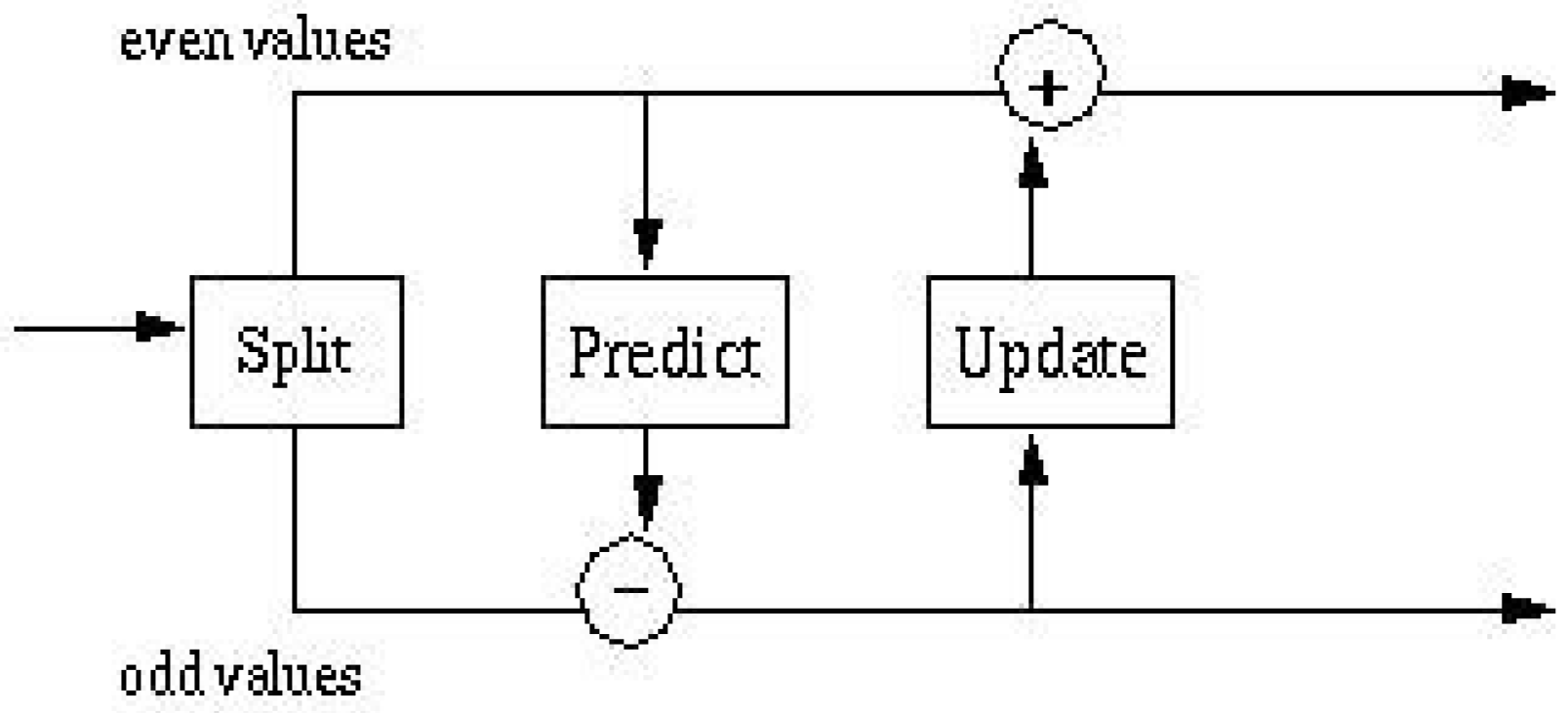
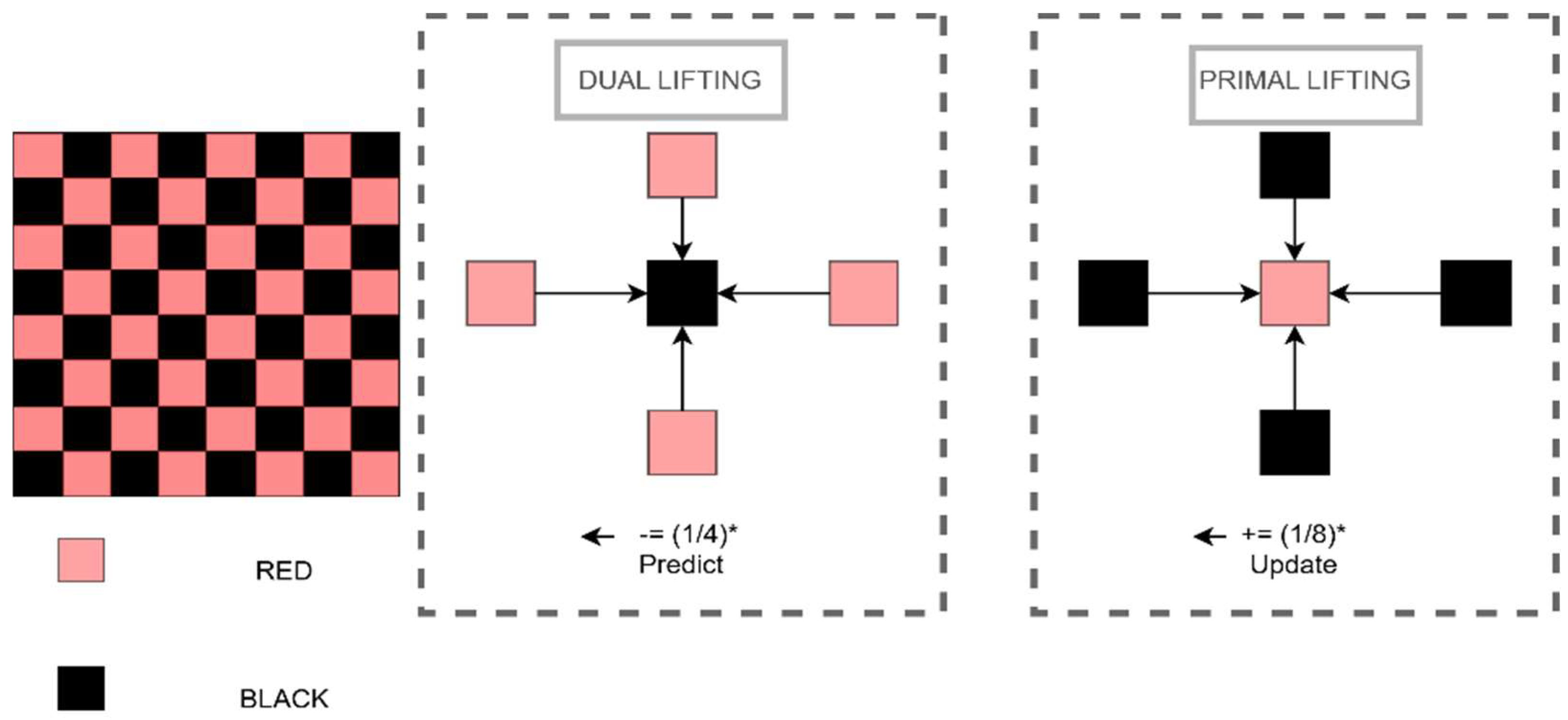
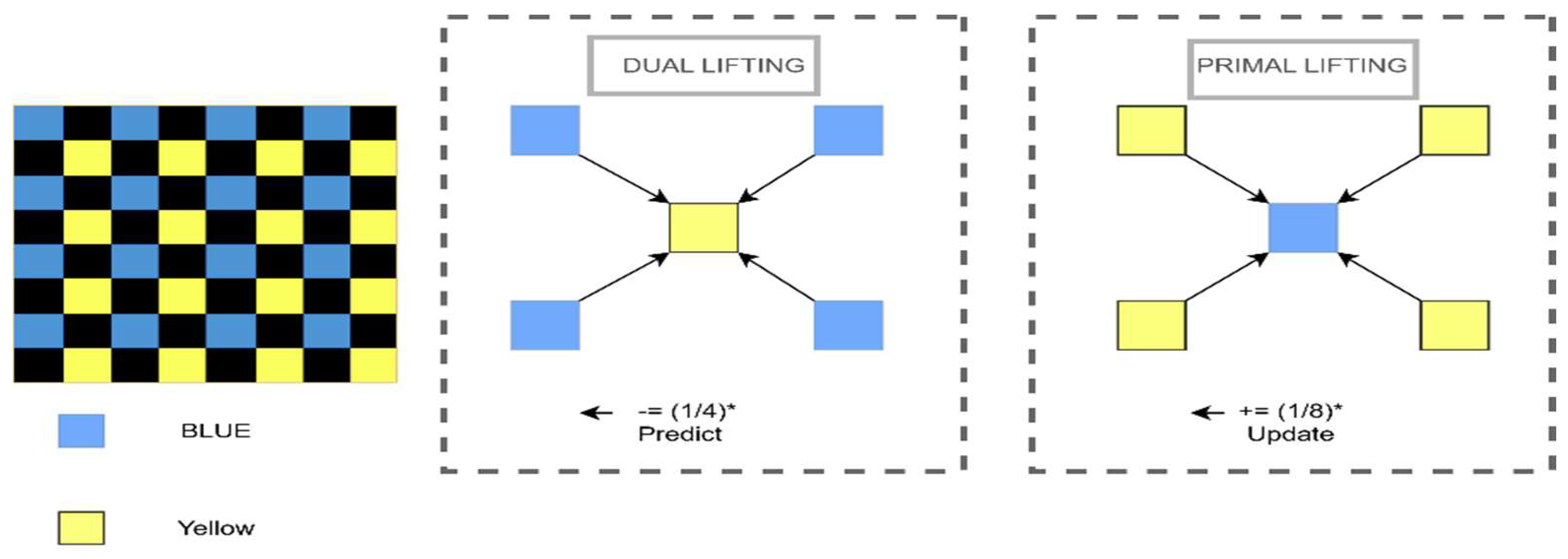
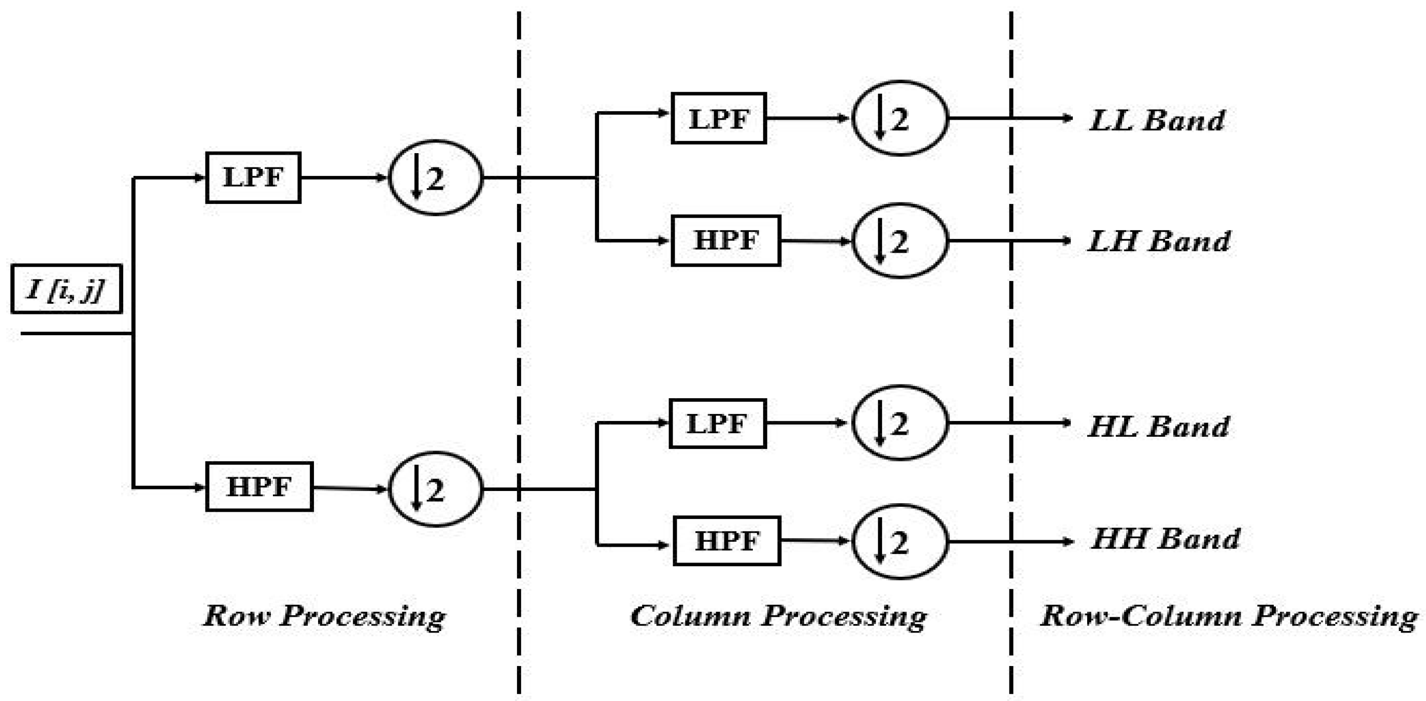
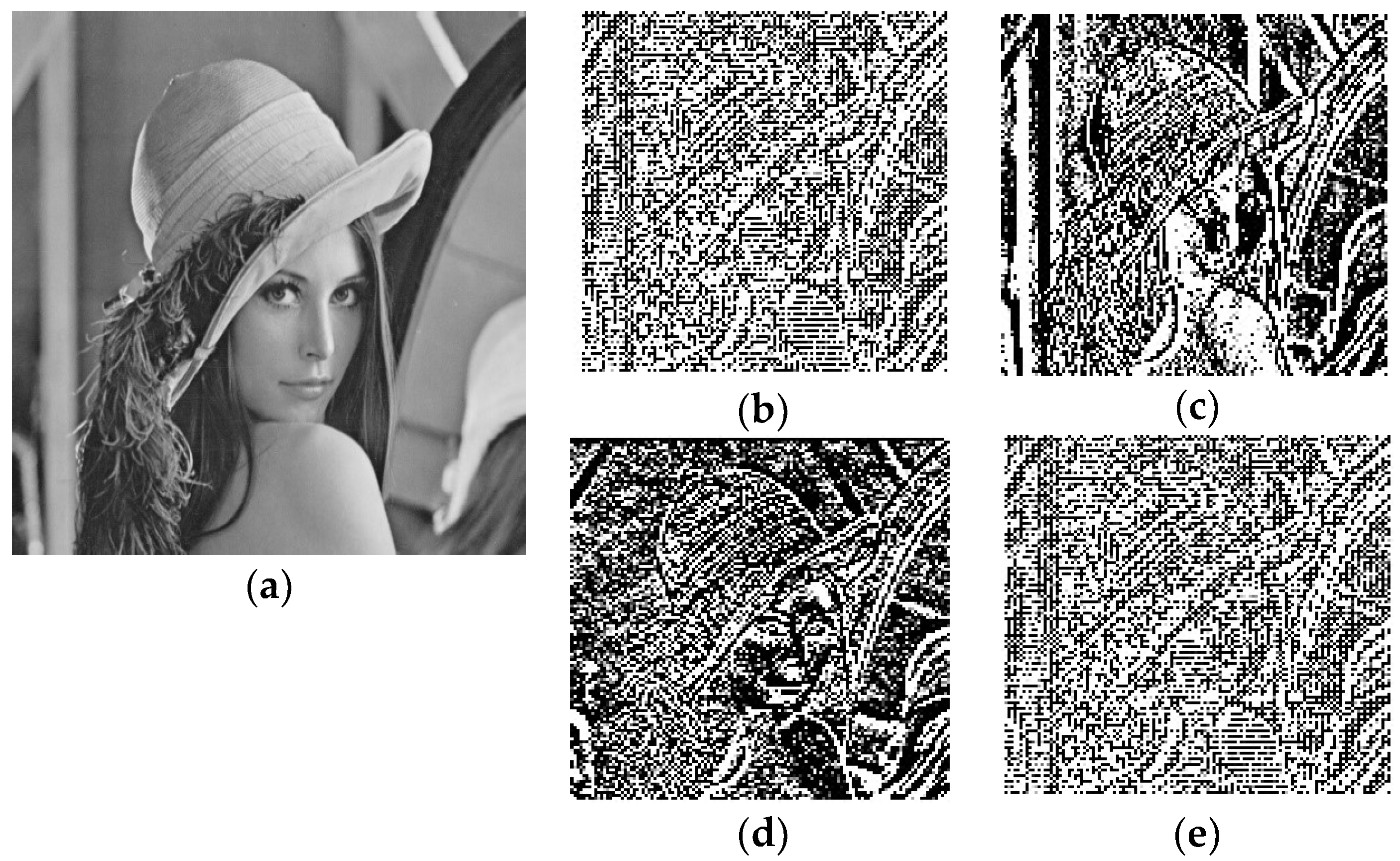
2.1. Lifting Wavelet Transform
2.1.1. Split
2.1.2. Predict
2.1.3. Update
2.2. Chaotic Maps
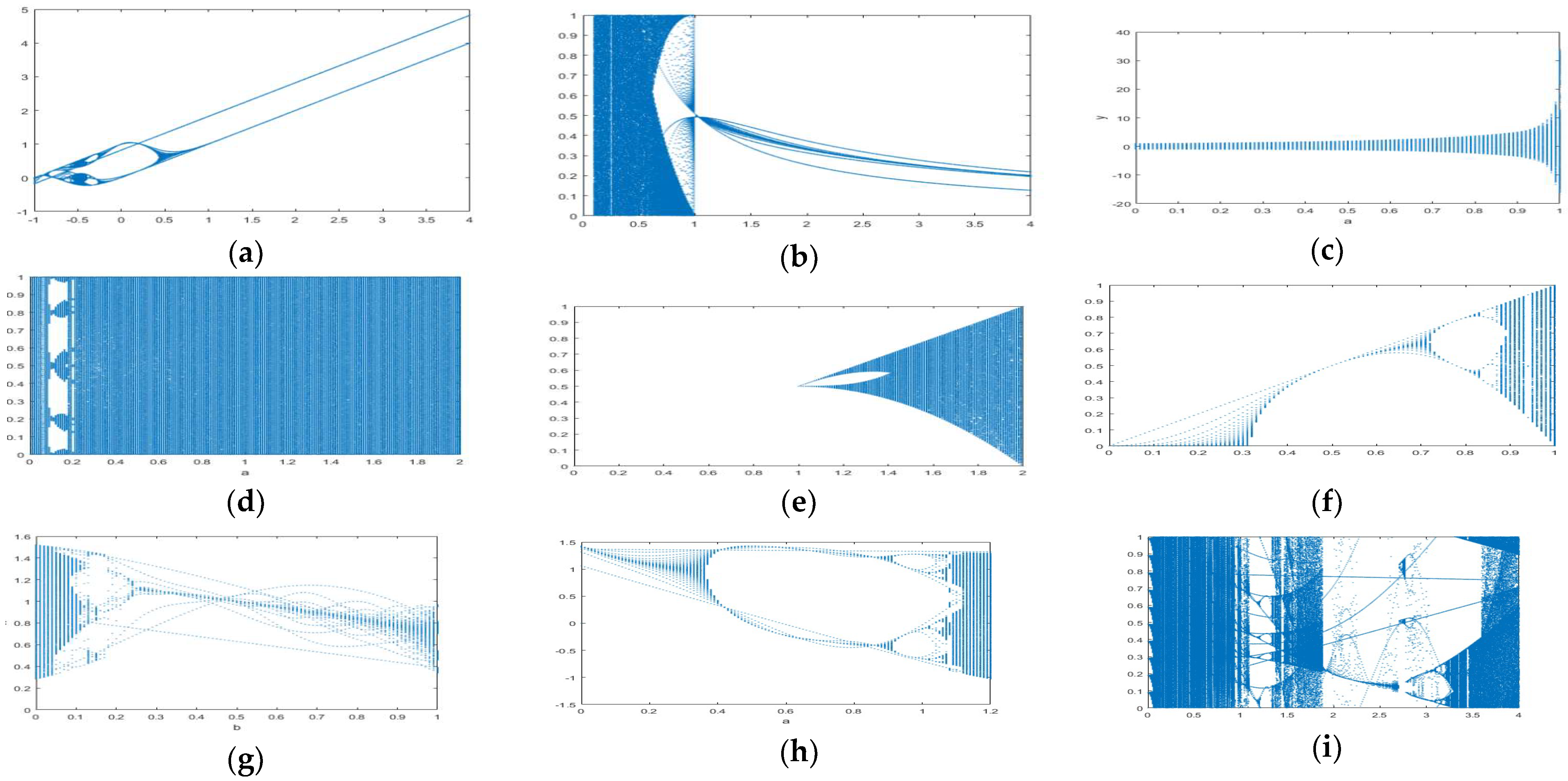
2.2.1. Kaplan–Yorke Map
2.2.2. Gauss Map
2.2.3. Piecewise Linear Map
2.2.4. Chirikov–Taylor Map
2.2.5. Tent Map
2.2.6. Sine Map
2.2.7. Duffing Map
2.2.8. Henon Map
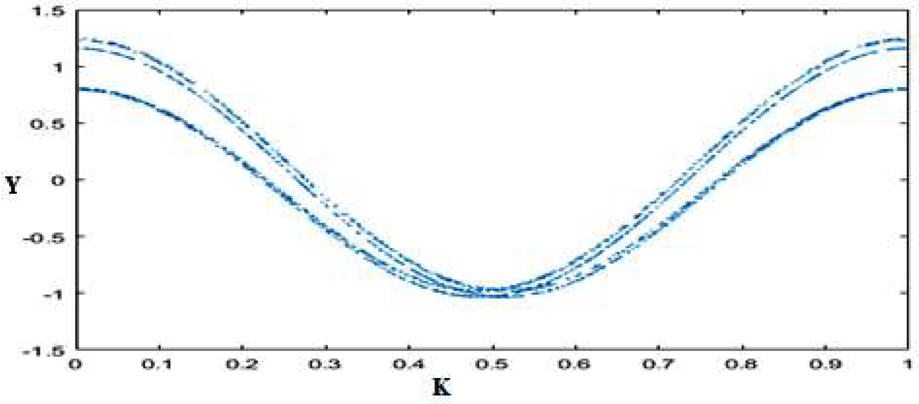
2.2.9. Circle Map
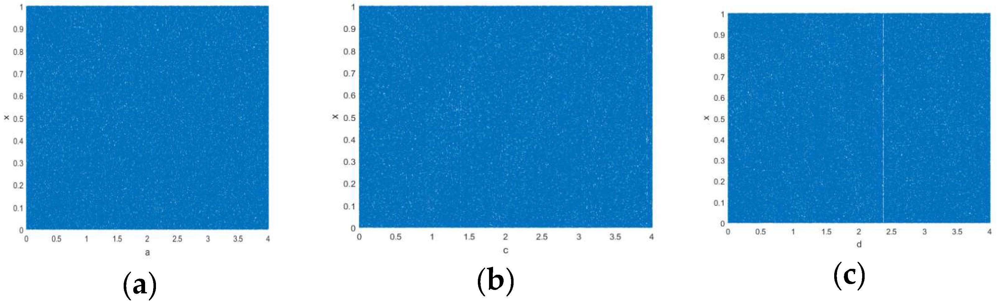
3. Proposed Hybrid Chaotic Map
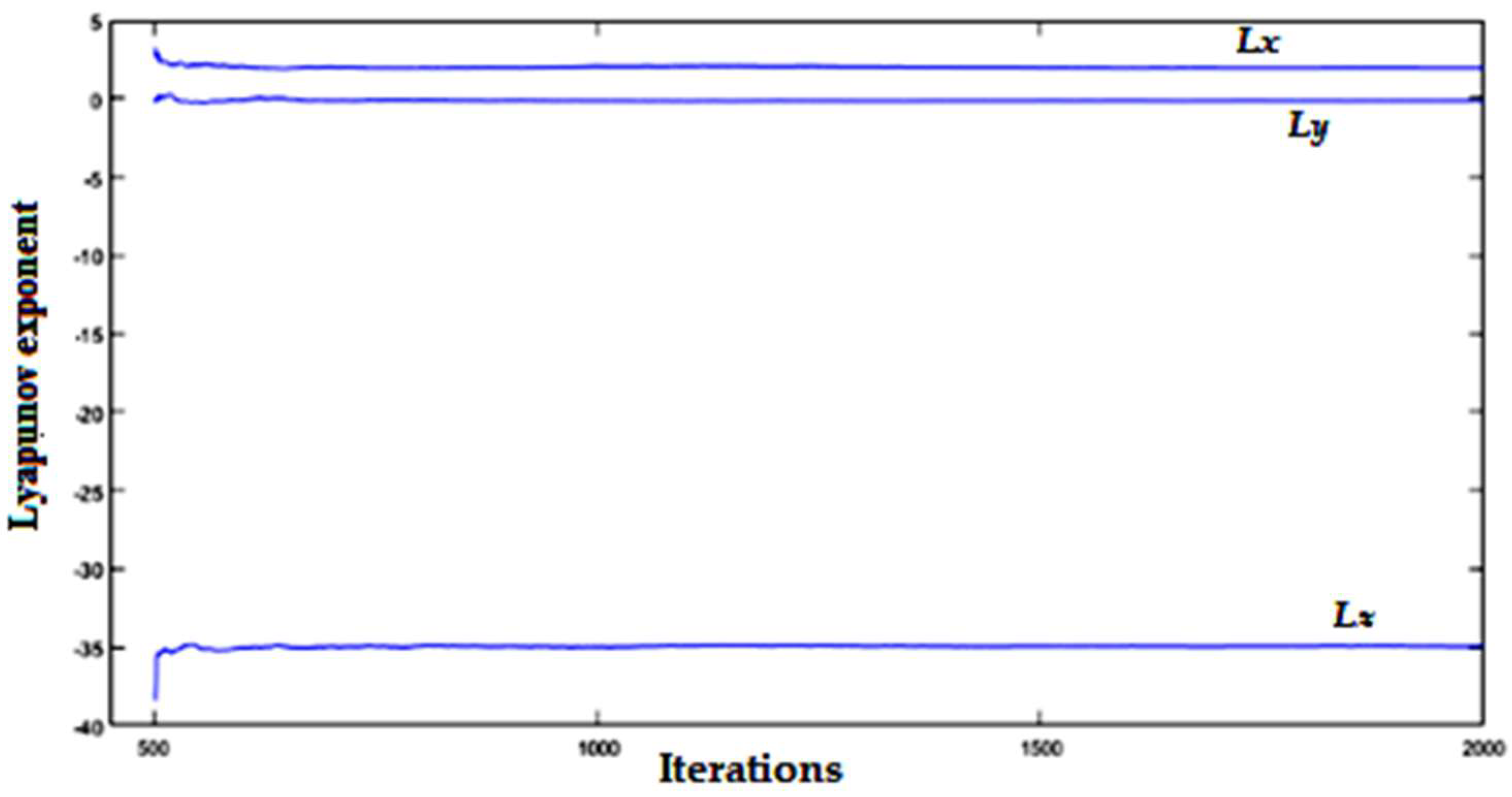
3.1. Lyapunov Exponents for Proposed Map
3.2. Choosing Initial Value for Chaotic Maps
4. Proposed Methodology
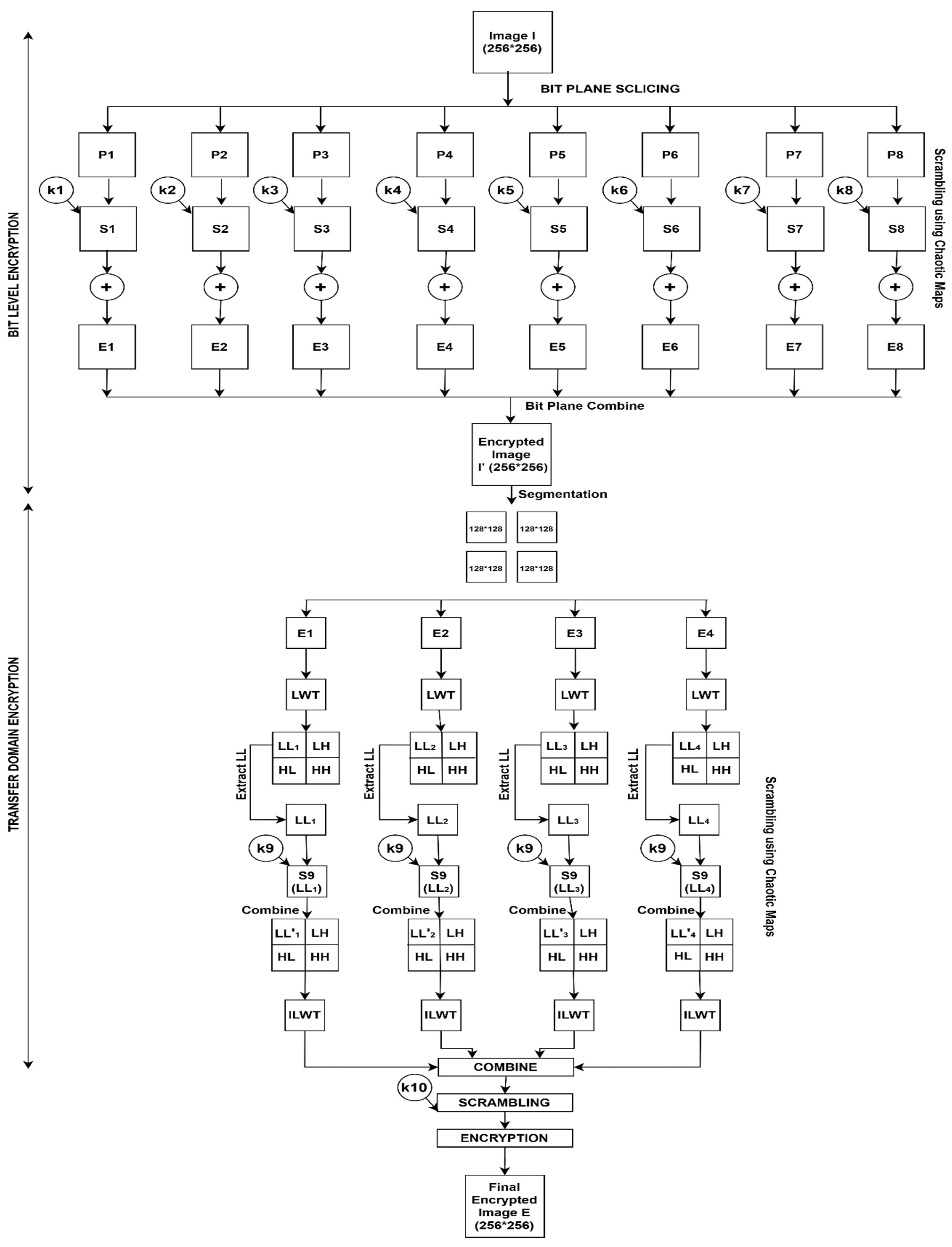
4.1. Encryption
| Algorithm 1 Encryption |
| Input: the 8-bit grayscale image of size 256 × 256 Output: the encrypted image of size 256 × 256 Step 1: Take an input image I and slice the image into constituent bit planes. For an 8-bit image, 8-bit planes will be formed. Step 2: Determine the initial values of the chaotic maps from Section 3.2. Step 3: For each sliced bit plane:
Step 4: Recombine encrypted planes to form I′. Step 5: Divide I′ into four parts, E1, E2, E3, and E4, each of size 128 × 128. Step 6: For each of the four sub-parts of size 128 × 128, perform the following operations:
Step 8: The final layer of scrambling is done using the proposed Hybrid Chaotic map, whose initial value is found using equations in Section 3.2. Step 9: Generate a key using step 3(d) using values in the range of 0–255 instead of in the range 0–1. Step 10: The generated key from step 9 is XORed with R to give the final encrypted image E. |
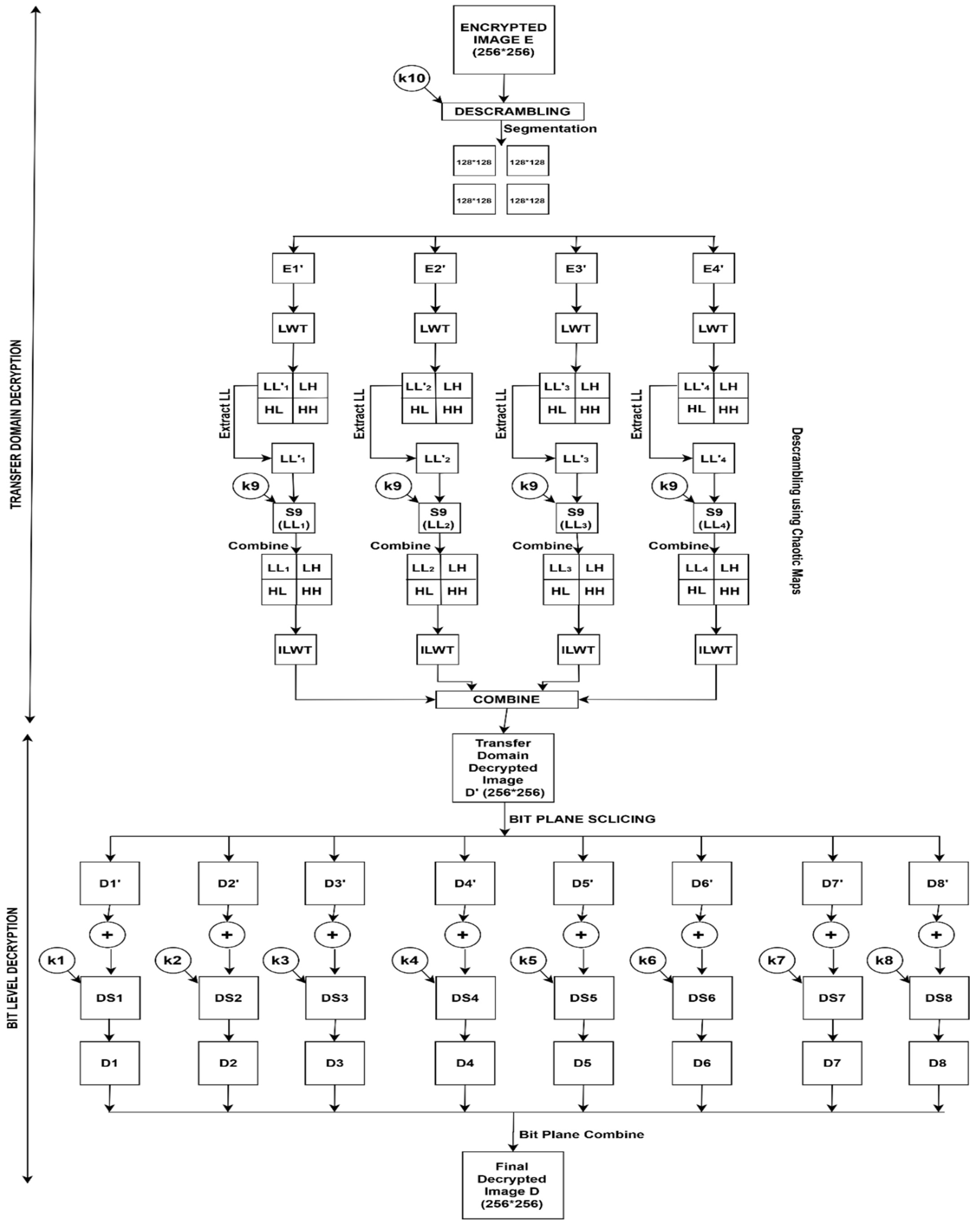
4.2. Decryption
| Algorithm 2 Decryption |
| Input: the encrypted image of size 256 × 256 Output: the 8-bit grayscale image of size 256 × 256 Step 1: Encrypted image E is XORed with the key used in the final encryption layer. Step 2: Descramble the image using the same hybrid chaotic map. The pixels corresponding to the sorted generated chaotic array are placed in the positions corresponding to the indices of the sorted values in the generated unsorted 1D chaotic array to give E′. Step 3: Divide E′ into four parts, E1’, E2′, E3′ and E4′ Step 4: For each subpart E1’, E2′, E3′ and E4′:
Step 6: Slice new D′ into constituent bit planes. Step 7: For each bit plane:
|
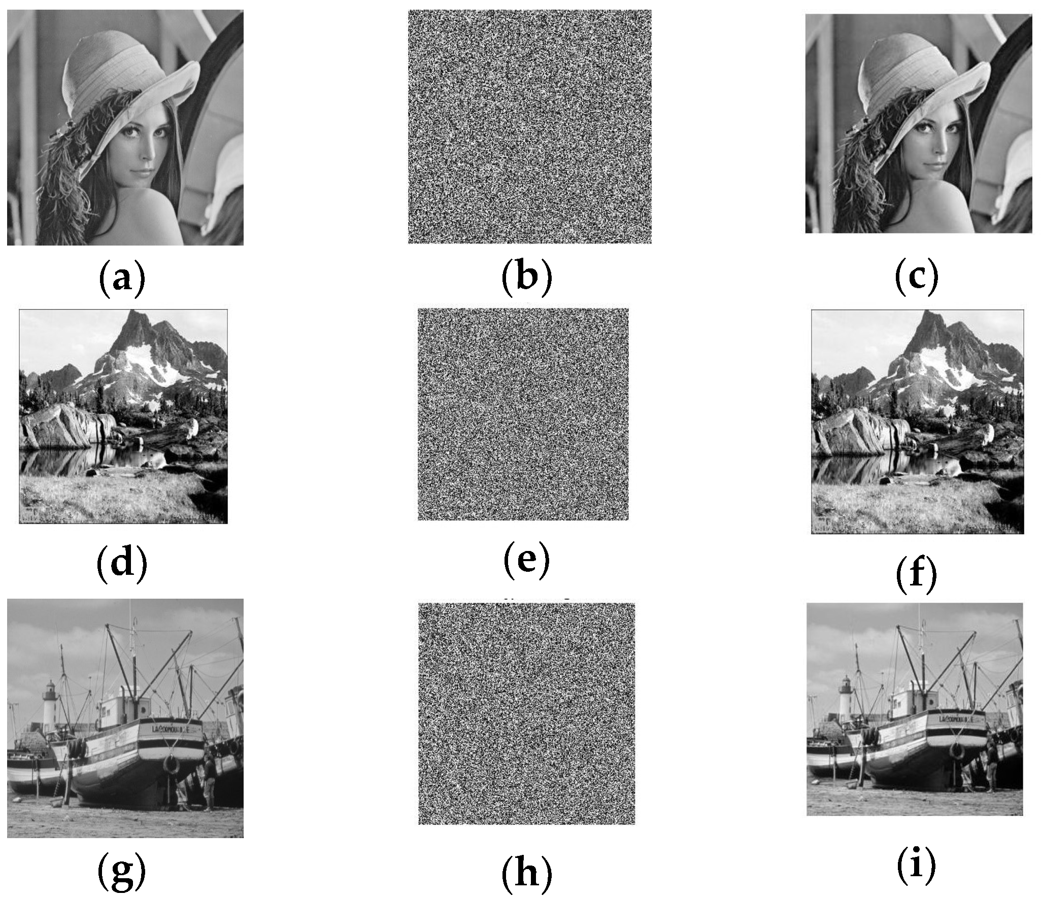
5. Results and Performance Measures
5.1. Statistical Analysis
5.1.1. MSE, PSNR, and SSIM
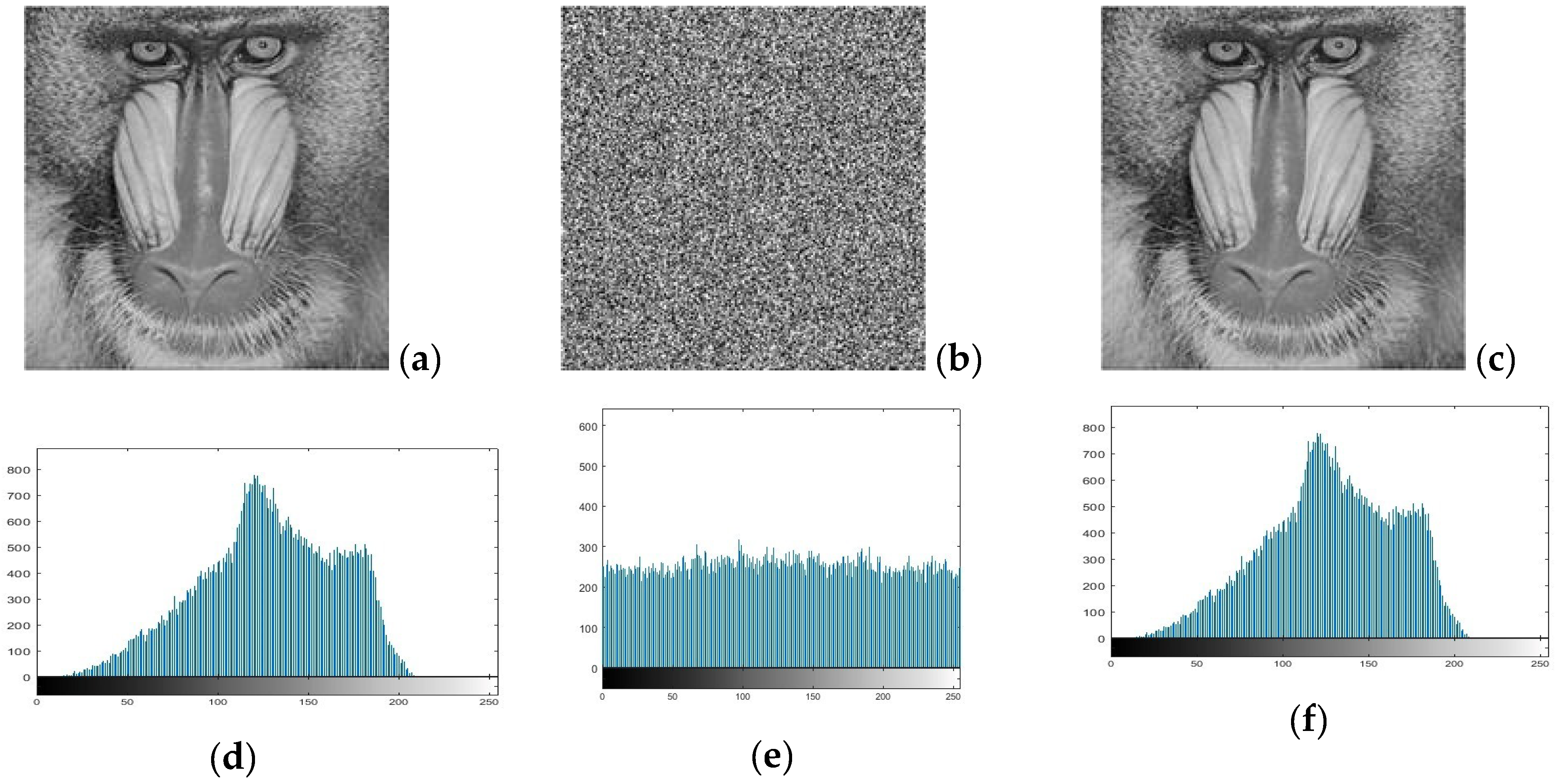
5.1.2. Histogram Analysis
5.1.3. Information Entropy
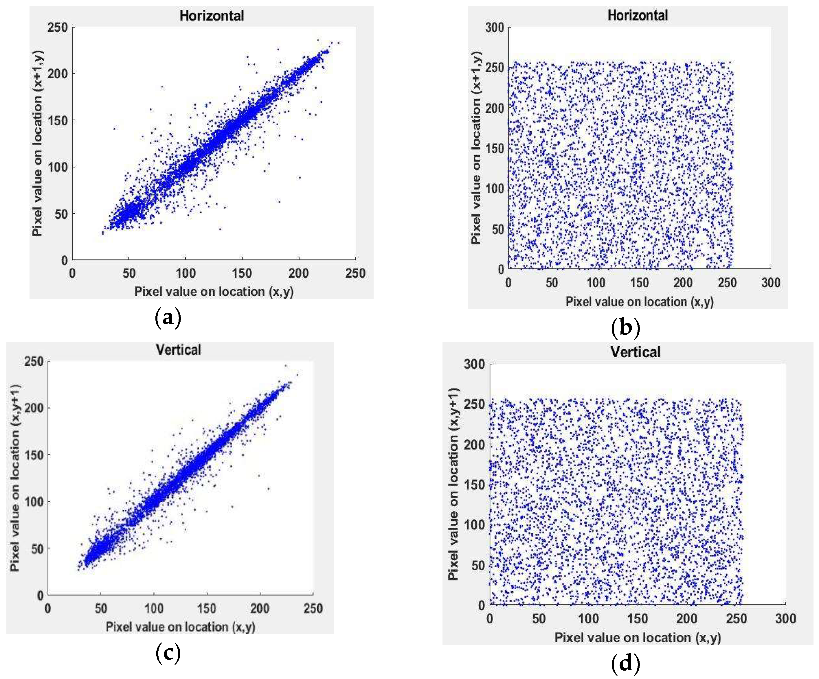
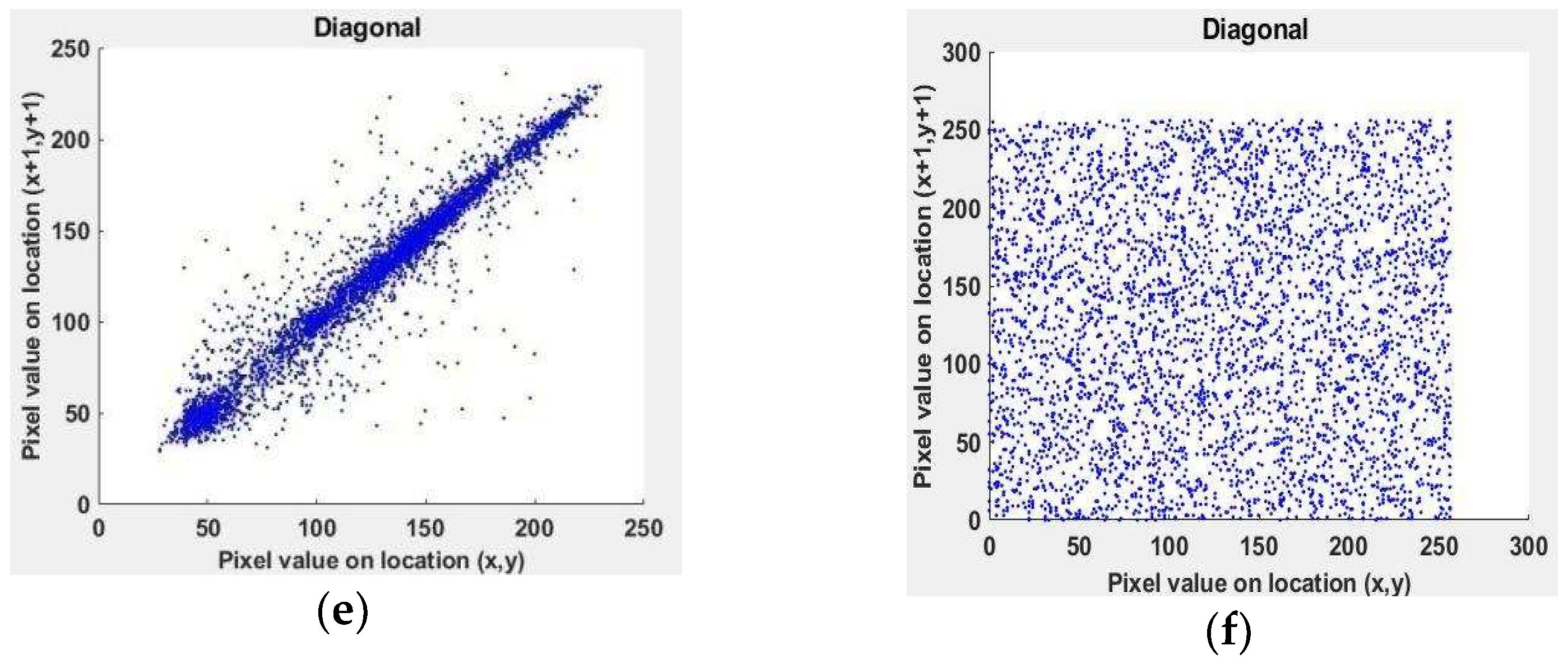
5.1.4. Correlation Test
5.2. Differential Attack Analysis
5.3. Key Space Analysis and Key Sensitivity
5.4. Robustness
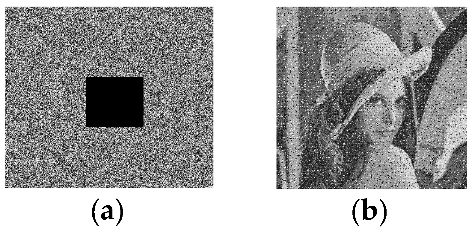
5.4.1. Cropping Attack
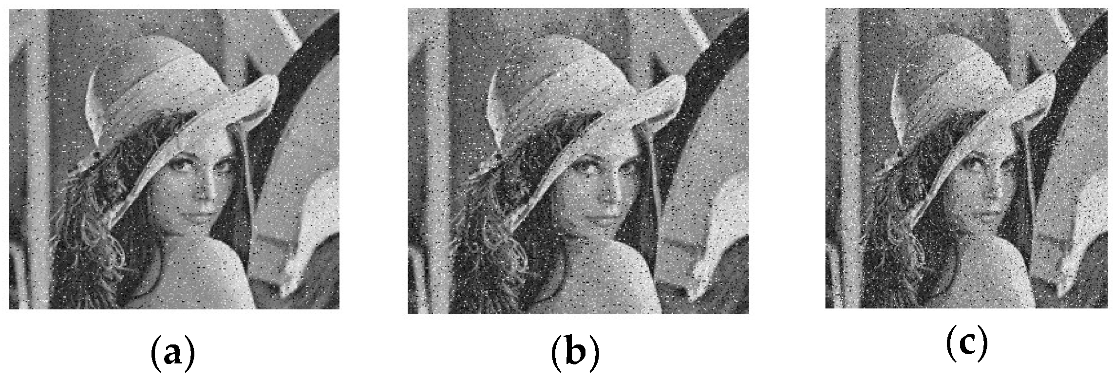
5.4.2. Noise Attack
5.5. Computational Complexity
5.6. NIST SP 800-22
6. Discussion of the Obtained Results
- A hybrid chaotic system-driven cryptosystem was developed;
- Lifting wavelet transform decomposition was adopted to achieve quantization error-free frequency separation;
- Bit plane-based diffusion was used to break the pixel dependency in an effective way which resulted in a near-zero correlation on encrypted pixels;
- Ten different keys were used to accomplish the encryption through which the keyspace was increased to 1.044 × 2184;
- Segmentation of the intermediate cipher image helped to reduce the time consumption, which resulted in a time of 2.1743 s to encrypt a 256 × 256 × 8-bit image;
- A maximum entropy of 7.9972 was achieved with an average PSNR of 8.84139.
7. Conclusions
Author Contributions
Funding
Data Availability Statement
Acknowledgments
Conflicts of Interest
References
- Khan, M.; Shah, T. A Literature Review on Image Encryption Techniques. 3D Res. 2014, 5, 29. [Google Scholar] [CrossRef]
- Kaur, M.; Kumar, V. A Comprehensive Review on Image Encryption Techniques. Arch. Comput. Methods Eng. 2018, 27, 15–43. [Google Scholar] [CrossRef]
- Jung, H. Data hiding scheme improving embedding capacity using mixed PVD and LSB on bit plane. J. Real-Time Image Process. 2018, 14, 127–136. [Google Scholar] [CrossRef]
- Huang, H.-Y.; Chang, S.-H. A Lossless Data Hiding based on Discrete Haar Wavelet Transform. In Proceedings of the IEEE International Conference on Computer and Information Technology, Bradford, UK, 29 June–1 July 2010; pp. 1554–1559. [Google Scholar]
- Tedmori, S.; Al-Najdawi, N. Image cryptographic algorithm based on the Haar wavelet transform. Inf. Sci. 2014, 269, 21–34. [Google Scholar] [CrossRef]
- Li, C.; Lin, D.; Lu, J. Cryptanalyzing an Image-Scrambling Encryption Algorithm of Pixel Bits. IEEE MultiMedia 2017, 24, 64–71. [Google Scholar] [CrossRef]
- Hua, Z.; Zhou, B.; Zhou, Y. Sine-Transform-Based Chaotic System with FPGA Implementation. IEEE Trans. Ind. Electron. 2018, 65, 2557–2566. [Google Scholar] [CrossRef]
- Suneja, K.; Dua, S.; Dua, M. A Review of Chaos based Image Encryption. In Proceedings of the International Conference on Computing Method-Ologies and Communication (ICCMC), Erode, India, 27–29 March 2019; pp. 693–698. [Google Scholar]
- Hua, Z.; Zhou, Y. One-Dimensional Nonlinear Model for Producing Chaos. IEEE Trans. Circuits Syst. I Regul. Pap. 2017, 65, 235–246. [Google Scholar] [CrossRef]
- Gao, S.; Wu, R.; Wang, X.; Wang, J.; Li, Q.; Wang, C.; Tang, X. A 3D model encryption scheme based on a cascaded chaotic system. Signal Process. 2023, 202, 108745. [Google Scholar] [CrossRef]
- Zhu, H.; Zhao, Y.; Song, Y. 2D Logistic-Modulated-Sine-Coupling-Logistic Chaotic Map for Image Encryption. IEEE Access 2019, 7, 14081–14098. [Google Scholar] [CrossRef]
- Tang, Z.; Yang, Y.; Xu, S.; Yu, C.; Zhang, X. Image Encryption with Double Spiral Scans and Chaotic Maps. J. Secur. Commun. Netw. 2019, 2019, 8694678. [Google Scholar] [CrossRef]
- Ye, G.; Huang, X. A secure image encryption algorithm based on chaotic maps and SHA-3. J. Secur. Commun. Netw. 2016, 9, 2015–2023. [Google Scholar] [CrossRef]
- Agarwal, S. A Review of Image Scrambling Technique Using Chaotic Maps. Int. J. Eng. Technol. Innov. 2018, 8, 77–98. [Google Scholar]
- Sankpal, P.R.; Vijaya, P.A. Image Encryption Using Chaotic Maps: A Survey. In Proceedings of the 2014 Fifth International Conference on Signals and Image, Cherbourg, France, 20 June–2 July 2014; IEEE Conference Publication: Cherbourg, France, 2014. [Google Scholar]
- Abdullah, H.N.; Abdullah, H.A. Image encryption using hybrid chaotic map. In Proceedings of the 2017 International Conference on Current Research in Computer Science and Information Technology (ICCIT), Dhaka, Bangladesh, 22–24 December 2017; pp. 121–125. [Google Scholar]
- Banu, S.A.; Amirtharajan, R. A robust medical image encryption in dual domain: Chaos-DNA-IWT combined approach. Med. Biol. Eng. Comput. 2020, 58, 1445–1458. [Google Scholar] [CrossRef] [PubMed]
- Rajini, G.K. A Comprehensive Review on Wavelet Transform and Its Applications. 2016. Available online: http://www.arpnjournals.org/jeas/research_papers/rp_2016/jeas_1016_5133.pdf (accessed on 10 December 2022).
- Uytterhoeven, G.; Roose, D.; Bultheel, A. Wavelet Transforms Using the Lifting Scheme. ITA-Wavelets Report WP, 1. 1997. Available online: https://citeseerx.ist.psu.edu/document?repid=rep1&type=pdf&doi=e154fe1bf4777fcad4bc70a7e01611e7a5c43e9c (accessed on 10 December 2022).
- Luo, Y.; Wang, F.; Xu, S.; Zhang, S.; Li, L.; Su, M.; Liu, J. CONCEAL: A robust dual-color image watermarking scheme. Expert Syst. Appl. 2022, 208, 118133. [Google Scholar] [CrossRef]
- Singh, S.P.; Bhatnagar, G. A simplified watermarking algorithm based on lifting wavelet transform. Multimed. Tools Appl. 2019, 78, 20765–20786. [Google Scholar] [CrossRef]
- Jan, A.; Parah, S.A.; Hussan, M.; Malik, B.A. Double layer security using crypto-stego techniques: A comprehensive review. Health Technol. 2021, 12, 9–31. [Google Scholar] [CrossRef]
- Salunke, S.; Ahuja, B.; Hashmi, M.F.; Marriboyina, V.; Bokde, N.D. 5D Gauss Map Perspective to Image Encryption with Transfer Learning Validation. Appl. Sci. 2022, 12, 5321. [Google Scholar] [CrossRef]
- Li, C.; Luo, G.; Qin, K.; Li, C. An image encryption scheme based on chaotic tent map. Nonlinear Dyn. 2016, 87, 127–133. [Google Scholar] [CrossRef]
- Hua, Z.; Zhou, Y. Image encryption using 2D Logistic-adjusted-Sine map. Inf. Sci. 2016, 339, 237–253. [Google Scholar] [CrossRef]
- Khan, M.; Masood, F. A novel chaotic image encryption technique based on multiple discrete dynamical maps. Multimed. Tools Appl. 2019, 78, 26203–26222. [Google Scholar] [CrossRef]
- Rakheja, P.; Yadav, S.; Tobria, A. A novel image encryption mechanism based on umbrella map and Yang-Gu algorithm. Optik 2022, 271, 170152. [Google Scholar] [CrossRef]
- Banu, S.A.; Amirtharajan, R. Tri-level scrambling and enhanced diffusion for DICOM image cipher-DNA and chaotic fused approach. Multimed. Tools Appl. 2020, 79, 28807–28824. [Google Scholar] [CrossRef]
- Banu, S.A.; Amirtharajan, R. Bio-inspired cryptosystem on the reciprocal domain: DNA strands mutate to secure health data. Front. Inf. Technol. Electron. Eng. 2021, 22, 940–956. [Google Scholar] [CrossRef]
- Chen, Y.; Tang, C.; Ye, R. Cryptanalysis and improvement of medical image encryption using high-speed scrambling and pixel adaptive diffusion. Signal Process. 2019, 167, 107286. [Google Scholar] [CrossRef]
- Guan, M.; Yang, X.; Hu, W. Chaotic image encryption algorithm using frequency-domain DNA encoding. IET Image Process. 2019, 13, 1535–1539. [Google Scholar] [CrossRef]
- Belazi, A.; Talha, M.; Kharbech, S.; Xiang, W. Novel Medical Image Encryption Scheme Based on Chaos and DNA Encoding. IEEE Access 2019, 7, 36667–36681. [Google Scholar] [CrossRef]
- Haghighi, B.B.; Taherinia, A.H.; Mohajerzadeh, A.H. TRLG: Fragile blind quad watermarking for image tamper detection and recovery by providing compact digests with optimized quality using LWT and GA. Inf. Sci. 2019, 486, 204–230. [Google Scholar] [CrossRef]
- Stalin, S.; Maheshwary, P.; Shukla, P.K.; Maheshwari, M.; Gour, B.; Khare, A. Fast and Secure Medical Image Encryption Based on Non Linear 4D Logistic Map and DNA Sequences (NL4DLM_DNA). J. Med. Syst. 2019, 43, 267. [Google Scholar] [CrossRef]
- Liu, T.; Banerjee, S.; Yan, H.; Mou, J. Dynamical analysis of the improper fractional-order 2D-SCLMM and its DSP implementation. Eur. Phys. J. Plus 2021, 136, 506. [Google Scholar] [CrossRef]
- Liu, T.; Yan, H.; Banerjee, S.; Mou, J. A fractional-order chaotic system with hidden attractor and self-excited attractor and its DSP implementation. Chaos Solitons Fractals 2021, 145, 110791. [Google Scholar] [CrossRef]
- Kaur, G.; Agarwal, R.; Patidar, V. Color image encryption system using combination of robust chaos and chaotic order fractional Hartley transformation. J. King Saud Univ. Comput. Inf. Sci. 2022, 34, 5883–5897. [Google Scholar] [CrossRef]
- Yang, F.; Mou, J.; Ma, C.; Cao, Y. Dynamic analysis of an improper fractional-order laser chaotic system and its image en-cryption application. Opt. Lasers Eng. 2020, 129, 106031. [Google Scholar] [CrossRef]
- Zefreh, E.Z. An image encryption scheme based on a hybrid model of DNA computing, chaotic systems and hash functions. Multimed. Tools Appl. 2020, 79, 24993–25022. [Google Scholar] [CrossRef]
- Zhang, X.; Hu, Y. Multiple-image encryption algorithm based on the 3D scrambling model and dynamic DNA coding. Opt. Laser Technol. 2021, 141, 107073. [Google Scholar] [CrossRef]
- Ravichandran, D.; Banu, S.A.; Murthy, B.; Balasubramanian, V.; Fathima, S.; Amirtharajan, R. An efficient medical image encryption using hybrid DNA computing and chaos in transform domain. Med. Biol. Eng. Comput. 2021, 59, 589–605. [Google Scholar] [CrossRef] [PubMed]
- Patel, S.; Thanikaiselvan, V.; Pelusi, D.; Nagaraj, B.; Arunkumar, R.; Amirtharajan, R. Colour image encryption based on customized neural network and DNA encoding. Neural Comput. Appl. 2021, 33, 14533–14550. [Google Scholar] [CrossRef]
- Zheng, J.; Liu, L. Novel image encryption by combining dynamic DNA sequence encryption and the improved 2D logistic sine map. IET Image Process. 2020, 14, 2310–2320. [Google Scholar] [CrossRef]
- Li, J.; Chen, L.; Cai, W.; Xiao, J.; Zhu, J.; Hu, Y.; Wen, K. Holographic encryption algorithm based on bit-plane decomposition and hyperchaotic Lorenz system. Opt. Laser Technol. 2022, 152, 108127. [Google Scholar] [CrossRef]
- Zhang, F.; Zhang, X.; Cao, M.; Ma, F.; Li, Z. Characteristic Analysis of 2D Lag-Complex Logistic Map and Its Application in Image Encryption. IEEE MultiMedia 2021, 28, 96–106. [Google Scholar] [CrossRef]
- Lone, M.A.; Qureshi, S. RGB image encryption based on symmetric keys using Arnold transform, 3D chaotic map and affine hill cipher. Optik 2022, 260, 168880. [Google Scholar] [CrossRef]
- Teng, L.; Wang, X.; Xian, Y. Image encryption algorithm based on a 2D-CLSS hyperchaotic map using simultaneous permutation and diffusion. Inf. Sci. 2022, 605, 71–85. [Google Scholar] [CrossRef]
- Ye, G.; Wu, H.; Liu, M.; Shi, Y. Image encryption scheme based on blind signature and an improved Lorenz system. Expert Syst. Appl. 2022, 205, 117709. [Google Scholar] [CrossRef]
- Sridevi, A.; Sivaraman, R.; Balasubramaniam, V.; Sreenithi; Siva, J.; Thanikaiselvan, V.; Rengarajan, A. On Chaos based duo confusion duo diffusion for colour images. Multimed. Tools Appl. 2022, 81, 16987–17014. [Google Scholar] [CrossRef]
- Zhang, Y.; Xie, H.; Sun, J.; Zhang, H. An efficient multi-level encryption scheme for stereoscopic medical images based on coupled chaotic system and Otsu threshold segmentation. Comput. Biol. Med. 2022, 146, 105542. [Google Scholar] [CrossRef] [PubMed]
- Tutueva, A.; Nepomuceno, E.G.; Moysis, L.; Volos, C.; Butusov, D. Adaptive Chaotic Maps in Cryptography Applications. In Cybersecurity. Studies in Big Data; Abd El-Latif, A.A., Volos, C., Eds.; Springer: Cham, Switzerland, 2022; Volume 102. [Google Scholar] [CrossRef]
- Tutueva, A.V.; Moysis, L.; Rybin, V.G.; Kopets, E.E.; Volos, C.; Butusov, D.N. Fast synchronization of symmetric Hénon maps using adaptive symmetry control. Chaos Solitons Fractals 2022, 155, 111732. [Google Scholar] [CrossRef]
- Anushiadevi, R.; Amirtharajan, R. Separable reversible data hiding in an encrypted image using the adjacency pixel difference histogram. J. Inf. Secur. Appl. 2023, 72, 103407. [Google Scholar] [CrossRef]
- Zhang, X.; Wang, X. Multiple-image encryption algorithm based on DNA encoding and chaotic system. Multimed. Tools Appl. 2018, 78, 7841–7869. [Google Scholar] [CrossRef]


| S. No. | Image | MSE | PSNR (in dB) | SSIM |
|---|---|---|---|---|
| 1. | Lena | 7734.48 | 9.2465 | 0.0124 |
| 2. | Barb | 7666.37 | 9.2849 | 0.0120 |
| 3. | Boat | 8232.87 | 8.9753 | 0.0088 |
| 4. | Goldhill | 8009.06 | 9.0950 | 0.0120 |
| 5. | Mandrill | 6929.84 | 9.7236 | 0.0105 |
| 6. | Mountain | 11,140.38 | 7.6618 | 0.0114 |
| 7. | Washsat | 9365.16 | 8.4156 | 0.0094 |
| 8. | Peppers | 9255.63 | 8.4667 | 0.0090 |
| 9. | Cameraman | 9412.01 | 8.3940 | 0.0092 |
| 10. | Pirate | 7907.29 | 9.1505 | 0.0110 |
| S. No. | Image | Entropy |
|---|---|---|
| 1. | Lena | 7.9976 |
| 2. | Barb | 7.9974 |
| 3. | Boat | 7.9970 |
| 4. | Goldhill | 7.9970 |
| 5. | Mandrill | 7.9970 |
| 6. | Mountain | 7.9972 |
| 7. | Washsat | 7.9971 |
| 8. | Peppers | 7.9971 |
| 9. | Cameraman | 7.9972 |
| 10. | Pirate | 7.9973 |
| S. No. | Method | Entropy |
|---|---|---|
| 1. | Proposed Method | 7.9972 |
| 2. | [9] | 7.9994 |
| 3. | [10] | 7.9912 |
| 4. | [13] | 7.9978 |
| 5. | [35] | 7.998 |
| 6. | [40] | 7.9993 |
| 7. | [41] | 7.9998 |
| 8. | [42] | 15.785 |
| 9. | [43] | 7.9914 |
| 10. | [44] | 7.9915 |
| 11. | [45] | 7.9994 |
| 12. | [46] | 7.9972 |
| 13. | [47] | 7.9914 |
| 14. | [48] | 7.9992 |
| 15. | [49] | 7.9991 |
| 16. | [50] | 7.9993 |
| 17. | [53] | 7.9992 |
| Method | Image | Correlation Coefficients of the Literature | Correlation Coefficients of the Proposed Method | ||||
|---|---|---|---|---|---|---|---|
| Horizontal | Vertical | Diagonal | Horizontal | Vertical | Diagonal | ||
| [9] | Lena | −0.0685 | 0.0857 | 0.0059 | −0.002153 | −0.0000901 | −0.0006059 |
| Goldhill | −0.0351 | 0.0556 | 0.0330 | 0.002091 | 0.001700 | 0.001184 | |
| [10] | Cameraman | 0.0159 | 0.0093 | 0.0097 | −0.001211 | −0.006940 | −0.0004557 |
| [13] | Lena | 0.0069 | 0.0047 | 0.0056 | −0.002153 | −0.0000901 | −0.0006059 |
| Cameraman | 0.0063 | −0.0099 | −0.0076 | −0.001211 | −0.006940 | −0.0004557 | |
| Baboon | −0.0063 | 0.0070 | 0.0051 | 0.005398 | 0.0002923 | 0.006103 | |
| Boat | 0.0033 | −0.0069 | 0.0025 | 0.003136 | −0.0005582 | 0.004891 | |
| S. No. | Method | NPCR | UACI |
|---|---|---|---|
| 1. | Proposed Method | 99.6230 | 33.4935 |
| 2. | [9] | 99.6166 | 33.5033 |
| 3. | [10] | 99.6110 | 33.4430 |
| 4. | [13] | 99.6405 | 33.5175 |
| 5. | [30] | 99.64 | 33.50 |
| 6. | [31] | 99.62 | 33.44 |
| 7. | [32] | 99.63 | 33.61 |
| 8. | [33] | 99.61 | 33.47 |
| 9. | [34] | 99.61 | 33.46 |
| 10. | [38] | 99.6567 | 33.5078 |
| 11. | [39] | 99.64 | 33.54 |
| 12. | [40] | 99.61 | 33.50 |
| 13. | [41] | 99.6060 | 33.5126 |
| 14. | [42] | 99.6067 | 33.47 |
| 15. | [43] | 99.6366 | 33.4586 |
| 16. | [44] | 99.62 | 33.47 |
| 17. | [45] | 99.6094 | 33.4635 |
| 18. | [46] | 99.6056 | 33.4758 |
| 19. | [47] | 99.6060 | 33.4689 |
| 20. | [48] | 99.6132 | 33.4601 |
| 21. | [50] | 99.6199 | 33.4773 |
| Type of Test | p-Value | Conclusion |
|---|---|---|
| Frequency Test (Monobit) | 0.4120 | Random |
| Frequency Test within a Block | 0.9606 | Random |
| Run Test | 0.6140 | Random |
| Longest Run of Ones in a Block | 0.1815 | Random |
| Binary Matrix Rank Test | 0.1327 | Random |
| Discrete Fourier Transform (Spectral) Test | 0.4770 | Random |
| Non-Overlapping Template Matching Test | 0.0257 | Random |
| Overlapping Template Matching Test | 0.1384 | Random |
| Maurer’s Universal Statistical test | 0.8626 | Random |
| Linear Complexity Test | 0.4227 | Random |
| Serial Test 1 Serial Test 2 | 0.9000 | Random |
| 0.7167 | Random | |
| Approximate Entropy Test | 0.7484 | Random |
| Cumulative Sums (Forward) Test | 0.6990 | Random |
| Cumulative Sums (Reverse) Test | 0.5227 | Random |
Disclaimer/Publisher’s Note: The statements, opinions and data contained in all publications are solely those of the individual author(s) and contributor(s) and not of MDPI and/or the editor(s). MDPI and/or the editor(s) disclaim responsibility for any injury to people or property resulting from any ideas, methods, instructions or products referred to in the content. |
© 2023 by the authors. Licensee MDPI, Basel, Switzerland. This article is an open access article distributed under the terms and conditions of the Creative Commons Attribution (CC BY) license (https://creativecommons.org/licenses/by/4.0/).
Share and Cite
Mahalingam, H.; Veeramalai, T.; Menon, A.R.; S., S.; Amirtharajan, R. Dual-Domain Image Encryption in Unsecure Medium—A Secure Communication Perspective. Mathematics 2023, 11, 457. https://doi.org/10.3390/math11020457
Mahalingam H, Veeramalai T, Menon AR, S. S, Amirtharajan R. Dual-Domain Image Encryption in Unsecure Medium—A Secure Communication Perspective. Mathematics. 2023; 11(2):457. https://doi.org/10.3390/math11020457
Chicago/Turabian StyleMahalingam, Hemalatha, Thanikaiselvan Veeramalai, Anirudh Rajiv Menon, Subashanthini S., and Rengarajan Amirtharajan. 2023. "Dual-Domain Image Encryption in Unsecure Medium—A Secure Communication Perspective" Mathematics 11, no. 2: 457. https://doi.org/10.3390/math11020457
APA StyleMahalingam, H., Veeramalai, T., Menon, A. R., S., S., & Amirtharajan, R. (2023). Dual-Domain Image Encryption in Unsecure Medium—A Secure Communication Perspective. Mathematics, 11(2), 457. https://doi.org/10.3390/math11020457