Preventive Maintenance of k-out-of-n System with Dependent Failures

Abstract

The paper investigates a model of a k-out-of-n system, the residual lifetime of which changes after failures of any of its components. The problem of a Preventive Maintenance (PM) organization as advice to the Decision Maker (DM) for such a system is considered. The purpose of this paper is to propose a mathematical model of the k-out-of-n system to support DM about PM. For most practical applications, it is usually possible to estimate the lifetime distribution parameters of the system components with limited accuracy (only one or two moments), which is why special attention is paid to the sensitivity analysis of the system reliability characteristics and decisions about PM to the shape of system components lifetime distributions. In the numerical examples, we consider the 3-out-of-6 model discussed in our previous works for two real systems. The novelty, significance, and features of this study consist of the following, after the failure of one of the system components, the load on all the others increases, which leads to a decrease in their residual lifetime. We model this situation with order statistics and study the quality of PM strategies with respect to the availability maximization criterion. At the same time, we are focusing on the study of the sensitivity of decision-making to the type of lifetime distribution of system components.

1. Introduction, Motivation and Examples

1.1. Introduction

Maintaining the reliability of objects, processes, and systems (especially dangerous in operation) at a high level is one of the primary tasks of their design, creation, and operation. For the solution of such a complex technical problem, it is necessary to develop adequate mathematical models and methods. Redundancy is a traditional way to improve the reliability of systems, objects, and processes. k-out-of-n models are a good configuration for describing redundant systems. A system consisting of n parallel components can be described in two ways, dual to each other, depending on the definition of the parameter k, as follows. The parameter k can represent the number of components in the system that must work for the entire system to work, referred to as a k-out-of-n: G system. On the other hand, parameter k may represent the number of components in the system that must fail to cause the failure of the entire system, referred to as a k-out-of-n: F system [1]. For our purposes, it is more convenient to consider a subset of failed system components; in this paper, we will use the second type of system description, omitting the symbol F for simplicity.

The study of the k-out-of-n system’s reliability is the subject of interest both from theoretical and practical aspects. From a theoretical point of view, it provides ample opportunities for the development of new mathematical methods. From a practical point of view, as shown by numerous publications, models of k-out-of-n systems can be applied to many real-world phenomena, including telecommunication, transmission, transportation, manufacturing, and service applications. The wide range of practical applications has led to a large number of papers devoted to the study of k-out-of-n systems. The literature on such studies is extensive (see, for example [2,3] and others [4,5,6,7,8,9]). Some applications of this model and the latest overview can be found in [10].

Engineering tasks pose ever-new formulations of problems for researchers. Thus, ref. [11] presents a problem of complex system investigation, the failures of which depend not only on the number of its failed components but also on their location in the system. Moreover, in real systems, the failure of one of its components often leads to a redistribution of the load on the survivors, which leads to a decrease in their residual lifetime. Some of the problems of system reliability studies, the failures of which depend not only on the number of failed components but also on their position in the system, have been considered in this paper.

In the present paper, we consider the situation when the failure of one of the system components leads to an increase in the load on the others, which leads to a decrease in their residual lifetime. A number of works are devoted to the problem of studying the reliability of the system under conditions of load distribution on the system after a failure of one of its components (see, for example, [12,13,14,15]). In the paper [16], the reliability function of a k-out-of-n system under the condition of a load-sharing mechanism has been studied. In this paper, we prolong this study, aiming to study the Preventive Maintenance (PM) optimization for this system with respect to its availability maximization.

Another way to maintain a high level of reliability of systems during operation is to organize their preventive maintenance. A probabilistic study of a real-world k-out-of-n system often helps to develop an optimal strategy for maintaining high system-level reliability. The idea of increasing system reliability by organizing PM is a long-standing one. A comprehensive review of PM methods can be found in the monograph of Gertsbakh [17]. Some recent developments in optimal maintenance policies can be found in [18,19,20,21,22]. Another approach to the problem of the PM optimization for linear consecutive k-out-of-n systems with dependent failures in paper [23] has been proposed.

The purpose of this paper is to propose a mathematical model to study and compare the effectiveness of different PM strategies for k-out-of-n systems based on monitoring their states as advice to DM. In this direction, in [24,25], an approach was developed to compare PM strategies according to the availability and the cost type criteria maximization for models without taking into account the impact of failures of its components on the residual life of survivors. In this paper, we take into account this factor.

Moreover, since the detailed initial information about the reliability of system components are generally lacking, and their lifetimes are usually known with an accuracy of only one or two their moments, it is of utmost importance to study the sensitivity of the system reliability indicators to the shape of their lifetime distributions. Sensitivity analysis is a topical issue attracting the attention of researchers, in particular, ref. [26] studies the role of model uncertainties in sensitivity and probability analysis of reliability and ref. [27] presents new sensitivity measures in a reliability-oriented global sensitivity analysis. Some related research can be found in a series of our papers, references to which are shown in chapter 9 of [28], as well as in [29]. Thus, special attention in this paper is paid to the sensitivity analysis of the system reliability characteristics and decision-making based on the choice of PM to the shape of its lifetime distributions.

This paper is closely related to [16,24,25], where, as well as in this one, we focus on mathematical models and methods for PM organizing for k-out-of-n systems. Since the topics and research tools in all these articles are quite close, some parts of the introduction and notations coincide with those that are used in the above-mentioned papers. However, here other aspects of the model are developed and new results are presented.

The feature of this study is that after the failure of one of the system components, the load on all the others increases, which leads to a decrease in their residual lifetime. We model this situation with order statistics and develop the procedure for comparing PM strategies with respect to the availability maximization criterion. This contributes to the novelty and significance of this paper. At the same time, we place special emphasis on investigating the sensitivity of decision-making to the type of lifetime distribution of system components.

The paper is organized as follows. In the next subsection, two examples of real-world systems for which the choice of PM strategy has to be justified are considered. In what follows, one of these examples is addressed as a demonstration of our theoretical research and proposed algorithms. Section 2 presents the problem statement and some notations. In Section 3, system behavior is modeled by the regenerative process, and the condition of strategy preference is stated. Further, in Section 4, we consider the distributions of the times to PM beginning and the system failure. An algorithm for the best PM strategy choice is also proposed in this section. Numerical experiments based on the example represented in Section 1.2 will be discussed in Section 5. In the Conclusion, we summarize the obtained results and outline further studies.

1.2. Examples

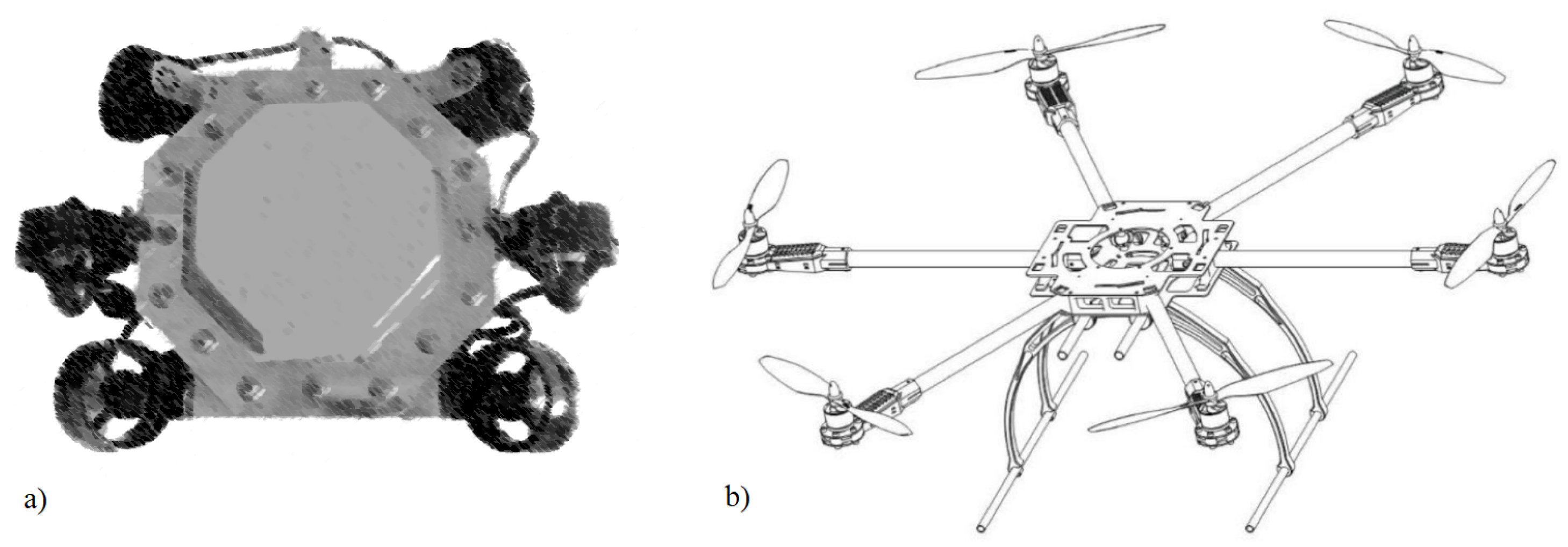
As examples of a k-out-of-n model application, we consider two real-world systems. One of them is described in [24], where an automated system for the remote monitoring of underwater sections of a gas pipeline was considered. One of the essential parts of the system is an unmanned underwater vehicle (UUV) (see Figure 1a), which carries out a visual inspection of underwater areas with the fixation of video materials. It is fitted with various equipment for monitoring, collecting, and transmitting information about the state of the object. Six engines located on different sides of the apparatus allow it to descend, float, and move along the pipe. UUV fails when three engines fail. In addition, the failure of each engine increases the load on the remaining ones, which leads to a decrease in their remaining lifetime. Thus, this system can be represented as a 3-out-of-6 model.

Figure 1. Systems described with k-out-of-n models ((a) unmanned underwater vehicle, (b) copter).

In papers [11,30], a similar model was used for modeling a tethered high-altitude unmanned telecommunication platform for transmitting information on the “last mile” (see Figure 1b). This system can be used in different versions: for $n=6$ or for $n=8$, etc. Different ways of exploitation and failure are also possible. In our numerical experiments, we will refer to this example by modeling it with a 3-out-of-6 model.

Both examples will be used in numerical experiments to demonstrate the impact of system component failures on the decision to choose a certain PM strategy and its sensitivity to the initial information. Numerical analysis of the model is presented in Section 5.

2. The Problem Set, Notations, and Assumptions

2.1. Notations and Assumptions

We consider a k-out-of-n system that consists of n components in parallel and fails if at least k of them fail. It is assumed that the failure of any component leads to an increase in the load on others and, consequently, to a decrease in their residual lifetimes. To increase the reliability of the system, it is supposed that PM based on the observation of the state of the system is possible. We denote by $\mathcal{L}=\{1,2,\dots ,k\}$ the set of possible PM strategies, including running to the system failure for $l=k$. The l-th strategy $(l<k)$ means that the PM begins when l components fail. The strategy $l=k$ means that the PM is not used, and the best solution is to wait for the system to fail and start repairing it jointly with maintenance.

In this paper, we will use the following notations and main assumptions:

• $\mathbf{P}\{·\},\mathbf{E}[·],\mathbf{Var}[·]$—symbols of probability, expectation, and variation;
• $A_i:(i=1,2,\dots )$ is the series of component’s lifetimes, which are assumed to be independent identically distributed random variables;
• $A\left(t\right)=\mathbf{P}\{A_i\le t\}$ is their common cumulative distribution function (cdf) with their probability density function (pdf) $a\left(t\right)=A^{\prime }\left(t\right)$ and expectation

  $$a=\mathbf{E}\left[A_i\right]={\int }_0^{\infty }(1-A_i\left(t\right))dt;$$

  (1)
• The times $B_i^{\left(l\right)}(i=1,2,\dots ),(l\in \mathcal{L})$ of PM and the system repair for $l=k$ are supposed to be independent identically distributed random variables;
• $B_l\left(t\right)=\mathbf{P}\{B_i^{\left(l\right)}\le t\}$ are their cdf with mean values;

  $$b_l=\mathbf{E}\left[B_i^{\left(l\right)}\right]={\int }_0^{\infty }(1-B_l\left(t\right))dt;$$

  (2)
• It is assumed that the mean PM times $b_l(l<k)$ are less than the mean repair time $b_k,b_l\le b_k$, and may or may not depend on the type of maintenance;
• j is the system state, where j means the number of failed components;
• $E=\{j=\{0,1,\dots ,k\left\}\right\}$ is the set of the system states;
• After failure of the l-th component $(l<k)$, the load on all others increases, which leads to a decrease in their residual lifetimes. It is modeled by compression of the residual components lifetime by some weight coefficient $w_i(0\le w_i\le 1)$;
• In the initial time epoch, the system is absolutely reliable, i.e., all its components are in the UP states and the initial system state is $j=0$.
• After any system repair and its PM completion, the system became “as a new one”, i.e., returns to the zero state.

2.2. The Problem Statement

The problem of comparing the PM strategies with respect to the availability of a system with independent failures was considered in paper [24]. This paper continues this study for a model where after the failure of any system component, the load on the other ones increase, resulting in a decrease in the residual lifetime, aiming to maximize the availability factor $K_{\mathrm{av}.,l}$ (other quality criteria are also applicable, such as the productivity of the system and/or system service cost under different maintenance strategies (see [25]))

$$K_{\mathrm{av}.,l}=\underset{t\to \infty }{lim}\frac{1}{t}\left\{\mathrm{the}\mathrm{system}\mathrm{working}\mathrm{time}\mathrm{during}\mathrm{time}t\mathrm{under}\mathrm{strategy}l\right\},$$

(3)

the formal definition of which is represented in (14). To achieve this goal, we define a random process $J=\left\{J\right(t):t\ge 0\}$ with the set of space E by the relation

$$J\left(t\right)=j,\mathrm{if}\mathrm{at}\mathrm{time}t\mathrm{the}\mathrm{system}\mathrm{is}\mathrm{in}\mathrm{the}\mathrm{state}j\in E.$$

(4)

Using this process, we study the main reliability characteristics of a k-out-of-n system under the conditions when the failure of one of its components leads to an increase in the load on the others and, therefore, to a decrease in their residual lifetimes. These are:

• $Y_l,(l\in \mathcal{L})$—system working time during its regeneration cycle (see formal definition in Formula (13)).
• $R_k\left(t\right)$—system reliability function, and $M_k$—mean time until the system fails (after the failure of k components).

  $$R_k\left(t\right)=\mathbf{P}\{Y_k>t\},M_k=\underset{0}{\overset{\infty }{\int }}{R}_k\left(t\right)dt.$$

  (5)
• $F_l\left(t\right)$—cdf of PM start times for different strategies $(l\in \mathcal{L})$, and $M_l$—their expectations

  $$F_l\left(t\right)=\mathbf{P}\{Y_l\le t\},M_l=\underset{0}{\overset{\infty }{\int }}(1-F_l\left(t\right))dt.$$

  (6)
• The system availability $K_{\mathrm{av}.,l}$, $l\in \mathcal{L}$ given by (3) for different PM strategies.
• An indicator of strategy preference criterion, which will be introduced later in the next section.

Moreover, since the initial information about the system component’s lifetime is usually very limited (it is most often possible to obtain only an estimate of the first and second moments of the distribution), we concentrated on studying the sensitivity of any decision about PM strategy choice to the shape of their distributions.

3. Process J and the Main Result

3.1. Process J

For the stated problem solution, consider process J, defined by expression (4) as more detailed. First of all, we note that, by virtue of our assumptions, for any PM strategy $l\in \mathcal{L}$, including running to the system failure for $l=k$, process J is the regenerative one, whose regenerative epochs $S_i^{\left(l\right)}$ are the maintenance or repair completion times. For any regenerative process, the following ergodic theorem holds.

Theorem 1.

For any admissible strategy $l\in \mathcal{L}$ of a controllable (in regeneration epochs) regenerative process $J=\left\{J\right(t),t\ge 0\}$ with a finite expected regeneration period $\mathbf{E}\left[T_i^{\left(l\right)}\right]<\infty$ (where $T_i^{\left(l\right)}=S_i^{\left(l\right)}-S_{i-1}^{\left(l\right)}$) and any integrable function g, defined on the process set of states E, the following limit property holds

$$\underset{t\to \infty }{lim}\frac{1}{t}\underset{0}{\overset{t}{\int }}g\left(J\left(u\right)\right)du=\frac{1}{{\mathbf{E}}_0\left[T_1^{\left(l\right)}\right]}{\mathbf{E}}_0\left[\underset{0}{\overset{T_1^{\left(l\right)}}{\int }}g\left(J\left(u\right)\right)du\right],$$

(7)

where ${\mathbf{E}}_0$ means the expectation given initial state equals zero $i=0$.

Proof. 

For regeneration epochs $S_i^{\left(l\right)}$ of process J, its renewal process will be denoted by

$$N^{\left(l\right)}\left(t\right)=\sum _{i\ge 0}{1}_{\{S_i^{\left(l\right)}\le t\}}$$

(8)

and the left part of equality (7) is represented as

$$\begin{array}{ccc}& & \underset{t\to \infty }{lim}\frac{1}{t}\underset{0}{\overset{t}{\int }}g\left(J\left(u\right)\right)du=\hfill \\ & =& \underset{t\to \infty }{lim}\frac{N^{\left(l\right)}\left(t\right)}{t}\frac{1}{N^{\left(l\right)}\left(t\right)}\sum _{1\le i\le N^{\left(l\right)}\left(t\right)}\left[\underset{S_{i-1}^{\left(l\right)}}{\overset{S_i^{\left(l\right)}}{\int }}g\left(J\left(u\right)\right)du\right]+\frac{1}{t}\underset{S_{N^{\left(l\right)}\left(t\right)}^{\left(l\right)}}{\overset{t}{\int }}g\left(J\left(u\right)\right)du.\hfill \end{array}$$

(9)

Given that, following our assumptions, the last term in this equality tends to zero, according to the limit theorem for the renewal process

$$\underset{t\to \infty }{lim}\frac{N^{\left(l\right)}\left(t\right)}{t}=\frac{1}{{\mathbf{E}}_0\left[T_1^{\left(l\right)}\right]},$$

(10)

and the law of large numbers for independent identically distributed random variables

$$Y_i^{\left(l\right)}=\underset{S_{i-1}^{\left(l\right)}}{\overset{S_i^{\left(l\right)}}{\int }}g\left(J\left(u\right)\right)du$$

(11)

used under the sign of sum as follows

$$\underset{t\to \infty }{lim}\frac{1}{N^{\left(l\right)}\left(t\right)}\sum _{1\le i\le N^{\left(l\right)}\left(t\right)}\left[\underset{S_{i-1}^{\left(l\right)}}{\overset{S_i^{\left(l\right)}}{\int }}g\left(J\left(u\right)\right)du\right]={\mathbf{E}}_0\left[\underset{0}{\overset{T_1^{\left(l\right)}}{\int }}g\left(J\left(u\right)\right)du\right]$$

(12)

that ends the proof.   □

3.2. The Strategy Comparison

The theorem shows that we need to study the behavior of a process only in a separate regeneration period $T_i^{\left(l\right)}=S_i^{\left(l\right)}-S_{i-1}^{\left(l\right)}$ (say the first one $T_1^{\left(l\right)}=S_1^{\left(l\right)}$). Thus, considering function g as an indicator function of the state $l,g\left(j\right)=1_l\left(j\right)$, the integral $Y_i^{\left(l\right)}$ takes the value (since they are independent identically distributed random variables, we omit the lower index and place the upper index below)

$$Y_i^{\left(l\right)}\equiv Y_1^{\left(l\right)}=\underset{0}{\overset{S_1^{\left(l\right)}}{\int }}{1}_l\left(J\left(u\right)\right)du=inf\{t:J\left(t\right)=l,t\le S_1^{\left(l\right)}\}\equiv Y_l,$$

(13)

which equals the time of the l-th type maintenance beginning (the time for the l-th system component failure, the system lifetime for $l=k$) in a separate regeneration period. We denote its mean value by $M_l=\mathbf{E}\left[Y_l\right].$ Then the system availability for different PM strategies $l\in \mathcal{L}$ takes the form

$$K_{\mathrm{av}.,l}=\frac{M_l}{\mathbf{E}\left[T_l\right]}.$$

(14)

Hence, by virtue of the properties of regenerative processes, to calculate the availability $K_{\mathrm{av}.,l}$, we only need the mean value $\mathbf{E}\left[T_l\right]$ of the regeneration period $T_l$ and the mean value $M_l=\mathbf{E}\left[Y_l\right]$ of the working time $Y_l$ in it. Since the regeneration period for any PM strategy $l\in \mathcal{L}$ is $T_l=Y_l+B_l,$ and it is assumed that the mean PM and repair times $b_l=\mathbf{E}\left[B_l\right]$ are known to a Decision Maker (DM), for the problem solution, it suffices to calculate the expectations $M_l=\mathbf{E}\left[Y_l\right]$. Thus, from Theorem 1, it follows

Theorem 2.

The l-th strategy is preferable to the j-th one ($l\succcurlyeq j$) iff

$$\frac{b_l}{b_j}<\frac{M_l}{M_j}.$$

(15)

Proof. 

The comparison of the different PM strategies with respect to maximizing the system availability given by (14) leads to a comparison of the expressions

$$K_{\mathrm{av}.,l}=\frac{M_l}{M_l+b_l}$$

(16)

and because the l-th preventive maintenance strategy is preferable to the j-th one, if $K_{\mathrm{av}.,l}>K_{\mathrm{av}.,j}$ from the inequality

$$\frac{M_l}{M_l+b_l}>\frac{M_j}{M_j+b_j}$$

(17)

it follows that the l-th strategy is preferable to the j-th one ($l\succcurlyeq j$) if and only if $M_l{b}_j>M_j{b}_l$, which in terms of dimensionless indexes, can be rewritten as (15), that ends the proof.    □

4. Distribution of PM Start and System Failure Times

4.1. Distribution of Order Statistics

It is evident that the l-th PM start time (including system failure for $l=k$) is the time of the l-th component failure, in which the l-th order statistics will be denoted as $X_i=A_{\left(i\right)}$ from n iid rvs $A_i(i=1,2,\dots ,n)$ with given cdf $A\left(t\right)$. Their distributions are very well studied (see, for example, [31]). In particular, it has been shown in this book that the joint pdf $f_l(x_1,\dots x_l)$ of the l first-order statistics

$$X_1\le X_2\le \cdots \le X_l$$

(18)

from a sample of n iid rv $A_1,A_2,\dots ,A_n$ with cdf $A\left(x\right)$ and pdf $a\left(x\right)$ in the domain $0\le x_1\le x_2\le \cdots \le x_l<\infty$ equals

$$f_{\mathbf{l}}(x_1,x_2,\dots ,x_l)=\frac{n!}{(n-l)!}a\left(x_1\right)a\left(x_2\right)\cdots a\left(x_l\right){(1-A\left(x_l\right))}^{n-l}.$$

(19)

Remark 1.

From the other side, the individual l-th order statistics distribution does not depend on the positions of all its previous and equals (see also [31])

$$f_l\left(x\right)=\frac{n!}{(n-l)!(l-1)!}A{\left(x\right)}^{l-1}(1-A_l){)}^{n-l}a\left(x\right).$$

(20)

Therefore, it can be calculated by integrating the joint pdf $f_{\mathbf{l}}(x_1,\dots x_l)$ over all possible $(l-1)!$ permutations of variables $x_i$,

$$\begin{array}{ccc}\hfill f_l\left(x\right)& =& \frac{1}{(l-1)!}\underset{0\le x_i\le x(i=\overline{1,l-1})}{\int \cdots \int }{f}_{\mathbf{l}}(x_1,\dots x_{l-1},x)d{x}_1\dots d{x}_{l-1}=\hfill \\ & =& \frac{n!}{(n-l)!(l-1)!}\underset{0\le x_i\le x(i=\overline{1,l-1})}{\int \cdots \int }a\left(x_1\right)a\left(x_2\right)\cdots a\left(x\right){(1-A\left(x\right))}^{n-l}=\hfill \\ & =& \frac{n!}{(n-l)!(l-1)!}A{\left(x\right)}^{l-1}(1-A_l){)}^{n-l}a\left(x\right).\hfill \end{array}$$

(21)

However, if after the failure of one of the components, the load on all others changes, their residual lifetimes also change. Thus, in the next subsection, we consider the transformation of order statistics due to load changes. It will be used further to calculate the pdf of the order statistics in the case of their transformations.

4.2. Transformation of Order Statistics

For the stated problem’s solution, it is necessary to transform order statistics and calculate their distributions in accordance with the accepted rule for a component failure to influence the load on the surviving components. In accordance with this rule, after failure of the i-th component, the residual lifetimes of all survived components are reduced by multiplying by some weight coefficient $w_i$.

Keep in mind that $Y_l(l=\overline{1,k})$ denotes the time to the l-th component failure (time to the l-th PM strategy beginning) or the system failure time for $l=k$ in conditions of load changing after any of its components fail. We represent it in terms of its initial lifetime (order statistics $X_i$). It should be noted that for the considered system with dependent failure times, each subsequent l-th failure leads to compression of the intervals between successive j-th $(j>l)$ and l-th failure times by $w_1\dots w_l$ times, $Y_j=Y_l+w_1\dots w_l(X_j-X_l).$ Thus, for the times $Y_l$ of the l-th state destination, the following generating recursive representation in terms of initial order statistics holds,

$$Y_{l+1}=Y_l+w_1\cdots w_l(X_{l+1}-X_l).$$

(22)

Based on this recursive relation, we prove the following explicit representation of the rvs $Y_l$ in terms of order statistics.

Lemma 1.

The time $Y_l$ to the l-th PM start (system failure time for $l=k$) is a linear function of order statistics:

$$\begin{array}{ccc}\hfill Y_1& =& X_1\mathrm{and}\mathrm{for}l=\overline{2,k}\hfill \\ \hfill Y_l& =& (1-w_1)X_1+w_1(1-w_2)X_2+\cdots +w_1\cdots w_{l-2}(1-w_{l-1})X_{l-1}+\hfill \\ & +& w_1\cdots w_{l-1}{X}_l.\hfill \end{array}$$

(23)

Proof. 

To prove the lemma, we use mathematical induction. The initial component failure times coincide with the first-order statistics $A_{\left(1\right)}=X_1$. After the first failure at time $X_1$, all other expected failure times equal

$$Y_j=X_1+w_1(X_j-X_1)=(1-w_1)X_1+w_1{X}_j$$

(24)

and, therefore,

$$Y_2=X_1+w_1(X_2-X_1)=(1-w_1)X_1+w_1{X}_2,$$

(25)

which coincides with (23) for $l=2$ and gives the possibility to begin the induction procedure. Thus, we suppose that equality (23) holds for any $l<k$, and check it for $l+1$. Using recursive Formula (22), representing the value $Y_{l+1}$ in terms of $Y_l$, one can find

$$\begin{array}{ccc}\hfill Y_{l+1}& =& Y_l+w_1\cdots w_l(X_{l+1}-X_l)=\hfill \\ & =& (1-w_1)X_1+w_1\cdots w_{l-2}(1-w_{l-1})X_{l-1}+w_1\cdots w_{l-1}{X}_l+\hfill \\ & +& w_1\cdots w_l(X_{l+1}-X_l)=\hfill \\ & =& (1-w_1)X_1+w_1\cdots w_{l-2}(1-w_{l-1})X_{l-1}+w_1\cdots w_{l-1}{X}_l+\hfill \\ & +& w_1\cdots w_l{X}_{l+1}-w_1\cdots w_l{X}_l=\hfill \\ & =& (1-w_1)X_1+w_1\cdots w_{l-1}(1-w_l)X_l+w_1\cdots w_l{X}_{l+1,}\hfill \end{array}$$

(26)

that ends the proof.    □

4.3. Distribution of the Random Variables $Y_l$

Now we proceed to the calculation of the cdf $F_{Y_l}\left(t\right)$ of the time $Y_l$ to the l-th component failure, taking into account the redistribution of the load on the components. Here we perform this using expression (23) for the time to the l-th component failure in terms of order statistics $X_i$ and Formula (19) for the joint distribution of the first l-order statistics. To simplify the representation of this cdf, let us introduce the following notations.

$$\begin{array}{ccc}\hfill z_0& =& t,\mathrm{and}\mathrm{for}(i=\overline{1,l-1});\hfill \\ \hfill z_i& =& z_i(t;x_1,\dots ,x_i)=\hfill \\ & =& \frac{t-(1-w_1)x_1-w_1(1-w_2)x_2-\cdots -w_1\cdots w_{i-1}{x}_{i-1}}{w_1\cdots w_i}.\hfill \end{array}$$

(27)

With these notations, the following theorem holds.

Theorem 3.

The distribution of the l-th component failure (time to the l-th PM beginning) for $t\ge 0$ is

$$\begin{array}{ccc}\hfill & & F_{Y_l}\left(t\right)=\mathbf{P}\{Y_l\le t\}=\hfill \\ & =& \frac{n!}{(n-k)!}\underset{0}{\overset{z_0}{\int }}a\left(x_1\right)d{x}_1\underset{x_1}{\overset{z_1}{\int }}a\left(x_2\right)d{x}_2\cdots \underset{x_{l-1}}{\overset{z_{l-1}}{\int }}a\left(x_l\right){(1-A\left(x_l\right))}^{n-l}d{x}_l.\hfill \end{array}$$

(28)

Proof. 

Lemma 1 states that the time $Y_l$ of the l-th component failure is a linear function of the first l-order statistics (as shown by Formula (23)). Consequently, given the pdf $f_l(x_1,\dots ,x_l)$ of the l-th order statistics, we can derive the cdf $F_{Y_l}\left(t\right)$ of rv $Y_l$

$$\begin{array}{ccc}\hfill F_{Y_l}\left(t\right)& =& \mathbf{P}\{Y_l\le t\}=\hfill \\ & =& \mathbf{P}\{(1-w_1)X_1+w_1(1-w_2)X_2+\cdots +\hfill \\ & +& w_1\cdots w_{l-2}(1-w_{l-1})X_{l-1}+w_1\cdots w_{l-1}{X}_l\le t\}=\hfill \\ & =& \underset{D(t;x_1,\dots ,x_l)}{\int \cdots \int }{f}_l(x_1,x_2,\dots ,x_l)d{x}_1\dots d{x}_l,\hfill \end{array}$$

(29)

where the integration domain $D(t:x_1,\dots ,x_l)$ is the intersection of two subsets of l-dimensional space, $D(t;x_1,\dots ,x_l)=D_{+}^{\left(l\right)}\cap D_w^{\left(l\right)}\left(t\right)$, where $D_{+}^{\left(l\right)}$ is the first quadrant of the l-dimensional space: $D_{+}^{\left(l\right)}=\{0\le x_1\le \cdots \le x_l\}$ and the hyperspace $D_w^{\left(l\right)}\left(t\right)$ is

$$\begin{array}{ccc}\hfill D_w^{\left(l\right)}\left(t\right)& =& \{(1-w_1)x_1+w_1(1-w_2)x_2+\cdots +w_1\cdots w_{l-2}(1-w_{l-1})x_{l-1}+\hfill \\ & +& w_1\cdots w_{l-1}{x}_l\le t\}.\hfill \end{array}$$

(30)

The multidimensional integral (29) can be transformed into an iterated one. Given $0\le x_1\le x_2\le \cdots \le x_l$, the integration domain can be represented according to the following procedure. From inequality (30) for variable $x_l$, it follows that

$$x_l\le \frac{t-w_1{x}_1-w_1(1-w_2)x_2-\cdots -w_1\cdots w_{i-1}{x}_{l-1}}{w_1\cdots w_{l-1}}=z_{l-1}(t;x_1\dots x_{l-1}).$$

(31)

Further, also given $x_{l-1}\le x_l$ from inequality (31), it follows that

$$x_{l-1}\le x_l\le \frac{t-w_1{x}_1-w_1(1-w_2)x_2-\cdots -w_1\cdots w_{l-1}{x}_{l-1}}{w_1\cdots w_{l-1}}.$$

(32)

From inequality (32), using algebraic manipulations, one can find

$$\begin{array}{ccc}\hfill x_{l-1}& \le & \frac{t-w_1{x}_1-w_1(1-w_2)x_2-\cdots -w_1\cdots w_{l-2}{x}_{l-2}}{w_1\cdots w_{l-2}}=\hfill \\ & =& z_{l-2}(t;x_1\dots x_{l-2}).\hfill \end{array}$$

(33)

In a similar way, we obtain the following inequality for the variable $x_2$

$$\begin{array}{ccc}\hfill t& \ge & (1-w_1)x_1+w_1(1-w_2)x_2+w_1{w}_2{x}_3\ge \hfill \\ & \ge & (1-w_1)x_1+w_1(1-w_2)x_2+w_1{w}_2{x}_2=(1-w_1)x_1+w_1{x}_2,\hfill \end{array}$$

(34)

from which it follows that

$$x_2\le \frac{t-(1-c_1)x_1}{c_1}=z_2(t:x_1).$$

(35)

Further, at last,

$$t\ge (1-w_1)x_1+w_1{x}_1=x_1.$$

(36)

Consequently, $0\le x_1\le t$. Therefore, the integration domain $D(t:x_1,\dots ,x_l)$ in terms of notations (27) can be transformed as

$$D(t:x_1,\dots ,x_l)=\{x_{i-1}\le x_i\le z_i(t;x_1,\dots x_{i-1})(i=\overline{1,l-1})\}.$$

(37)

Thus, using Formula (19) for pdf $f_l(x_1,\dots ,x_l)$ of the first l-order statistics and the integration domain (37), integral (29) for $t\ge 0$ can be written as

$$F_{Y_l}\left(t\right)=\frac{n!}{(n-l)!}\underset{0}{\overset{t}{\int }}a\left(x_1\right)d{x}_1\underset{x_1}{\overset{z_1}{\int }}a\left(x_2\right)d{x}_2\cdots \underset{x_{l-1}}{\overset{z_{l-1}}{\int }}a\left(x_l\right){(1-A\left(x_l\right))}^{n-l}d{x}_l,$$

which coincides with (28) and ends the proof.    □

Based on Theorem 3, the main system reliability characteristics can be obtained, such as:

(i)

its reliability function $R\left(t\right)=1-F_{Y_k}\left(t\right)$;

(ii)

its mean lifetime $\mathbf{E}\left[Y_k\right]={\int }_0^{\infty }R\left(t\right)dt$;

(iii)

availability factor $K_{\mathrm{av}.,l}$ for different PM strategies.

4.4. An Example: Exponential Distribution of Components Lifetimes

In a special case, when the systems’ components lifetimes $A_i(i=\overline{1,n})$ follow an exponential distribution with a parameter $\alpha$ ($Exp(\alpha$)), the integral (28) can be calculated analytically. For this case, we introduce a different approach to the system’s lifetime distribution, which is derived from the memoryless property of an exponential distribution. Let $T_i$ be the time interval between the $i-1$-th and i-th component’s failures, $i=\overline{1,l-1}$ ($T_0=0$). Then, by virtue of the memoryless property of the exponential distribution, the time to the k-th failure $Y_k$ is the sum

$$Y_l=T_1+T_2+\cdots +T_l,$$

(38)

of l independent exponentially distributed rvs $T_i$ with mean values

$$\mathbf{E}\left[T_1\right]=\frac{1}{n\alpha },\mathbf{E}\left[T_i\right]=\frac{w_1{w}_2\cdots w_{i-1}}{(n-i+1)\alpha }=\frac{{\overline{w}}_i}{(n-i+1)\alpha },(i=\overline{2,l}).$$

(39)

This means that the parameters of their distribution are:

$${\lambda }_1=n\alpha ,{\lambda }_i=\frac{(n-i+1)\alpha }{w_1{w}_2\cdots w_{i-1}}=\frac{(n-i+1)\alpha }{{\overline{w}}_i},(i=\overline{2,l}),$$

(40)

where, for purposes of simplicity, we introduce the notation:

$${\overline{w}}_i=\left\{\begin{array}{cc}1,\hfill & i=1,\hfill \\ w_1\cdots w_{i-1},\hfill & i=\overline{2,l}.\hfill \end{array}\right.$$

(41)

The general case can be studied with the help of the moment-generating function (mgf) of the system lifetime, which, in this case, has the following form:

$${\varphi }_k\left(s\right)=\mathbf{E}\left[e^{-s{Y}_k}\right]=\prod _{1\le i\le k}\mathbf{E}\left[e^{-s{T}_i}\right]=\prod _{1\le i\le k}\frac{{\lambda }_i}{s+{\lambda }_i}.$$

(42)

However, the cdf calculation from this expression is not a simple problem, and we limit ourselves to the simplest example of a k-out-of-n model with $k=2$ and first calculate the cdf of $Y_2$ directly. In this case, we assume $w_1=w$. Hence, following (19), the joint distribution of rv $X_1,X_2$ is

$$f_2(x_1,x_2)=\frac{n!}{(n-2)!}a\left(x_1\right)a\left(x_2\right){(1-A\left(x_2\right))}^{n-2}=\frac{n!}{(n-2)!}{\alpha }^2{e}^{-\alpha x_1}{e}^{-(n-1)\alpha x_2}.$$

(43)

Calculate cdf $F_{Y_2}\left(t\right)$ of the rv $Y_2=(1-w)X_1+w{X}_2$,

$$\begin{array}{ccc}\hfill F_{Y_2}\left(t\right)& =& \mathbf{P}\{(1-w)X_1+w{X}_2<t\}=\mathbf{P}\left\{X_2<\frac{t-(1-w)X_1}{w}\right\}=\hfill \\ & =& n(n-1){\alpha }^2\underset{0}{\overset{t}{\int }}{e}^{-\alpha x_1}d{x}_1\underset{x_1}{\overset{\frac{t-(1-w)x_1}{w}}{\int }}{e}^{-(n-1)\alpha x_2}d{x}_2=\hfill \\ & =& 1+\frac{n-1}{nw-(n-1)}{e}^{-n\alpha t}-\frac{nw}{nw-(n-1)}{e}^{-\frac{(n-1)\alpha }{w}t},\hfill \end{array}$$

(44)

and, therefore, its pdf for $t\ge 0$ is

$$f_{Y_2}\left(t\right)=\frac{n(n-1)\alpha }{nw-(n-1)}\left(e^{-\frac{(n-1)\alpha }{w}t}-e^{-n\alpha t}\right).$$

(45)

It should be noted that this result is valid for $w\ne (n-1)/n$, in which case the distribution is a mixture of exponential distributions. The point $w=(n-1)/n$ is a singular point for which cdf of the rv $Y_2$ follows an Erlang distribution,

$$F_{Y_2}\left(t\right)=1-e^{-n\alpha t}-n\alpha t{e}^{-n\alpha t},t>0,$$

(46)

with pdf

$$f_{Y_2}\left(t\right)=n^2{\lambda }^{2}t{e}^{-n\lambda t},t>0.$$

(47)

Remark 2.

The singularity in the calculation of the cdf of the system lifetime arises because, for some special values of coefficient $w_i$ (here for $w=(n-1)/n$), the moment-generating function of the system’s lifetime has multiple roots that lead to changing the shape of the distribution.

Using another approach, the mgf of the system’s lifetime can be written as follows:

$${\varphi }_2\left(s\right)=\frac{n(n-1){\alpha }^2}{s^2+(2n-1)\alpha s+n(n-1){\alpha }^2}.$$

(48)

By decomposing this expression, one finds

$${\varphi }_2\left(s\right)={\displaystyle \frac{(n-1)n\alpha }{s+n\alpha }}-{\displaystyle \frac{(n-1)n\alpha }{s+(n-1)\alpha }},$$

(49)

the inverse function, then, is calculated as

$$f_2\left(t\right)=n(n-1)\alpha \left(e^{-(n-1)\alpha t}-e^{-n\alpha t}\right),$$

(50)

which coincides with the result obtained in (45) for $w=1$.

Apparently, analytic results are not to be expected in the general case. However, one can hope for numerical calculations of examples with different distributions of the random variable $A_i$. Thus, based on Theorem 2, we propose a recursive procedure for calculating distributions $F_l\left(t\right)$ of random variable $Y_l$($l=\overline{1,k}$) and their moments. Based on this calculation, the PM strategies comparison as advice to DM will be done. Below an Algorithm for the problem solution is proposed.

5. An Algorithm for the PM Strategies Comparison and Numerical Experiments

5.1. Algorithm

On the basis of the results of Section 4, the general procedure for the problem solution can be implemented with the following algorithm (Algorithm 1).

Algorithm 1 General algorithm for calculation of the reliability function.

Beginning. Determine: Integers $n,k$, real $b_0,b_l(l=\overline{1,k}))$, $w_l(l=\overline{1,k})$, distribution $A\left(t\right)$ of the system components’ lifetime, its pdf, expectation a and coefficient of variation v.          Step 1. Calculate parameters of cdf $A\left(t\right)$ in terms of its expectation a and coefficient of variation v.          Step 2. Taking into account the joint pdf of the first l order statistics $X_1\le X_2\le \cdots \le X_l$ $$f_l(x_1,x_2,\dots ,x_l)=\frac{n!}{(n-l)!}a\left(x_1\right)a\left(x_2\right)\dots a\left(x_l\right){(1-A\left(x_l\right))}^{n-l},$$ (51)          calculate according to (28) the rv $Y_l$ cdf $$\begin{array}{c}\hfill F_{Y_l}\left(t\right)=\frac{n!}{(n-l)!}\underset{0}{\overset{z_0}{\int }}a\left(x_1\right)d{x}_1\underset{x_1}{\overset{z_1}{\int }}a\left(x_2\right)d{x}_2\cdots \underset{x_{l-1}}{\overset{z_{l-1}}{\int }}a\left(x_l\right){(1-A\left(x_l\right))}^{n-l}d{x}_l,\end{array}$$ (52) where the limits of integration are determined by the relation (27) $$\begin{array}{ccc}\hfill z_0& =& t,\mathrm{and}\mathrm{for}(i=\overline{1,l-1});\hfill \\ \hfill z_i& =& z_i(t;x_1,\dots ,x_i)=\hfill \\ & =& \frac{t-(1-w_1)x_1-w_1(1-w_2)x_2-\cdots -w_1\cdots w_{i-1}{x}_{i-1}}{w_1\cdots w_i}.\hfill \end{array}$$ (53)          Step 3. Calculate the function $R_l\left(t\right)=1-F_{Y_l}\left(t\right)$ and the mean time to the PM strategy beginning (mean time to the l-th component failure) $$M_l=\mathbf{E}\left[Y_l\right]=\underset{0}{\overset{\infty }{\int }}{R}_l\left(t\right)dt,$$ (54)          and the availability factor $$K_{\mathrm{av}.,l}=\frac{M_l}{M_l+b_l}.$$ (55)          Step 4. Compare the PM strategies by the criterion (15) $$\frac{b_l}{b_j}<\frac{M_l}{M_j}$$ (56) and chose the best one.          Stop.

Remark 3.

The algorithm might also be useful for other purposes, such as analysis of the sensitivity of the system reliability function and its characteristics to the shape of the lifetime distribution of the system components.

5.2. Numerical Experiments

Based on the algorithm, we consider some numerical experiments. For the numerical analysis, we use the four most popular distributions of non-negative random variables: (i) exponential ($Exp\left(\lambda \right)$), (ii) Gamma ($\mathsf{\Gamma }(\lambda ,\mathsf{\Theta })$), (iii) Gnedenko–Weibull ($GW(\lambda ,\mathsf{\Theta })$), and (iv) lognormal ($LN(\mu ,\sigma ))$). The corresponding rvs are denoted as $E,\mathsf{\Gamma },GW,LN$. All of these distributions (except for the exponential), for some of their parameters, became the so-called “heavy tailed ones”, which imposes certain restrictions on the computational procedures associated with their use.

The Gamma distribution with parameters $(\lambda >0,\mathsf{\Theta }>0)$ has the pdf and cdf of the form

$$f_{\mathsf{\Gamma }}\left(x\right)=\frac{1}{\mathsf{\Gamma }\left(\mathsf{\Theta }\right){\lambda }^{\mathsf{\Theta }}}{x}^{\mathsf{\Theta }-1}{e}^{-\frac{x}{\lambda }},F_{\mathsf{\Gamma }}\left(x\right)=\frac{1}{\mathsf{\Gamma }\left(\mathsf{\Theta }\right){\lambda }^{\mathsf{\Theta }}}\underset{0}{\overset{x}{\int }}{t}^{\mathsf{\Theta }-1}{e}^{-\frac{t}{\lambda }}dt,$$

where $\mathsf{\Gamma }\left(\mathsf{\Theta }\right)$ is the Gamma function. Its expectation, variance, and coefficient of variation have the form

$$\mathbf{E}\left[\mathsf{\Gamma }\right]=\lambda \mathsf{\Theta },\mathbf{Var}\left[\mathsf{\Gamma }\right]={\lambda }^2\mathsf{\Theta },v_{\mathsf{\Gamma }}=\frac{1}{\sqrt{\mathsf{\Theta }}}.$$

Concerning the $GW$-distribution with parameters $(\lambda >0,\mathsf{\Theta }>0)$, it has the pdf and the cdf of the form

$$f_{GW}\left(x\right)=\frac{\mathsf{\Theta }}{\lambda }{\left(\frac{x}{\lambda }\right)}^{\theta -1}{e}^{-{\left(\frac{x}{\lambda }\right)}^{\mathsf{\Theta }}},F_{GW}\left(t\right)=1-e^{-{\left(\frac{t}{\lambda }\right)}^{\mathsf{\Theta }}},$$

its coefficient of variation v depends only on parameter $\mathsf{\Theta }$

$$v^2+1=\frac{\mathsf{\Gamma }(1+\frac{2}{\mathsf{\Theta }})}{{\mathsf{\Gamma }}^2(1+\frac{1}{\mathsf{\Theta }})}=\frac{\frac{2}{\mathsf{\Theta }}\mathsf{\Gamma }\left(\frac{2}{\mathsf{\Theta }}\right)}{{\frac{1}{\mathsf{\Theta }}}^2{\mathsf{\Gamma }}^2\left(\frac{1}{\mathsf{\Theta }}\right)}=2\mathsf{\Theta }\frac{\mathsf{\Gamma }\left(\frac{2}{\mathsf{\Theta }}\right)}{{\mathsf{\Gamma }}^2\left(\left(\frac{1}{\mathsf{\Theta }}\right)\right)}.$$

For $0<\mathsf{\Theta }\le 1$, for example $\mathsf{\Theta }=\frac{1}{l}$ it holds

$$v^2+1=(l+1)\cdots (2l-1)\to \infty$$

Specifically, for $\mathsf{\Theta }=0.5$, it gives $v=\sqrt{2}$, for $\mathsf{\Theta }=\frac{1}{3}$ it gives $v^2+1=20$. Thus, the $GW$ distribution for $\mathsf{\Theta }<1$ has a heavy tail, which forces us to confine ourselves to studying the behavior of the model, in this case, by the range of values of coefficient of variation $v\le \sqrt{2}$.

For $\mathsf{\Theta }\ge 1$, this distribution is a light-tailed one. In this case, putting $\mathsf{\Theta }=\frac{1}{ϵ}$ note that the behavior of its coefficient of variation depends on the behavior of the function $\frac{\mathsf{\Gamma }\left(2ϵ\right)}{ϵ{\mathsf{\Gamma }}^2\left(ϵ\right)}$ around $ϵ=0$.

For $\mathsf{\Theta }=1$, both of the above distributions turn into an exponential.

For the $LN(\mu ,{\sigma }^2)$ distribution, its pdf and cdf are

$$f_{LN}\left(x\right)=\frac{1}{x\sigma \sqrt{\pi }}exp\left\{-\frac{1}{2}{\left(\frac{lnx-\mu }{\sigma }\right)}^2\right\},F_{LN}\left(x\right)=\frac{1}{2}\left[1+\left(\frac{lnx-\mu }{\sigma \sqrt{2}}\right)\right].$$

Its expectation, variation, and coefficient of variation are

$$\mathbf{E}\left[LN\right]=e^{\mu +\frac{{\sigma }^2}{2}},\mathbf{Var}\left[LN\right]=\left(e^{{\sigma }^2}-1\right)e^{\mu +\frac{{\sigma }^2}{2}},v_{\left[LN\right]}=\sqrt{e^{{\sigma }^2}-1}.$$

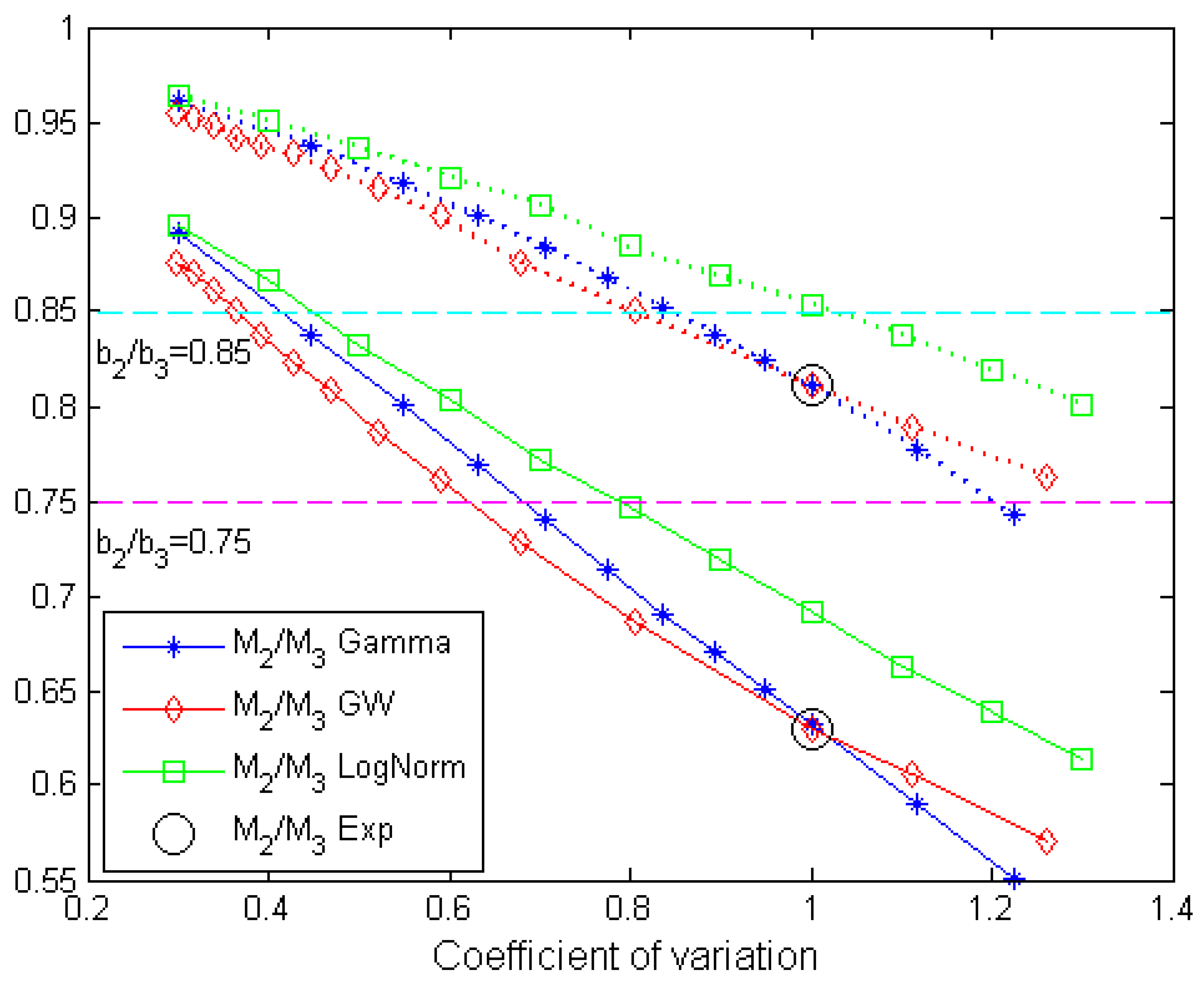
In the numerical experiments below, the parameters of the distributions were taken such that the mean operating time of the system components was equal to 1 (which, accordingly, meant the unit of time measurement), and another parameter provided the coefficient of variation in the domain $0.3\le v\le 1.3$. Figure 2 presents a comparison of “2-strategy” and ”3-strategy” for different system components’ lifetime distributions and coefficients of variation. Solid lines present the calculations for $w_1=w_2=0.9$, and dashed lines demonstrate the results for $w_1=w_2=0.5$. Blue lines show the results for the Gamma distribution of the component’s lifetime, red is for the Gnedenko–Weibul distribution, green is for the lognormal one, and black presents the exponential distribution. For the exponential distribution, the analytical results coincide with the numerical calculations.

Figure 2. Comparison of “2-strategy” and ”3-strategy” for different coefficients of variation.

Let the ratio of PM time after two failures and after three failures be $b_2/b_3=0.75$ and $w_1=w_2=0.9$. For the exponential distribution of the system components’ lifetime, the “3-strategy” of PM should be chosen. If the variation of system components’ lifetime is less than 0.6, the “2-strategy” is preferable to the “3-strategy” for Gamma, GW, and LN distributions. If the variation of the system components’ lifetime is greater than 0.8, the “3-strategy” is preferable to the “2-strategy” for Gamma, GW, and LN distributions. In the interval $[0.6,0.8]$, the choice of strategy depends on the lifetime distribution of system components.

We may conclude that for small values of $w_i$ and variation, the difference between Gamma and GW distributions is insignificant. For the LN distribution, the interval of variation prefers the “2-strategy” over the “3-strategy”.

5.3. An Example: Exponential Distribution

In the case of an exponential distribution based on Formula (42) for the system 2-out-of-6, the following can be written

$${\varphi }_2\left(s\right)=\frac{{\lambda }_1}{s+{\lambda }_1}\frac{{\lambda }_2}{s+{\lambda }_2},$$

where ${\lambda }_1=6\alpha ,{\lambda }_2=\frac{5\alpha }{w}$. Therefore,

$${\varphi }_1^{\prime }\left(s\right)=-\frac{{\lambda }_1{\lambda }_2}{\left[(s+{\lambda }_1)\right](s+{\lambda }_2){]}^2},$$

and

$$M_2=-{\varphi }_1^{\prime }\left(0\right)=\frac{1}{{\lambda }_1}+\frac{1}{{\lambda }_2}=\frac{1}{6\alpha }+\frac{w}{5\alpha }.$$

Analogously, for the 3-out-of-6 system it holds

$${\varphi }_3\left(s\right)=\frac{{\lambda }_1}{s+{\lambda }_1}\frac{{\lambda }_2}{s+{\lambda }_2}\frac{{\lambda }_3}{s+{\lambda }_3},$$

where ${\lambda }_1,{\lambda }_2$ are the same as before, and ${\lambda }_3=\frac{4\alpha }{w^2}$. By calculation of the derivative of mgf ${\varphi }_3\left(s\right)$ in points $s=0$ and taking into account the values of parameters ${\lambda }_i$, one can find

$$M_3=-{\varphi }_3^{\prime }\left(0\right)=\frac{1}{6\alpha }+\frac{w}{5\alpha }+\frac{w^2}{4\alpha }.$$

For the given $\alpha =1$ and $w=0.5$ and $w=0.9$, these values coincide with the point in Figure 2.

6. Conclusions

The paper is devoted to the investigation of different PM strategies for the controllable k-out-of-n system based on its stated observation. It is supposed that after a failure of one of the system components, the load on all the others increases, which leads to a decrease in their residual lifetime. The novelty of the paper lies in the application of order statistics for modeling the residual lifetime of system components and developing a procedure for comparing PM strategies with respect to the availability maximization criterion, which is presented in the form of an algorithm.

A series of numerical experiments were performed for real examples modeled as a 3-out-of-6 system with exponential, Gamma, Gnedenko–Weibull, and Lognormal distributions and different coefficients of variation. The results revealed the sensitivity of the choice of PM strategy to the shape of lifetime’s distribution of the system components and the coefficient of variation. Nevertheless, it is possible to identify intervals for the coefficient of variation, where the choice of the preferable strategy is independent of the type of distribution.

The presented approach can be further expanded, involving more quality criteria, such as the productivity of the system or system service cost under different maintenance strategies, and a multi-criteria evaluation of the PM effectiveness is feasible as well. The calculations have been performed for the example of the 3-out-of-6 system, but the proposed procedure can be used for other systems. This article is theoretical in nature, and we invite persons with specific information to cooperate and further research the proposed direction.

References

- Shepherd, D. k-out-of-n Systems. In Encyclopedia of Statistics in Quality and Reliability; John Wiley & Sons: Hoboken, NJ, USA, 2008; Available online: https://onlinelibrary.wiley.com/doi/pdf/10.1002/9780470061572.eqr342/ (accessed on 18 February 2022).
- Trivedi, K. Probability and Statistics with Reliability, Queuing and Computer Science Applications, 2nd ed.; John Wiley & Sons: Hoboken, NJ, USA, 2016; Available online: https://onlinelibrary.wiley.com/doi/book/10.1002/9781119285441 (accessed on 18 February 2022).
- Chakravarthy, S.; Krishnamoorthy, A.; Ushakumari, P. A (k-out-of-n) reliability system with an unreliable server and Phase type repairs and services: The (N,T) policy. J. Appl. Math. Stoch. Anal. 2001, 14, 361–380. [Google Scholar] [CrossRef]
- Yuge, T.; Maruyama, M.; Yanagi, S. Reliability of a (k-out-of-n) system with common-cause failures using multivariate exponential distribution. Procedia Comput. Sci. 2016, 96, 968–976. [Google Scholar] [CrossRef]
- Zhang, T.; Xie, M.; Horigome, M. Availability and reliability of (k-out-of-(M+N)): Warm standby systems. Reliab. Eng. Syst. Saf. 2006, 91, 381–387. [Google Scholar] [CrossRef]
- Kuo, W.; Zuo, M. Optimal Reliability Modeling: Principles and Applications; John Wiley & Sons: Hoboken, NJ, USA, 2003. [Google Scholar]
- Wang, K.H.; Chen, W.L.; Yang, D.Y. Optimal management of the machine repair problem with working vacation: Newton’s method. Comput. Appl. Math. 2009, 233, 449–458. [Google Scholar] [CrossRef]
- Ke, J.C.; Hsu, Y.L.; Liu, T.H.; Zhang, Z.G. Computational analysis of machine repair problem with unreliable multi-repairmen. Comput. Oper. Res. 2013, 40, 848–855. [Google Scholar] [CrossRef]
- Wang, K.H.; Ke, J.B.; Ke, J.C. Profit analysis of the M/M/R machine repair problem with balking, reneging, and standby switching failures. Comput. Oper. Res. 2007, 34, 835–847. [Google Scholar] [CrossRef]
- Rykov, V.V.; Sukharev, M.G.; Itkin, V.Y. Investigations of k-out-of-n Systems Application Possibilities to Objects of Oil And Gas Industry. J. Mar. Sci. Eng. 2020, 8, 928. [Google Scholar] [CrossRef]
- Vishnevsky, V.M.; Kozyrev, D.V.; Rykov, V.V.; Nguyen, Z.F. Reliability Modeling of an unmanned high-altitude module of a tethered telecommunications platform. Inform. Technol. Comput. Syst. 2020, 4, 26–38. (In Russian) [Google Scholar] [CrossRef]
- Ying, C.; Qichao, M.; Ze, W.; Yingyi, L. Reliability analysis of k-out-of-n system with load-sharing and failure propagation effect. J. Syst. Eng. Electron. 2021, 32, 1221–1231. [Google Scholar] [CrossRef]
- Sharifi, M.; Taghipour, S.; Abhari, A. Inspection interval optimization for a k-out-of-n load sharing system under a hybrid mixed redundancy strategy. Reliab. Eng. Syst. Saf. 2021, 213, 107681. [Google Scholar] [CrossRef]
- Ahmadi, R. Reliability and maintenance modeling for a load-sharing k-out-of-n system subject to hidden failures. Comput. Ind. Eng. 2020, 150, 106894. [Google Scholar] [CrossRef]
- Nezakati, E.; Razmkhah, M. Reliability analysis of a load sharing k-out-of-n: F degradation system with dependent competing failures. Reliab. Eng. Syst. Saf. 2020, 203, 107076. [Google Scholar] [CrossRef]
- Rykov, V.; Ivanova, N.; Kozyrev, D.; Milovanova, T. On Reliability Function of a k-out-of-n System with Decreasing Residual Lifetime of Surviving Components after Their Failures. Mathematics 2022, 10, 4243. [Google Scholar] [CrossRef]
- Gertsbakh, I. Preventive Maintenance Models Based on the Lifetime Distribution. In Reliability Theory with Applications to Preventive Maintenance; Springer: Berlin/Heidelberg, Germany, 2000; pp. 67–106. [Google Scholar]
- Finkelstein, M.; Levitin, G. Preventive maintenance for homogeneous and heterogeneous systems. Appl. Stoch. Model. Bus. Ind. 2019, 35, 908–920. [Google Scholar] [CrossRef]
- Finkelstein, M.; Cha, J.H.; Levitin, G. On a new age-replacement policy for items with observed stochastic degradation. Qual. Reliab. Eng. Int. 2020, 36, 1132–1146. [Google Scholar] [CrossRef]
- Park, M.; Lee, J.; Kim, S. An optimal maintenance policy for k-out-of-n system without monitoring component. Qual. Technol. Qual. Manag. 2019, 16, 140–153. [Google Scholar] [CrossRef]
- Endharth, A.J.; Yun, W.Y.; Yamomoto, H. Preventive maintenance policy for linear-consequtive -k-out-of-n: F system. J. Oper. Res. Soc. Jpn. 2016, 59, 334–346. [Google Scholar]
- Hamdan, K.; Tavangar, M.; Asadi, M. Optimal preventive maintenance for repairable weighted k-out-of-n systems. Reliab. Eng. Syst. Safe 2021, 205, 107267. [Google Scholar] [CrossRef]
- Rezaei, E.; Jafary, B.; Fiondella, L. Optimal maintenance policies for linear consecutive k-out-of-n: F systems susceptible to dependent failures. Comput. Ind. Eng. 2022, 173, 108657. [Google Scholar] [CrossRef]
- Rykov, V.; Kochueva, O.; Farkhadov, M. Preventive Maintenance of a k-out-of-n System with Applications in Subsea Pipeline Monitoring. J. Mar. Sci. Eng. 2021, 9, 85. [Google Scholar] [CrossRef]
- Rykov, V.; Kochueva, O.; Rykov, Y. Preventive Maintenance of k-out-of-n System with Respect to Cost-Type Criterion. Mathematics 2021, 9, 2798. [Google Scholar] [CrossRef]
- Kala, Z. Quantification of Model Uncertainty Based on Variance and Entropy of Bernoulli Distribution. Mathematics 2022, 10, 3980. [Google Scholar] [CrossRef]
- Kala, Z. New Importance Measures Based on Failure Probability in Global Sensitivity Analysis of Reliability. Mathematics 2021, 9, 2425. [Google Scholar] [CrossRef]
- Rykov, V. On Reliability of Renewable Systems. In Reliability Engineering. Theory and Applications; Vonta, I., Ram, M., Eds.; CRC Press: Boca Raton, FL, USA, 2018; pp. 173–196. [Google Scholar]
- Rykov, V.; Kozyrev, D.; Filimonov, A.; Ivanova, N. On reliability function of a k-out-of-n system with general repair time distribution. Probab. Eng. Inf. Sci. 2020, 5, 1–18. [Google Scholar] [CrossRef]
- Vishnevsky, V.; Efrosinin, D.; Krishnamoorthy, A. Principles of Construction of Mobile and Stationary Tethered High-Altitude Unmanned Telecommunication Platforms of Long-Term Operation. In Communications in Computer and Information Science; Springer: Cham, Switzerland, 2018; Volume 919. [Google Scholar] [CrossRef]
- David, H.; Nagaraja, H. Order Statistics, 3rd ed.; John Wiley & Sons: New York, NY, USA, 2003. [Google Scholar]
Disclaimer/Publisher’s Note: The statements, opinions and data contained in all publications are solely those of the individual author(s) and contributor(s) and not of MDPI and/or the editor(s). MDPI and/or the editor(s) disclaim responsibility for any injury to people or property resulting from any ideas, methods, instructions or products referred to in the content. |
© 2023 by the authors. Licensee MDPI, Basel, Switzerland. This article is an open access article distributed under the terms and conditions of the Creative Commons Attribution (CC BY) license (https://creativecommons.org/licenses/by/4.0/).