Quantification of Model Uncertainty Based on Variance and Entropy of Bernoulli Distribution

Abstract

This article studies the role of model uncertainties in sensitivity and probability analysis of reliability. The measure of reliability is failure probability. The failure probability is analysed using the Bernoulli distribution with binary outcomes of success (0) and failure (1). Deeper connections between Shannon entropy and variance are explored. Model uncertainties increase the heterogeneity in the data 0 and 1. The article proposes a new methodology for quantifying model uncertainties based on the equality of variance and entropy. This methodology is briefly called “variance = entropy”. It is useful for stochastic computational models without additional information. The “variance = entropy” rule estimates the “safe” failure probability with the added effect of model uncertainties without adding random variables to the computational model. Case studies are presented with seven variants of model uncertainties that can increase the variance to the entropy value. Although model uncertainties are justified in the assessment of reliability, they can distort the results of the global sensitivity analysis of the basic input variables. The solution to this problem is a global sensitivity analysis of failure probability without added model uncertainties. This paper shows that Shannon entropy is a good sensitivity measure that is useful for quantifying model uncertainties.

1. Introduction

Structural reliability is a measure of the ability of a structure to function without failure when put into operation [1]. A limit state function indicates success or failure states [2]. A structure is considered reliable if the probability of failure P_f is very small.

In the probability theory, the failure frequency can be studied using the Bernoulli distribution, where P_f is the mean value and P_f(1 − P_f) is the variance. Whereas P_f is a an important variable for assessing reliability, variance P_f(1 − P_f) is useful for the global sensitivity analysis of reliability.

Reliability-oriented sensitivity analysis (ROSA) based on the Sobol–Hoeffding decomposition of P_f(1 − P_f) was first introduced in [3,4]. Since then, ROSAs have been applied in studies of the structural reliability of steel [5,6], concrete [7] and composite [8] beams. The concept [3,4] builds on Sobol [9,10], but with its focus on P_f, it surpasses classical methods examining the correlation [11,12], variance [13,14] or distribution [15,16] of model output without a clear relationship to structural reliability.

A generalisation of all types of global sensitivity indices was presented by Fort using contrast functions [17]. It can be noted that ROSA also includes quantile-oriented sensitivity indices, which are useful in load-carrying capacity analysis based on quantiles as design values of the limit states [18,19,20,21,22]. A comparison of selected ROSA types in applications for limit states was published in [23].

The basis of probabilistic reliability analysis is the estimation of P_f using a stochastic computational model. Although there may be numerous sources of uncertainty in the estimation of P_f, they are generally classified as either aleatory or epistemic. However, the distinction between aleatory and epistemic uncertainties is not clearly defined, but it can be described within the analysis model [24].

In engineering models, uncertainties may be divided into (i) natural variability, (ii) model uncertainty and (iii) statistical uncertainty [1]. The natural variability is due to the natural randomness of model inputs. Model uncertainties are uncertainties related to imperfect knowledge or an idealisation of the mathematical models. Finally, statistical uncertainties are due to the limited sample sizes of the observed quantities.

In general, uncertainty can be defined as any departure from the unachievable ideal of complete determinism [25]. In engineering applications, model uncertainty can be defined as the inability of a model to accurately represent a physical phenomenon due to an insufficient understanding of the phenomenon, conservative assumptions and mathematical simplifications [26].

It Is common practice to treat most uncertainties as random variables [27]; see also [28,29]. If experiments are available, the uncertainty in the resistance model can be directly captured by the ratio between the measured and the calculated quantity; see, e.g., [30,31,32]. However, quantifying uncertainty in load action models is less common; see, e.g., [33,34].

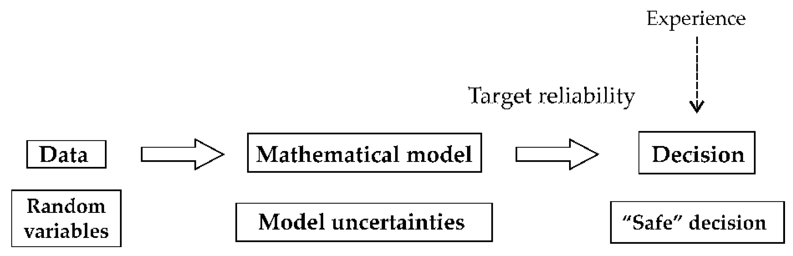
In limit states, model uncertainties can be considered as random variables to cover the imprecision and incompleteness of the relevant theoretical models for the resistance and load effects [27]; see Figure 1.

Although random input variables are given attention in experimental research, model uncertainties are often a neglected part of probabilistic and especially sensitivity analysis of reliability.

The importance of model uncertainties has been confirmed in numerous studies. Model uncertainties in the shear resistance of reinforced concrete beams were studied in [35,36]. The statistical analysis of model uncertainties was evaluated in [37] by comparing the resistance data from experiments and models of reinforced concrete members. The effects of model uncertainties on the shear resistance of recycled aggregate concrete elements were studied in [38]. A methodology for quantifying model uncertainties of reinforced concrete columns exposed to fire was published in [39]. The model uncertainties of the resistance of steel members under axial compression, bending and combined axial compression and bending were investigated in [40]. For composite structures, studies of resistance models have shown that model uncertainties for buckling are more significant than for flexure [41,42].

Model uncertainties are always present, because each building’s structure is unique, and measurements on many structures of the same type are impossible. Despite this importance, the existing knowledge about model uncertainties and their characteristics seems to suffer from imprecise definitions and a lack of available experimental data [28].

The careless introduction of model uncertainties can lead to an excessively reliable (uneconomical) design. On the contrary, neglecting these uncertainties can lead to an unsafe design. Therefore, they should be quantified very carefully.

There is a complete lack of research into model uncertainties using methods of global sensitivity analysis of P_f. This article attempts to fill this gap with research into ROSA building on [43]. The paper builds on available concepts [27]. The novelty of this work is the formulation of a new methodology for quantifying model uncertainties based on the proposed rule called “variance = entropy”.

2. Probability Analysis of Reliability with Model Uncertainties

The reliability theory is widely used to consider the uncertainties of engineering structures [1]. The general condition of reliability can be described using the limit state function in the form:

Z = f(X₁, X₂, …, X_M),

(1)

where X = (X₁, X₂, …, X_M) is a random input vector with M dimensionality, including the uncertain material characteristic, geometrical characteristics, loads and environmental factors. An example of building construction data is published, e.g., in [44]. The limit state function provides a failure criterion, where Z < 0 is the failure state and Z ≥ 0 is the safety state. The failure probability can be formulated as follows:

$$P_f=P\left(Z<0\right)=E\left(1_{Z<0}\right)=E\left(\frac{Z-\left|Z\right|}{2Z}\right),$$

(2)

where 1_Z<0 is a binary random variable, which has a value of 1 with the probability of failure P_f and 0 with the probability of success 1-P_f. The value of P_f is usually small (≈10⁻⁵) and must be lower than the target failure probability P_ft defined in standards [45].

In engineering practice, Equation (1) is usually written in the form of the limit state function of two random variables [46]:

$$Z=R-A,$$

(3)

where A is the load action, and R is the resistance. Reliability is generally expressed in probabilistic terms, where A and R are statistically independent random variables [45].

Eurocode [45] distinguishes two limit states at which the structure ceases to perform its intended function satisfactorily. The first limit state (ultimate limit state) deals with strength, overturning, sliding, buckling, fatigue fracture, etc. The second limit state (serviceability limit state) deals with discomfort to occupancy and/or malfunction caused by excessive deflection, crack width, vibration leakage and loss of durability. Both limit states are based on the general concept of action and barrier, where P_f can be calculated according to Equation (2). Structural reliability is verified by computational models using material and geometric characteristics with the application of various limits, such as stress limits [47,48], buckling limits [49,50], deformation limits [51,52], etc.

In Equation (1), the function f is usually not complete and accurate, so failure cannot be predicted without error, even if the statistical characteristics of all random input variables are known. The real outcome Z’ of the experiment can formally be written as:

Z’ = f^’(X₁, X₂, …, X_M, θ₁, θ₂),

(4)

where variables θ_i are additional random parameters containing the model uncertainties [27]. The model uncertainties account for random effects disregarded in models and simplifications in mathematical relationships.

Model uncertainties are ideally determined from a set of representative laboratory experiments and measurements on actual structures with measured and controlled values of X_i [27]. The model uncertainty in such cases is intrinsic in nature. Statistical uncertainty may be significant in the event of a small number of measurements (typical case in building structures). Furthermore, uncertainty may arise due to measurement errors of X_i and Z. In many cases, a good and consistent set of experiments is absent, and the statistical characteristics of model uncertainties are based solely on engineering judgement.

The probability that Z’ < 0 is formulated based on Equation (2) in the form:

$$P_f{}^{’}=P\left(Z^{’}<0\right)=E\left(1_{Z^{’}<0}\right)=E\left(\frac{Z^{’}-\left|Z^{’}\right|}{2Z^{’}}\right).$$

(5)

In engineering practice, most limit states are based on Equation (3), where X are continuous input random variables, and P_f, P_f’ are small.

When assessing the reliability of a structure, model uncertainties can be related to load effect models evaluating the effects of loads and their combinations or resistance models based on simplified relationships or complex numerical models. The most common way of introducing model uncertainties is by multiplying the model resistance and load effect by factors θ₁ and θ₂; see, e.g., [38,39]. Equation (3) can be rewritten as:

Z’ = R’ − A’ = θ₁·R − θ₂·A,

(6)

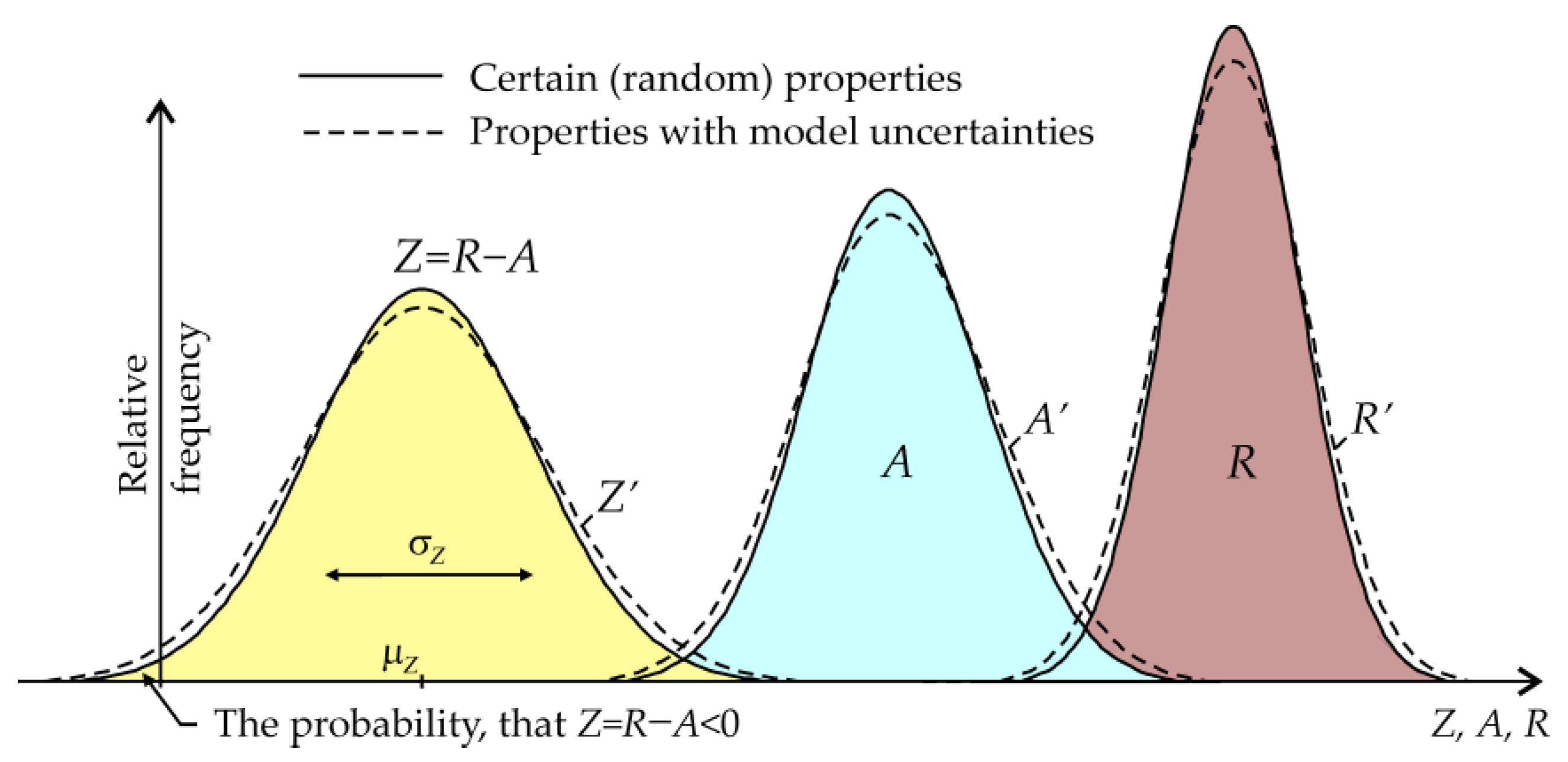
where θ₁ and θ₂ are model uncertainties. In Equation (6), a small variation coefficient is assumed for random variables θ₁, R, θ₂ and A [27,45]. It can be noted that common building structures have variation coefficients of R and A less than 0.2 [45]. The basic probabilistic models of model uncertainty θ₁ and θ₂ are listed in Table 3.9.1 in JCSS probabilistic model code [27]. For example, a bent steel member has a recommended lognormal probability density function (pdf) with a mean value of 1 and a standard deviation of 0.05 for both random variables θ₁ and θ₂ [27]. The lognormal pdf is introduced to exclude negative values rather than because of asymmetry since it differs slightly from the Gauss pdf. The main goal of such model uncertainties is to increase the variance (symmetric effect) of R and A; see Figure 2.

The probabilistic model code [27] suggests principles but does not provide details. In practice, there are several ways to account for model uncertainties in computational models; see, e.g., [28,53,54]. Although model uncertainties are justified in the conservative estimation of P_f, their use in sensitivity analysis is debatable. This is because random variables θ₁ and θ₂ are artificially added inputs, the nature of which must be separated from the basic random input vector X.

3. Reliability-Oriented Sensitivity Measures

The global ROSA aims at quantifying the influence of each input variable of a numerical model on the quantity of interest related to structural failure. The classical concept of global ROSA is based on the Sobol–Hoeffding decomposition of the variance of the Bernoulli distribution of 1_Z<0 [3,4].

$$V\left(1_{Z<0}\right)=P_f\cdot \left(1-P_f\right).$$

(7)

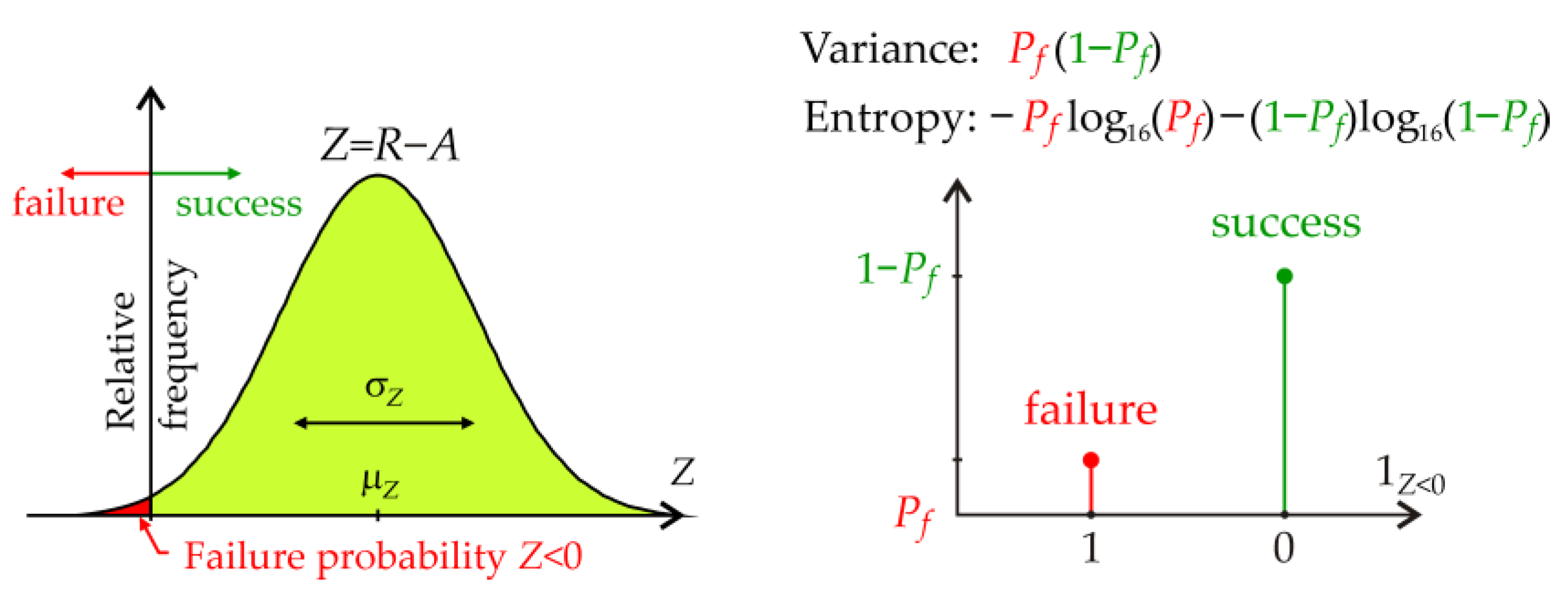
An alternative measure of uncertainty is entropy. The Shannon discrete entropy [55] of Bernoulli distribution of 1_Z<0 can be defined using the formula:

$$H\left(1_{Z<0}\right)=-P_f\cdot {\log }_b\left(P_f\right)-\left(1-P_f\right)\cdot {\log }_b\left(1-P_f\right).$$

(8)

In the Bernoulli distribution, Equations (7) and (8) depend only on P_f, as shown in Figure 3.

Entropy, by its very nature, only deals with the probabilities of each value, not the values themselves. The variance has this property because of its application to data 0 and 1, which are without units. However, the variance is generally dependent on values and units. Both measures maximise when each outcome occurs with the same probability, i.e., a lot of uncertainty, and minimise when there is only one outcome, i.e., no uncertainty. Both measures are measures of heterogeneity in the data 0 and 1.

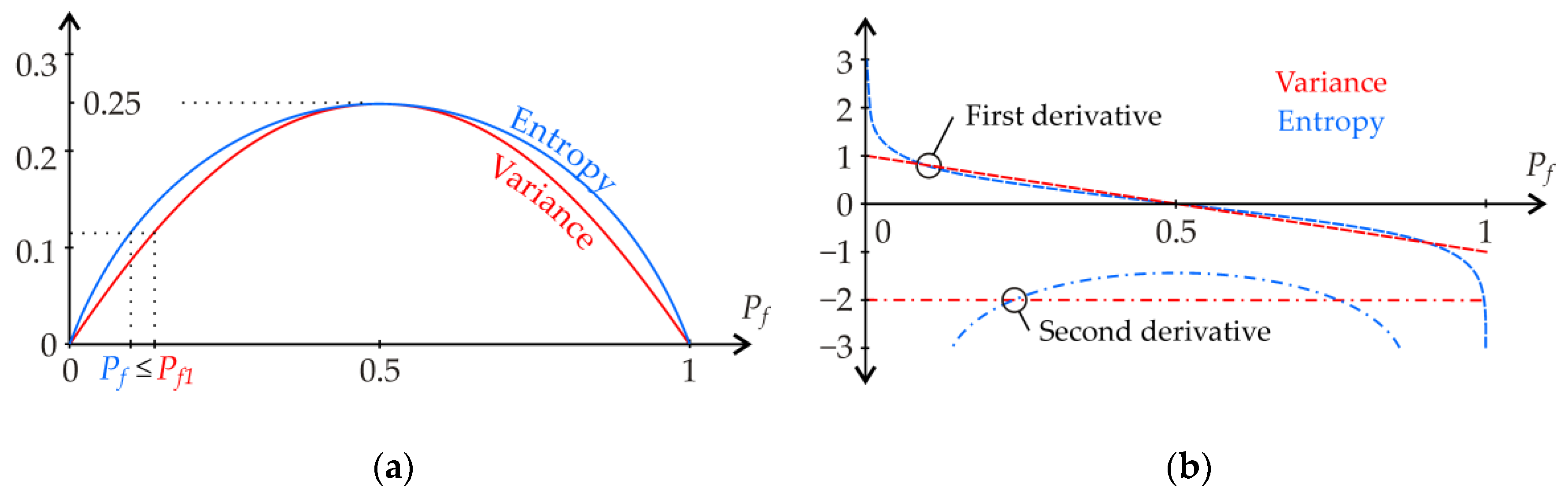
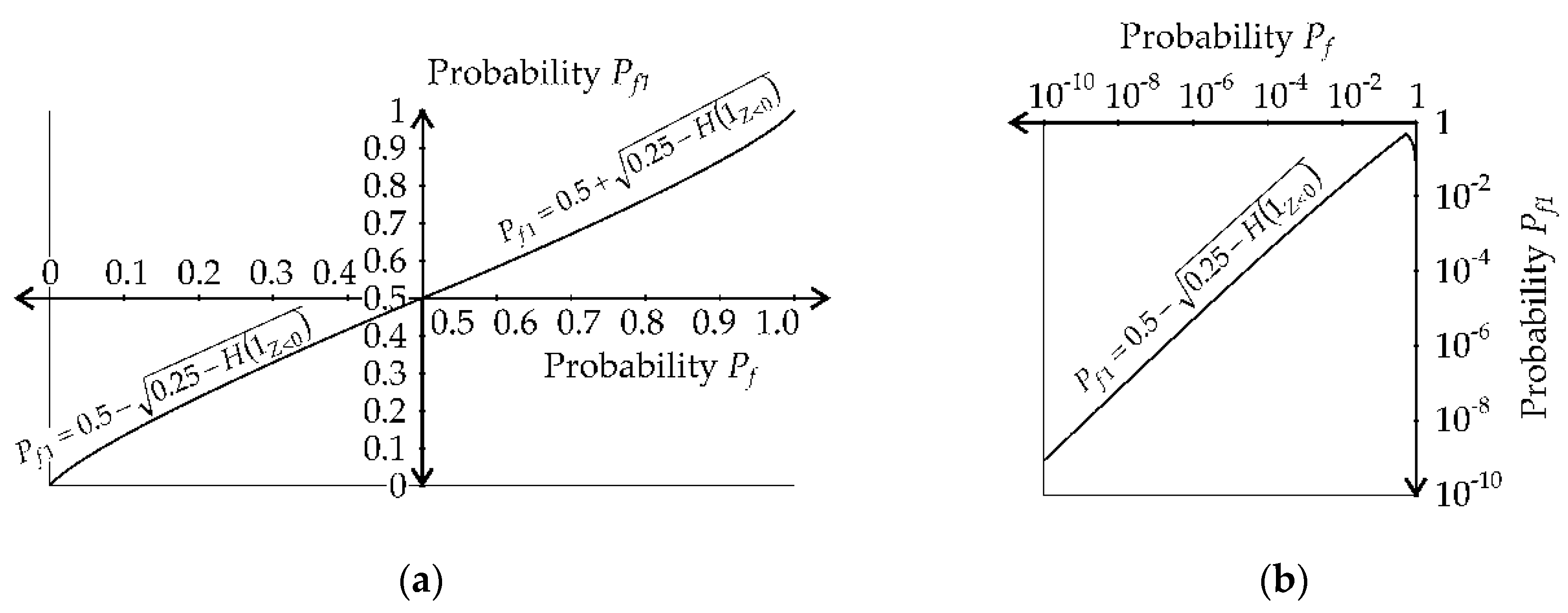
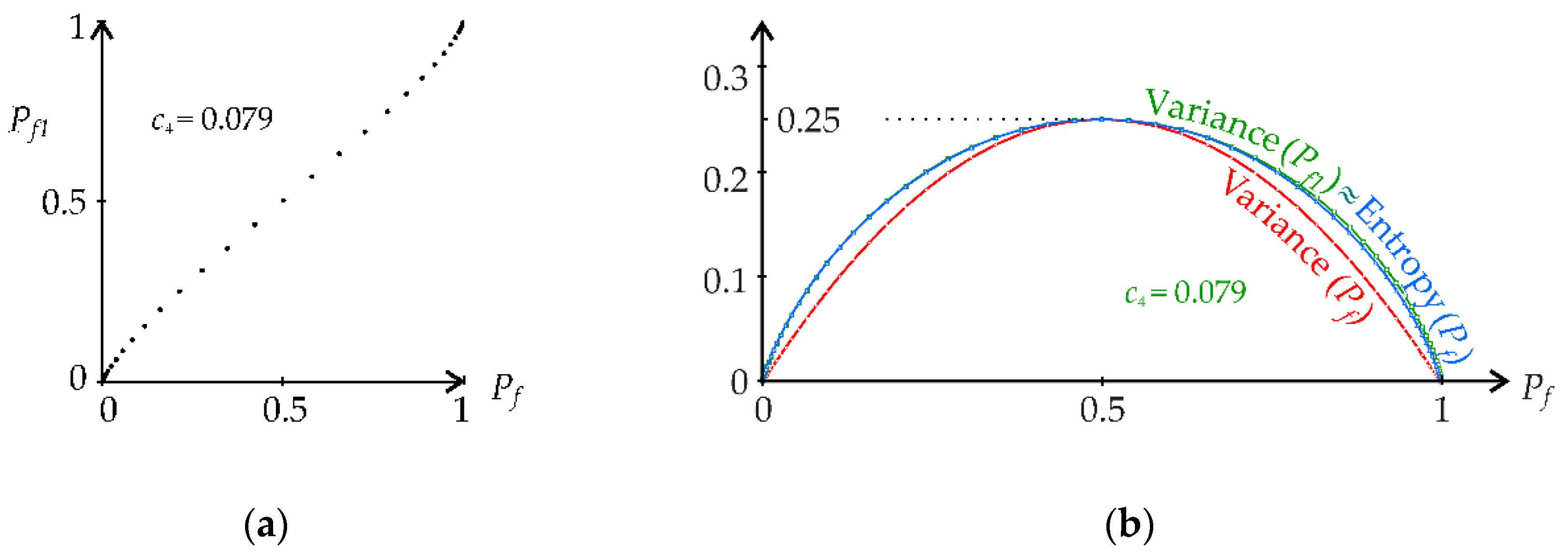
A comparison of the plots of Equations (7) and (8) is useful for logarithm base b = 16, where the rise of both domes is the same; see Figure 4a. For b = 16, the variance and Shannon entropy are similar in dome functions with a common peak point. On one level, the functions permit the increase of P_f to P_f1 for P_f < 0.5 or the decrease of P_f to P_f1 for P_f > 0.5. The input of the calculation is the value of P_f, which determines the level, and the output is P_f1 modified by the effects of model uncertainties; see Figure 4a. This is the same effect as the model uncertainties in the computational model and the same effect as the model uncertainty coefficients θ_i used in [27] for P_f < 0.5. For structural reliability analysis, the cases of P_f < 0.5 for small P_f values are of practical importance.

Although the domes are similar, the derivatives at the boundary points are different; see Figure 4b. Shannon entropy at point zero has each odd derivative ∞ and each even derivative −∞. At point one, all derivatives of Shannon entropy are −∞.

The “variance = entropy” rule increases P_f to P_f1 for P_f < 0.5; see Figure 4a. The rule is based on the formal similarity of the dome functions of entropy and variance of the Bernoulli distribution, where 0 and 1 are unitless. This is a new rule that has not yet been published and whose effectiveness is verified by the case studies presented in the next section. The rule in the presented form cannot be transferred to other types of distributions.

Entropic sensitivity analysis is a form of global sensitivity analysis. It decomposes the entropy of the output of a model or system into fragments that can be attributed to inputs or sets of inputs [43]. However, the fragments are not created by the decomposition of the variance as in Sobol. The global sensitivity analysis results are influenced only by the shape of the dome and not by its rise [43]. In practice, the sensitivity measure can be multiplied by a constant having a physical unit to obtain a different physical meaning.

Sensitivity indices based on entropy H(1_Z<0) can be written similarly to Sobol indices based on variance V(1_Z<0) [43]. For both sensitivity measures, the first-order sensitivity index (main effect) can be written in the form:

$$P_i=\frac{M\left(P_f\right)-E\left(M\left(P_f|X_i\right)\right)}{M\left(P_f\right)},$$

(9)

where M(P_f) = {V(1_Z<0), H(1_Z<0)}, but other sensitivity measures are also possible [43]. It is clear from Equation (9) that the amplitude of the measure in the numerator decreases with the amplitude in the denominator. Each measure can have a different amplitude. The sensitivity measure can be multiplied by a non-zero constant having a physical unit and assign physical meaning to the measurement. The second-order sensitivity index can be written as follows:

$$P_{ij}=\frac{M\left(P_f\right)-E\left(M\left(P_f|X_i,X_j\right)\right)}{M\left(P_f\right)}-P_i-P_j.$$

(10)

Higher-order sensitivity indices can be written analogously. However, the sum of all sensitivity indices must be equal to one.

$${\displaystyle \sum _i{P}_i}+{\displaystyle \sum _i{\displaystyle \sum _{j>i}{P}_{ij}}}+{\displaystyle \sum _i{\displaystyle \sum _{j>i}{\displaystyle \sum _{k>j}{P}_{ijk}}}}+\mathrm{...}+P_{\mathrm{123...}M}=1.$$

(11)

Sensitivity indices based on V(1_Z<0) are non-negative and less than one due to Sobol–Hoeffding decomposition [9,10]. Sensitivity indices based on H(1_Z<0) have not been proven to be non-negative and less than one, although this property has been observed in numerical studies [43].

The sensitivity indices can be non-negative and less than one in the specific case H(1_Z<0) = V(1_Z’<0), where Z’ has the same input vector X as Z, but the model uncertainties are added to Z’. The influence of model uncertainties can be considered in Z’ by (i) using added random variables θ_i or (ii) modifying Z to Z’ without added θ_i. Then, the sensitivity analysis is based on Sobol–Hoeffding decomposition V(1_Z’<0).

The current concept [27] assumes added model uncertainties as random variables θ_i, and other modifications of the limit state have not yet been introduced. Applying Equations (7) and (8), we can write:

H(1_Z<0) = V(1_Z’<0).

(12)

Upon substituting Equations (7) and (8) into Equation (12), we obtain:

$$-P_f\cdot {\log }_{16}\left(P_f\right)-\left(1-P_f\right)\cdot {\log }_{16}\left(1-P_f\right)=P_{f1}\cdot \left(1-P_{f1}\right),$$

(13)

where the left side is computed with P_f from Equation (3), and the right side introduces P_f1 taking into account model uncertainties according to (i) or (ii). The failure probability P_f1 can be obtained by solving Equation (13) in the form:

$$P_{f1}=\frac{1}{2}\mp \sqrt{\frac{1}{4}+P_f\cdot {\log }_{16}\left(P_f\right)+\left(1-P_f\right)\cdot {\log }_{16}\left(1-P_f\right)},$$

(14)

where the negative sign before the square root is for P_f $\le$ 0.5, and the positive sign is for P_f > 0.5. P_f $\le$ 0.5 is relevant for reliability analysis, where the increase from P_f to P_f1 can be performed by using random variables θ₁, θ₂ or using a specific limit state function Z’ without added random variables. The functional dependence of P_f1 on P_f has two very weakly non-linear (approximately linear) branches; see Figure 5a. Small failure probability values such as P_f ∈ [4.8 × 10⁻⁴, 8.5 × 10⁻⁶] are relevant for the structural reliability analysis; see the course in a lognormal scale in Figure 5b.

In the next section, the hypothesis that Equation (12) represents a good general condition for the modification of the limit state leading to rational model uncertainties θ₁ and θ₂, which have similar statistical characteristics to those recommended in [45], is studied.

4. Calibration of Models of Uncertainties

Why the entropic approach? If model uncertainty is added to the system, its entropy increases. Increasing the variance of R and A leads to H(1_Z<0) < H(1_Z’<0) and V(1_Z<0) < V(1_Z’<0); see Figure 2 and Figure 4a. Suppose the increase in entropy is similar for similar models. In that case, the increase in entropy can be a general rule for identifying model uncertainties as random variables in a stochastic model. The issue is the quantification of such an increase.

Let us focus on increasing the variance up to the entropy value according to Equation (12). Why this entropic approach? It will be shown in the case studies that the condition H(1_Z<0) = V(1_Z’<0) provides approximately the same model uncertainties as published in [27]. This phenomenon has not yet been published and is simply called “variance = entropy”. The following case studies verify and build on this phenomenon.

Numerous ways exist to introduce model uncertainties into the computational model to increase the variance. Practically applicable model uncertainties should be independent of P_f for easy implementation in common design situations, where design (target) failure probabilities are P_fd = {8.5 × 10⁻⁶, 7.2 × 10⁻⁵, 4.8 × 10⁻⁴} [45,56].

The entropy is equal to the variance if the added model uncertainties lead to P_f1, whereas without model uncertainties, it is P_f. Quantifying model uncertainties to achieve P_f1 is treated in case studies in several variants.

4.1. Models Uncertainties Based on Random Variables θ₁, θ₂

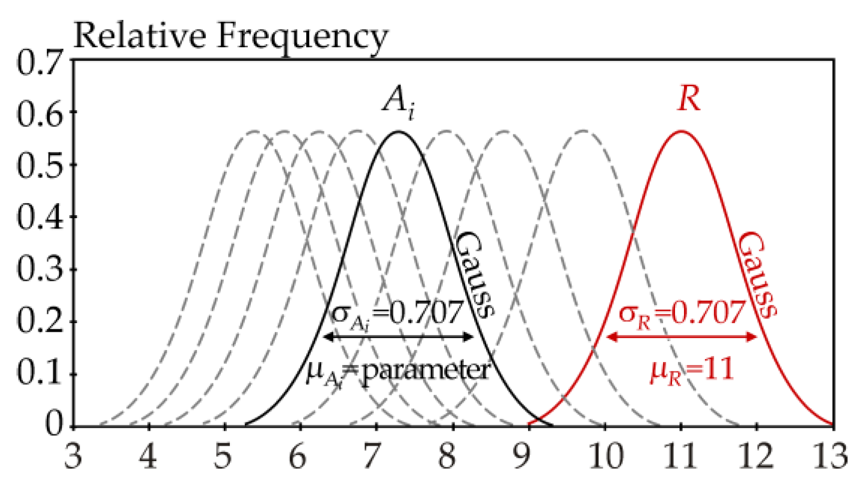
The concept of the case studies is illustrated in Figure 6. Random variable R (X₁) has a mean value μ_R = 11 and a standard deviation σ_R = 1/√2. Random variable A (X₂) has a mean value μ_A as a parameter and a standard deviation σ_A = σ_R. Both variables R and A have a Gauss pdf and are statistically independent; see, e.g., [23]. Then, random variable Z also has a Gauss pdf with a mean value μ_Z = 11 − μ_A and a standard deviation σ_Z = 1. The units of R and A are not important (they can be, e.g., kN); see Figure 6.

In the case studies, the control parameter μ_A decreases with a step of 0.05 and gradually has the values 11, 10.95, 10.9, etc. Depending on μ_A, P_f has the values 0.48, 0.46, 0.44, etc. P_f is estimated using numerical integration with a small step of ∆a taken over [μ_Z − 10σ_Z, μ_Z + 10σ_Z]. Although μ_A is the control parameter, the results of the case studies are shown in dependence on P_f, which is a more illustrative variable.

In the first case study, P_f1 is calculated using θ₁ and θ₂ as random variables in Equation (6). Random variables θ₁ and θ₂ are considered with a lognormal pdf with mean values μ_θ1 = μ_θ2 = 1. Standard deviations σ_θ1, σ_θ2 are output values that have to be found such that P_f’ ≈ P_f1, and σ_θ1 =σ_θ2. In practice, the procedure is as follows: the value of the input parameter μ_A is selected; subsequently, the value of P_f is estimated by numerical integration according to Equation (2); then, the value of P_f1 is calculated according to Equation (14). Next, the estimation of σ_θ1, σ_θ2 is performed numerically using the bisection method with an accuracy of 1 × 10⁻⁵ so that P_f’ converges to P_f1. Finally, the value of P_f’ is estimated according to Equation (5) using 10¹⁰ runs of the Monte Carlo method in each step of the bisection method. The output is the estimation of σ_θ1, σ_θ2, where σ_θ1 = σ_θ2. 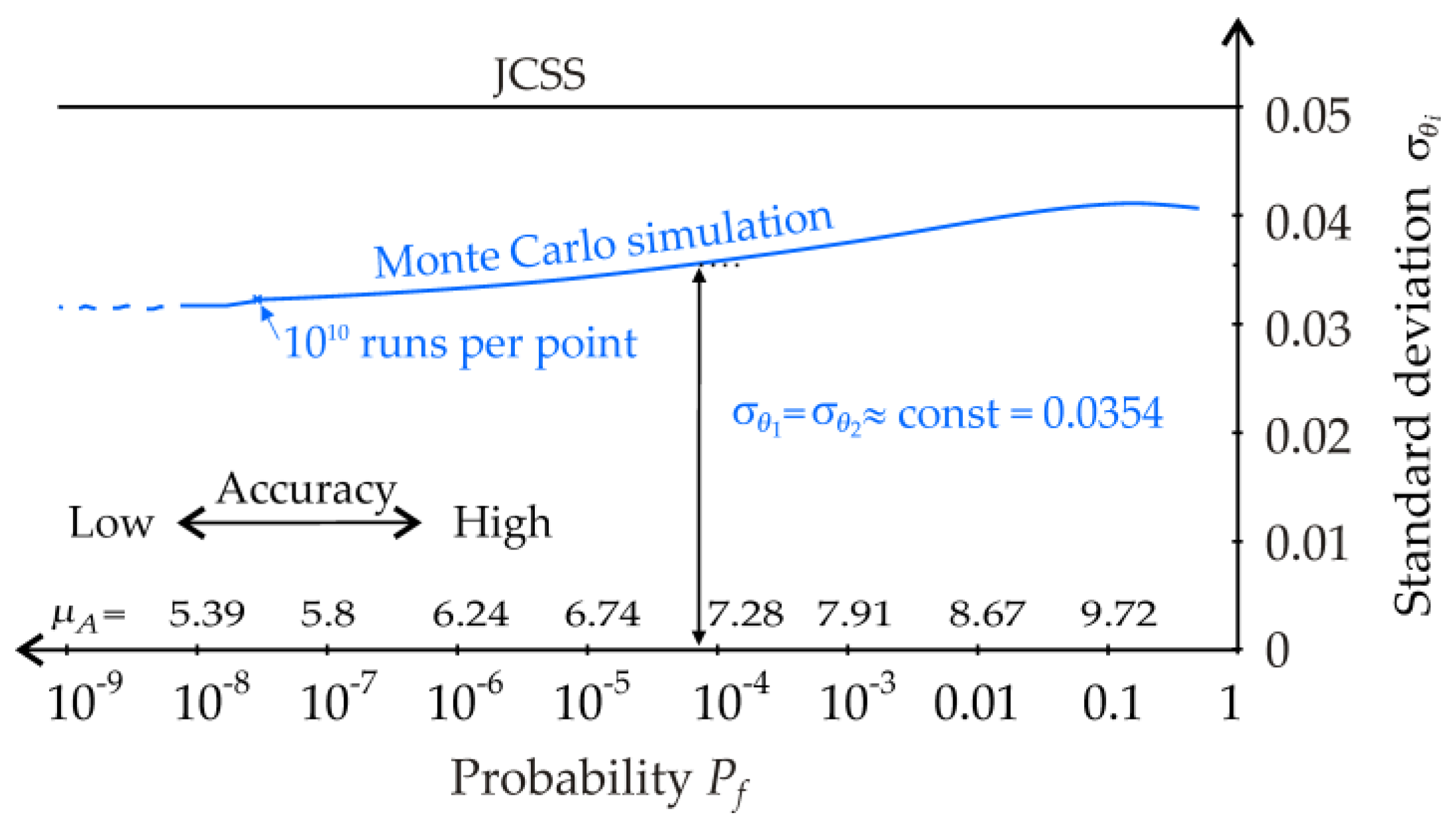The point (P_f, σ_θ) is depicted in the graph plotted in Figure 7. The blue line in Figure 7 is obtained by connecting 120 points (P_f, σ_θ), where one point is for one value of the control parameter μ_A.

The blue line in Figure 7 shows that the plot of the standard deviations can be approximately replaced by a constant value σ_θ1 = σ_θ2 = 0.0354, which is independent of P_f. The constant mean value and standard deviation permit the implementation of θ₁ and θ₂ into the computational model independently of P_f, which is a crucial requirement. Although the concept of [27] is based on the philosophy of constant moments μ_θi, σ_θi, the implementation of model uncertainties into a stochastic model is unclear.

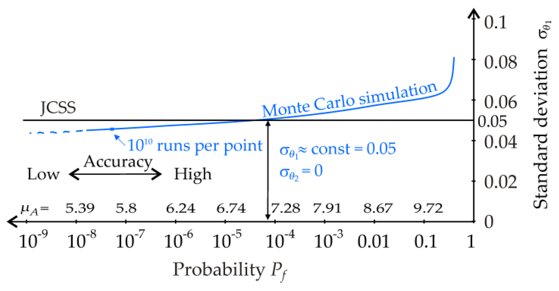
In the second case study, P_f1 is calculated using one random variable, θ₁, in Equation (6), whereas the second variable, θ₂ = 1, is deterministic. The results of the study are shown in Figure 8. It is apparent that the second model approximates the model uncertainties of [27] more closely. A comparison of Figure 7 and Figure 8 shows that a single random variable θ₁ can adequately describe the uncertainty in theoretical models.

Other ways of introducing model uncertainties have been explored and are possible. However, they are more problematic due to greater misaligned σ_θ1 and σ_θ2, according to P_f.

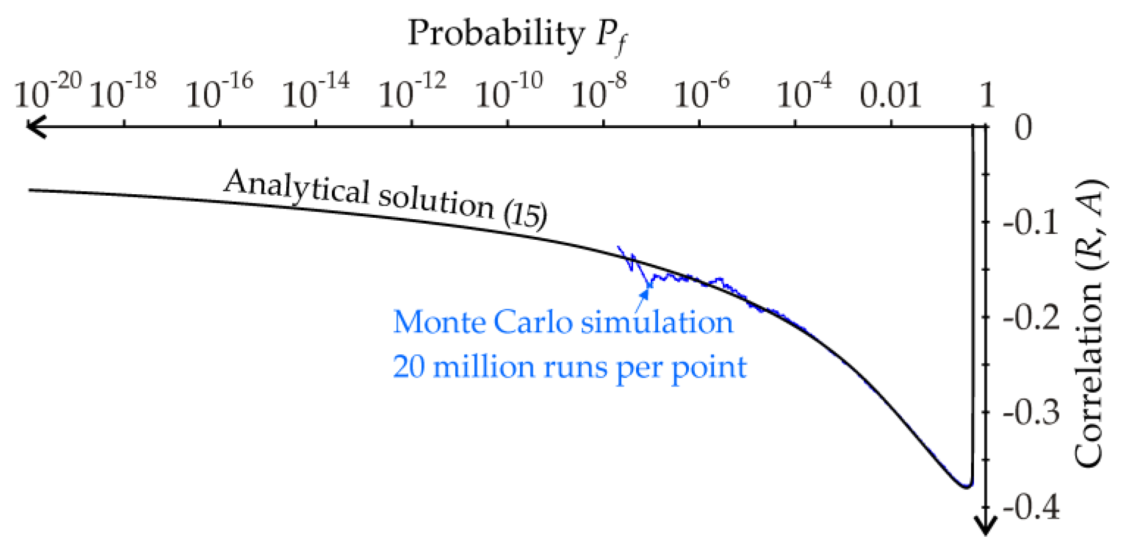
Throughout the article, R and A are statistically independent variables X₁ and X₂. In this case study, let R and A have artificially introduced weak correlation, and θ₁ and θ₂ are not considered. The joint pdf of correlated R and A with a Gauss pdf can be written as follows:

$$f_{RA}\left(r,a\right)=\frac{1}{2\pi {\sigma }_R{\sigma }_A\sqrt{1-{\rho }^2}}\exp \left(-\frac{{\left(\frac{r-{\mu }_R}{{\sigma }_R}\right)}^2-2\rho \left(\frac{r-{\mu }_R}{{\sigma }_R}\right)\left(\frac{a-{\mu }_A}{{\sigma }_A}\right)+{\left(\frac{a-{\mu }_A}{{\sigma }_A}\right)}^2}{2\left(1-{\rho }^2\right)}\right).$$

(15)

The estimate of P_f’ is computed as the numerical integral of Equation (15). In the outer loop, the pdf of A is numerically integrated with a small step ∆a taken over (μ_A − 10σ_A, μ_A + 10σ_A). In the inner loop, the pdf of R is numerically integrated with a small step ∆r taken over (μ_R − 10σ_R, a). The estimation of correlation corr(R, A) is performed with an accuracy of 1 × 10⁻⁵ using the bisection method, with the goal of P_f’ → P_f1. The blue line shows the control calculation, where P_f’ is estimated using the Monte Carlo method; see Figure 9.

The course of the correlation is non-linear and strongly dependent on P_f. Therefore, the introduction of negative corr(R, A) is an inappropriate implementation of model uncertainties into stochastic models. Moreover, R and A are products of their stochastic models with their random variables. Therefore, the artificial introduction of a correlation between R and A has no basis in real limit states.

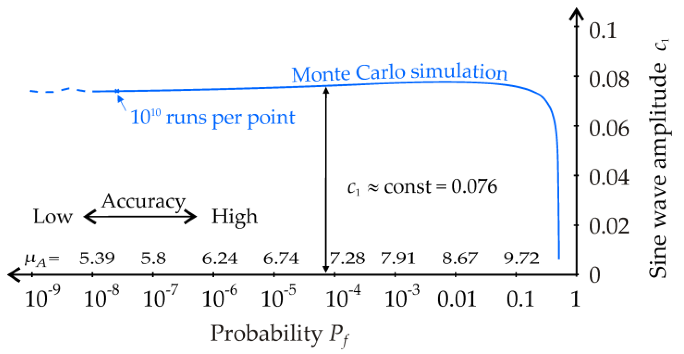
4.2. Model Uncertainties Based on Pseudorandom Sequences in Monte Carlo Techniques

Increasing the failure probability can be achieved within the limit state function without added random variables θ_i. Failure occurs if Z’ < 0, where Z’ is the limit state function supplemented by the influence of model uncertainties in the pseudorandom form.

In the first case, the pseudorandom effect [·] is introduced in the form:

$$Z^{’} =R^{’} - A^{’} = R\left[1+c_1\cdot \sin \left(c_0\frac{A}{R}\right)\right]-A,$$

(16)

where c₀ and c₁ are deterministic variables, c₀ is a large number, e.g., 10⁹σ_Z (but not infinity), and c₁ is the amplitude of the sine function. The goal is to calibrate the amplitude c₁ so that Pf’ = P_f1. The size of c₁ is sought using the bisection method with an accuracy of 1 × 10⁻⁵ so that P_f’ converges to P_f1. The value of P_f’ is estimated according to Equation (5) using 10¹⁰ runs of the Monte Carlo method in each step of the bisection method. The output of the procedure is an estimate c₁. Estimation of the values of P_f and c₁ is performed 120 times using parameter μ_A step-by-step according to the method described in the preceding section. Finally, the dependence of c₁ vs. P_f is plotted by joining 120 points (P_f, c₁); see Figure 10.

The blue line in Figure 10 shows that the course of c₁ can be approximately replaced by a constant value c₁ = 0.076 so that c₁ is independent of P_f. The model uncertainty in Equation (16) is based on the product [·] of two random numbers A/R without added θ_i. For the Monte Carlo method, we can write:

$$P_f{}^{’}=P\left(Z^{’}<0\right)\approx \frac{1}{N}{\displaystyle \sum _{j=1}^N{1}_{a_{\mathrm{j}}>r_j\left[1+c_1\cdot \sin \left(c_0 a_{\mathrm{j}}/r_j\right)\right]}},$$

(17)

where N is the number of runs of the Monte Carlo method, a_j, r_j are random realisations of A and R, and c₀, c₁ are deterministic variables. The numerical results are the same irrespective of whether a_j/r_j or r_j/a_j is used. The product [·] based on the sine function is close enough to the pseudorandom number and suits the intended use. It can be shown that substituting c₀·A/R for the third independent random variable in sin (·) does not affect the result shown in Figure 10.

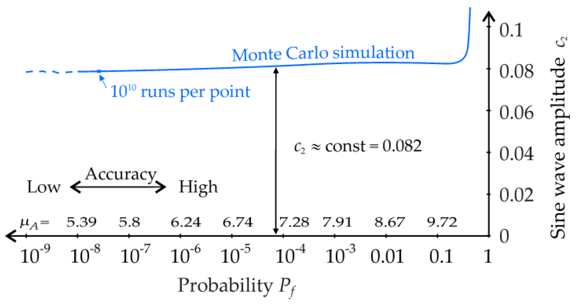
In the second case, the pseudorandom number is introduced as a multiple of random variable A:

$$Z^{’} = R^{’} -A^{’} = R-A\left[1+c_2\cdot \sin \left(c_0\frac{R}{A}\right)\right].$$

(18)

Calibration is performed according to the procedure described in the previous paragraph, but for variable c₂. The graph of c₂ vs. P_f is shown in Figure 11.

In order to have c₂ independent of P_f, the course of c₂ can be approximated by a constant value of c₂ = 0.082.

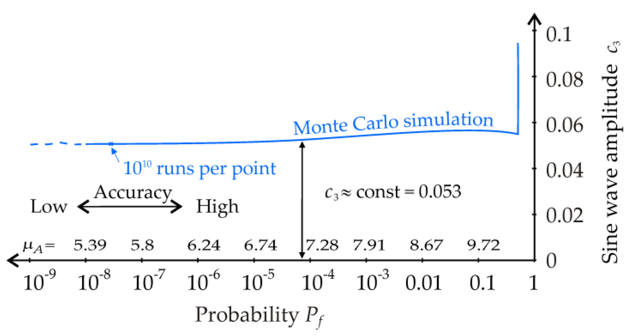
In the third case, the pseudorandom number is introduced as a multiple of both random variables A and R in the form:

$$Z^{’} = R^{’}-A^{’} = R\left[1+c_3\cdot \sin \left(c_0\frac{A}{R}\right)\right]-A\left[1+c_3\cdot \sin \left(c_0\frac{R}{A}\right)\right],$$

(19)

where c₃ is calibrated using the procedure described in the preceding studies. The course of c₃ can be approximated by a constant value of c₃ = 0.053; see Figure 12.

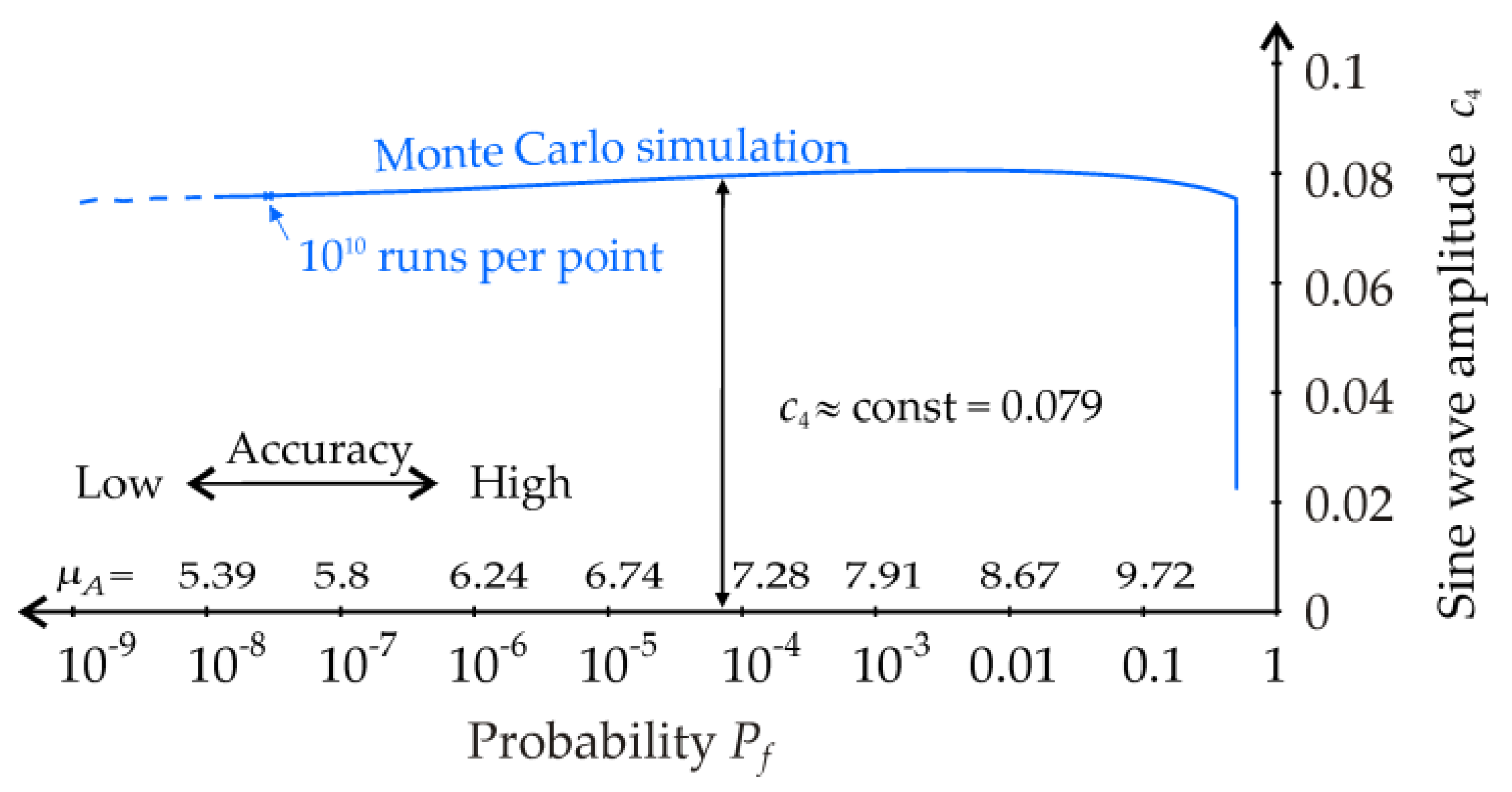
The fourth case introduces model uncertainties by rewriting the reliability condition Z $\ge$ 0 in the logarithmic form as follows:

$$Z=R-A\ge 0\Rightarrow \frac{R}{A}\ge 1.$$

(20)

The logarithmic condition of reliability Γ $\ge$ 0 is based on the transformation

$$\mathsf{\Gamma }=\ln \left(\frac{R}{A}\right)\ge \ln \left(1\right)\Rightarrow \mathsf{\Gamma }=\ln \left(R\right)-\ln \left(A\right) \ge 0,$$

(21)

where model uncertainties can be introduced as pseudorandom fluctuations around zero using the sine function as follows:

$$\ln \left(R\right)-\ln \left(A\right) \ge c_4\cdot \sin \left(c_0\frac{R}{A}\right)\Rightarrow {\mathsf{\Gamma }}^{’}=\ln \left(R\right)-\ln \left(A\right) -c_4\cdot \sin \left(c_0\frac{R}{A}\right)\ge 0.$$

(22)

The graph of c₄ vs. P_f is analysed using the procedure described in the preceding studies; see Figure 13. The course of c₄ can be approximated by the constant value c₄ = 0.079 at the point P_f = 10⁻⁵; see Figure 13. It can be noted that removing the logarithms in Equation (22) does not lead to the parameter c₄ with alignment course, and therefore the study is not presented.

By introducing P_f independent constants c₄ = 0.079 and c₀ = 10⁹ into Equation (23), the relationship for estimating P_f1 ≈ P_f’ using the Monte Carlo method can be written as:

$$P_f{}^{’}=P\left({\mathsf{\Gamma }}^{’}<0\right)=E\left(1_{{\mathsf{\Gamma }}^{’}<0}\right)\approx \frac{1}{N}{\displaystyle \sum _{j=1}^N{1}_{\ln \left(r_j\right)-\ln \left(a_{\mathrm{j}}\right) <0.079\cdot \sin \left({10}^9{r}_j/a_{\mathrm{j}}\right)}},$$

(23)

where N is the number of runs of the Monte Carlo method, and a_j and r_j are random realisations of A and R. The results in Figure 14 are treated similarly to the preceding studies, but with the output P_f1. Points P_f1 are calculated for thirty steps of parameter μ_A, where 10¹⁰ steps of the Monte Carlo method are used in each step to estimate P_f1; see Figure 14.

For P_f < 0.5, it holds that P_f1 > P_f. For P_f > 0.5, it holds that P_f1 < P_f; see Figure 14a. It can be summarised that the entropy H(1_Z<0) = H(1_Γ<0) can be approximated by the variance V(1_Γ’<0) based on P_f1 = E(1_Γ’<0) as follows:

$$-P_f\cdot {\log }_{16}\left(P_f\right)-\left(1-P_f\right)\cdot {\log }_{16}\left(1-P_f\right)\approx P_{f1}\cdot \left(1-P_{f1}\right).$$

(24)

The approximation of the left half of the dome, P_f < 0.5, is more accurate because c₄ = 0.079 was calibrated for the point P_f = 7.2 × 10⁻⁵; see Figure 14b.

The approximation of the other cases H(1_Z<0) ≈ V(1_Z’<0) based on Z’ can be presented analogously. Figure 10, Figure 11, Figure 12 and Figure 13 show the constants c₁ to c₄ subtracted from the point P_f = 7.2 × 10⁻⁵, representing the common design condition of a building structure [45].

Although pseudorandom sequences can introduce the influence of model uncertainties without added random variables θ_i, they require the introduction of deterministic parameters, which is not very practical.

4.3. Summary

Case studies 1 and 2 have shown that the “variance = entropy” rule converges to the model uncertainty θ_i recommended in [27]. The model uncertainties θ_i have approximately constant statistical characteristics for any P_f < 0.5.

Thus, a reliability assessment including the effect of model uncertainties is possible by calculating P_f1 from P_f, where P_f is failure probability computing without model uncertainties. The failure probability P_f1, including the effect of model uncertainties, is calculated from Equation (25):

$$P_{f1}=\frac{1}{2}-\sqrt{\frac{1}{4}+P_f\cdot {\log }_{16}\left(P_f\right)+\left(1-P_f\right)\cdot {\log }_{16}\left(1-P_f\right)}\le P_{ft}$$

(25)

where P_ft is the target (design) failure probability, e.g., 7.2 × 10⁻⁵ [45]. The design of a structure is safe if P_f1 $\le$ P_ft. The rule is called “variance = entropy”. This is a simple yet effective rule taking into account the influence of model uncertainties without adding random variables θ_i to the stochastic computational model.

This direct application of the “variance = entropy” rule can be recommended for practical use. The advantage of this approach is that both probabilistic and sensitivity analysis are performed in the usual way with only nature random input variables.

5. Global Sensitivity Analysis of Reliability with Model Uncertainties

The influence of model uncertainties and random input variables can be investigated using global ROSA. In the preceding section, the global sensitivity analysis of P_f was performed using μ_R = 11, μ_A = 8.6735 and σ_R = σ_A = 1/√2. Using these parameters, P_f = 0.01 and P_f1 = 0.02.

In Equation (11), the estimation of sensitivity indices P_i, P_ij, etc. is based on the unconditional and conditional estimates of P_f. The unconditional estimate of P_f used ten million MC runs. The conditional estimate of P_f∣X_i used one hundred thousand MC runs, and the estimate of E(M(·)) used one hundred thousand MC runs. Higher-order sensitivity indices are estimated analogously with the same number of runs.

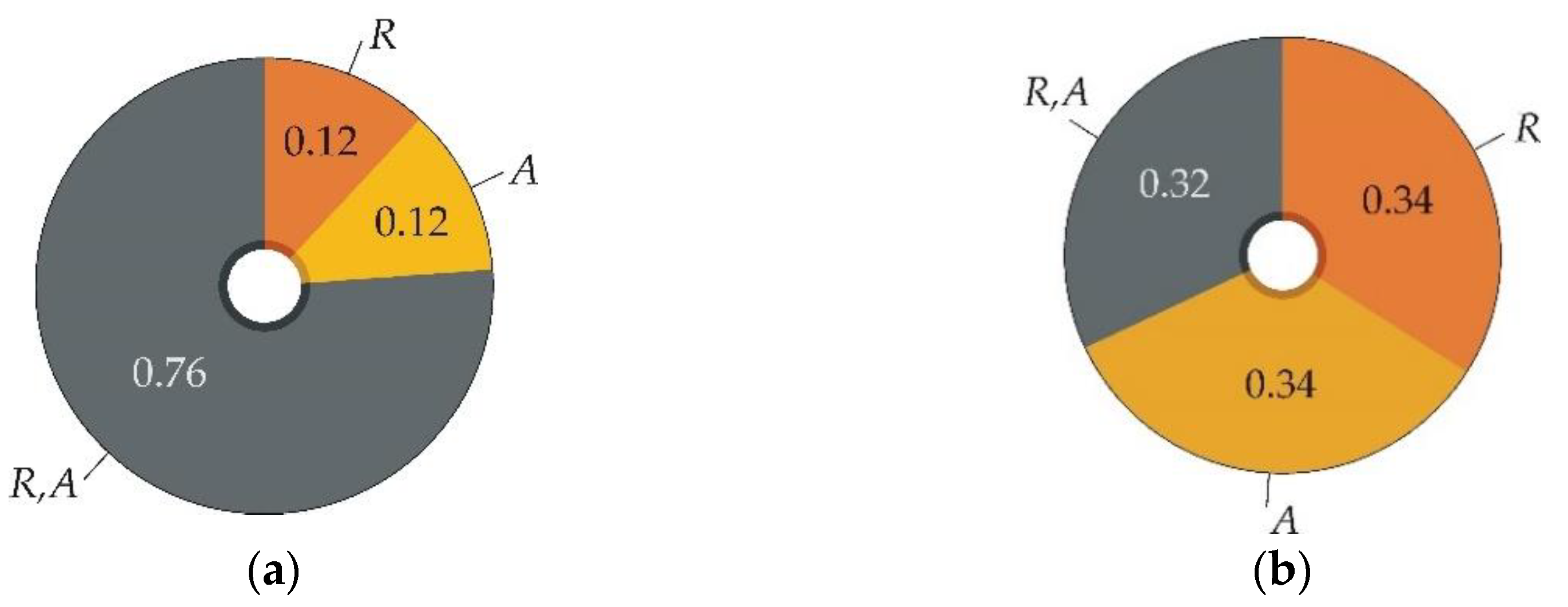
The sensitivity analysis results shown in Figure 15 are based on the Sobol–Hoeffding decomposition of variance V(1_Z<0) [3,4] and the fragmentation of Shannon entropy H(1_Z<0) introduced in [43]; see Figure 15. The sensitivity indices shown in Figure 15 do not consider the influence of model uncertainties.

The sensitivity indices in Figure 16 are based on the decomposition of the variance V(1_Z’<0) but using a modified function of the limit state Z’. The results in Figure 16a are obtained from Equation (6), where both θ₁ and θ₂ have a lognormal pdf with μ_θ1 = μ_θ2 = 1 and σ_θ1 = σ_θ2 = 0.0354. The results in Figure 16b are obtained from Equation (22) with parameters c₀ = 10⁹ and c₄ = 0.079. The other variants of Z’ lead to results close to Figure 16b.

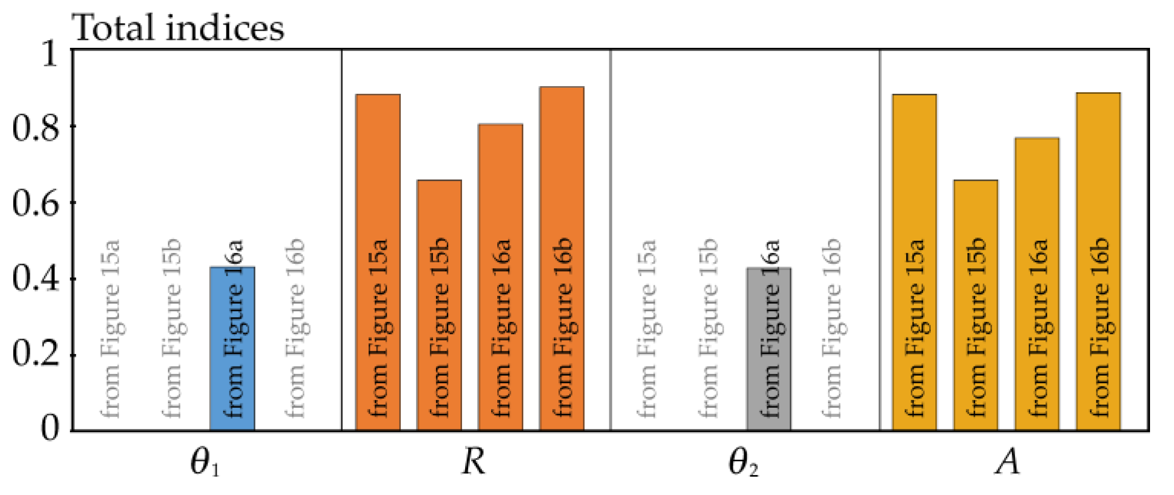
The sensitivity ranking can be determined using total sensitivity indices [57]. The total index measures the contribution to the output variance (entropy) of X_i, including all variance (entropy) caused by its interactions, of any order, with any other input variables. For input random variables R (X₁) and A (X₂), the total index can be written as P_1T = P₁ + P₁₂ and P_2T = P₂ + P₁₂. Total indices are particularly desirable when multiple input random variables with a high proportion of interaction effects are analysed using higher-order indices; see Figure 16a. It can be noted that global sensitivity analysis of small failure probability values has a high proportion of interaction effects when the sensitivity measure is variance [43]. The total indices in Figure 17 are calculated from the sensitivity indices in Figure 15 and Figure 16.

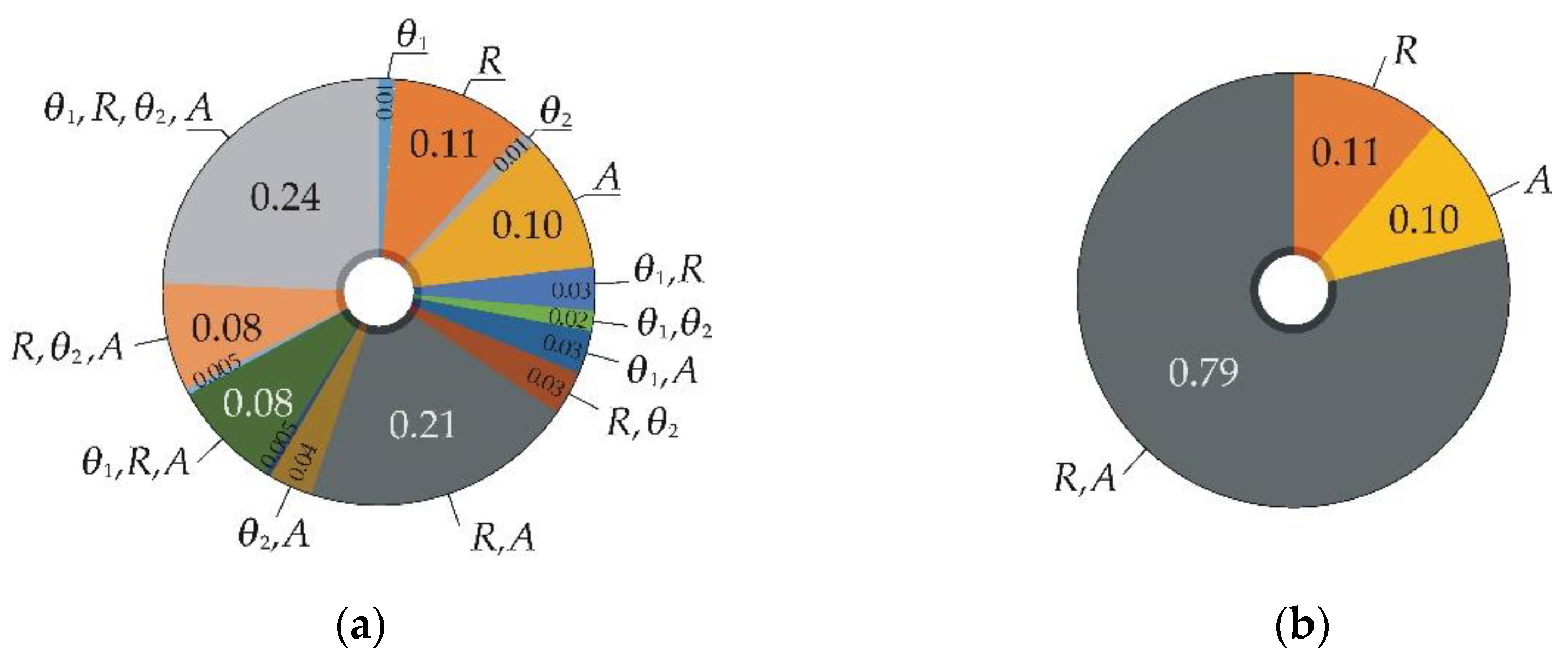
Figure 15 shows the symmetric influence of variables R and A. Figure 16 shows a slightly more significant influence of variable R (compared to A) due to the slightly asymmetric influence of model uncertainties introduced into Z’. The differences between the total indices of R and A are negligible for the same Z’; see Figure 17. Figure 16a presents multiple sensitivity indices and interaction effects due to model uncertainties θ₁ and θ₂ introduced as random variables. The influence of θ₁ and θ₂ is relatively large and reaches half of the effects of R and A; see the third column in Figure 17. In the case of a larger number of inputs, random variables θ₁ and θ₂ may overshadow the influence of the weakest input variables.

6. Global Sensitivity Analysis Based on Rényi Entropy

In this chapter, the results shown in Figure 15b are evaluated using Rényi entropy [58]. The same statistical characteristics μ_R = 11, μ_A = 8.6735, and σ_R = σ_A = 1/√2 are used.

The theoretical background on Rényi entropy can be found in [59,60]. Rényi entropy is one of the extensions of the Shannon entropy from Equation (8). For a binary random variable, the relationship of Rényi entropy can be written as:

$$H_{\alpha }\left(1_{Z<0}\right)=\frac{1}{1-\alpha }{\log }_b\left(P_f^{\alpha }+{\left(1-P_f\right)}^{\alpha }\right).$$

(26)

where α is the order of Rényi entropy, $\alpha \ge 0$ and $\alpha \ne 1$. The limit for α → 1 is Shannon entropy. Other properties of the Renyi entropy can be found, e.g., in [61].

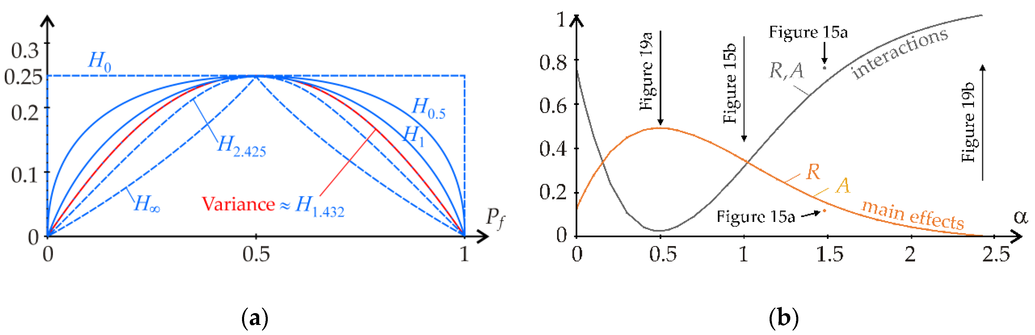
Figure 18a depicts Rényi entropy for the logarithm base b = 16 and α ∈ {0, 0.5, 1, 1.432, 2, ∞}. The variance can be approximated by the Rényi entropy for α ≈ 1.432, where the value of the entropy with its first derivative approximately coincides with the value of the variance and its first derivative. However, the sensitivity indices from Rényi entropy with α = 1.432 differ slightly from Figure 15a. Sensitivity indices for α ∈ [0, 2.425] are depicted in Figure 18b.

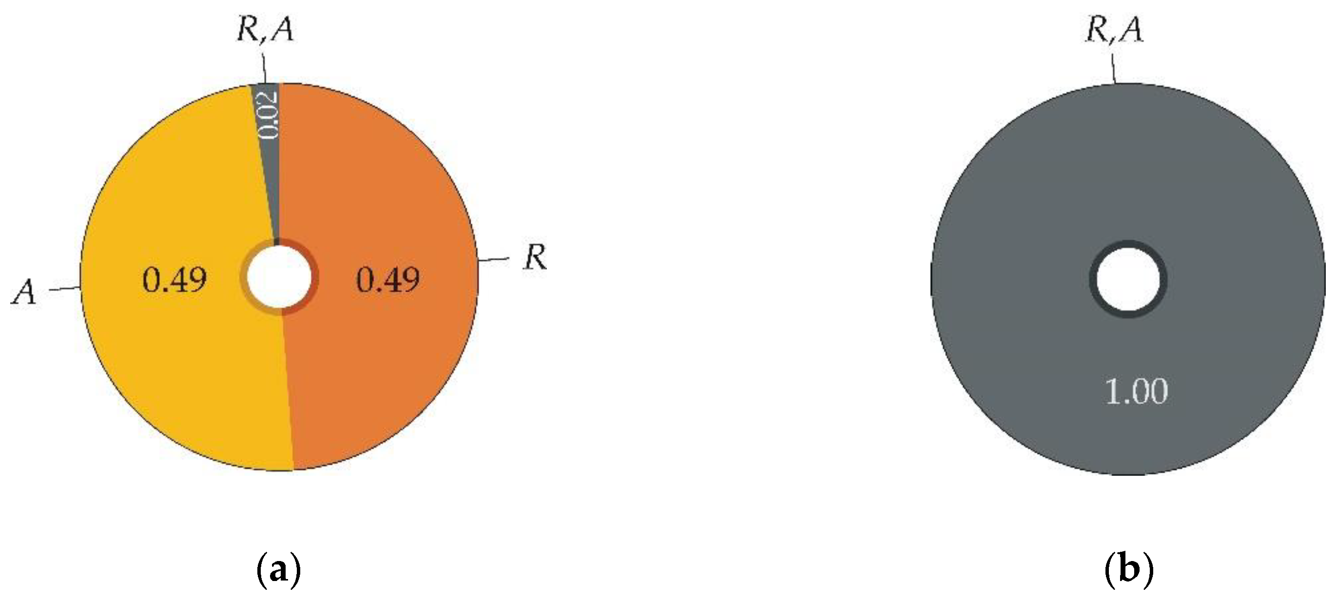
Figure 18b shows that the parameter α significantly changes the ratio of the first- and second-order sensitivity indices. The first-order sensitivity indices are maximum for α ≈ 0.5; see Figure 19a. The second-order sensitivity indices (interaction effects) are equal to one, and the first-order sensitivity indices (main effects) are equal to zero for α ≈ 2.425; see Figure 19b. The first-order sensitivity indices become negative, and the second- (last) order sensitivity index becomes greater than one for α > 2.425.

The example shows the sensitivity measure’s significant influence on the sensitivity indices’ structure. The sensitivity order of R and A is equal in all cases, but specific values of α provide this information using a large proportion of first-order sensitivity indices (see Figure 19a), whereas others express the same result in an avant-garde way; see Figure 19b.

7. Discussion

Entropy and variance have been investigated in case studies in which the limit states were described using a Bernoulli random variable. Model uncertainties were calibrated from the condition that Shannon entropy is approximated by the variance P_f’ (1 − P_f’) ≈ −P_f log₁₆(P_f) − (1 − P_f)log₁₆(1 − P_f), where P_f’ is the increased value of failure probability due to model uncertainties. Studies have shown that increasing the variance to the entropy value can be achieved by using model uncertainties with statistical characteristics approximately according to the recommendations in [27].

Model uncertainties θ_i are given for models of building structures, where R and A may depart from the Gaussian distribution due to the small skewness and kurtosis values [62]. The statistical characteristics of θ_i are approximately the same if the coefficients of variation R and A are small, which is in accordance with [45]. Under these assumptions, R and A can be the product of other data of the building structure (parameters of the computational model), such as load cases [56] or material and geometric characteristics of structures; see, e.g., [44,63].

The limit state Z without model uncertainties gives sensitivity analysis results with a perfectly symmetrical influence of R and A; see Figure 15. The classic Sobol sensitivity analysis based on the variance of Bernoulli distribution has a high proportion of interaction effect of R and A; see Figure 15a. The smaller the analysed P_f, the greater the interaction effects [23,43]. Distinguishing the effects of R from A can be difficult for very small P_f, where the interaction effect is strong (converges to one), and the main effects are weak (converges to zero).

Entropy offers a new sensitivity measure for the sensitivity analysis of small values of P_f. With a strong proportion of first-order indices, the entropy results approach the outputs, which are common in the application of Sobol sensitivity analysis of model outputs [57].

Taking into account model uncertainties as random variables θ₁ and θ₂ allows us to clarify the proportionality of the influence of both groups. Sensitivity analysis is important in terms of transparency of decision making, because then it is clear which reducible uncertainties have been left unchanged by our decisions [24]. On the other hand, the modified limit states Z’ with hidden model uncertainties give the sensitivity analysis results more clearly solely from the basic input variables without artificially added effects θ₁, θ₂.

The global ROSA based on entropy does not emanate from the Sobol–Hoeffding decomposition of the variance. The sum of all indices is one, but the indices need not be in the interval [0, 1]. The case study showed that the sensitivity indices based on Rényi entropy could be negative for entropy smaller than the variance. Sensitivity indices based on Shannon entropy have non-negative indices observed in case studies of common engineering tasks [43]. However, the possibility of negative indices does not affect the ability of the indices to identify the sensitivity ranking by comparing indices from lowest to highest.

When the number of random input variables is large, the sensitivity ranking can be determined using first-order indices and total indices, as with Sobol indices [57]. Practically, there is no need to calculate all 2^M − 1 indices, but only 2M indices are needed.

The approximation of the entropy by the variance V(1_Z’<0) ≈ H(1_Z<0) or V(1_Γ’<0) ≈ H(1_Γ<0) in the modified limit state was achieved by artificially adding model uncertainties to the original limit state Z or Γ. The approximation does not lead to the similarity of the sensitivity indices of variance and entropy. The sensitivity indices based on the decomposition V(1_Z’<0) or V(1_Γ’<0) remain close to Sobol; see the comparison of Figure 16b with Figure 15a. Although model uncertainties lead to a conservative estimate of the probability of failure, they do not replace the entropic sensitivity measure H(1_Z<0) in global sensitivity analysis. The properties of the entropic sensitivity measure were not replicated within the limit state function. The differences between the two sensitivity measures have not yet been explained. The entropic sensitivity measure remains the original sensitivity measure, which gives a good structure of sensitivity indices with a strong representation of first-order sensitivity indices.

The introduction of Rényi entropy in global ROSA showed the sensitivity indices’ dependence on the sensitivity measure’s shape; see Figure 18. The correct setting of parameter α leads to a good structure of sensitivity indices with high first-order effects, whereas the other cases have a large proportion of higher-order effects. The sensitivity index of the last order practically complements the indices of lower orders so that the sum of all indices in Equation (11) is one. If the sensitivity indices are estimated numerically with limited accuracy, then a high value of the sensitivity index of the last order may complicate the determination of the sensitivity ranking.

8. Conclusions

This article deals with the role of model uncertainties in sensitivity and probabilistic reliability analysis. The failure probability P_f was studied using the variance and entropy of the Bernoulli distribution with a binary outcome.

Introducing model uncertainties into a computational model increases the entropy of the system. Introducing model uncertainties in the magnitudes according to the recommendation of [27] increases the variance to the value of Shannon entropy. Shannon entropy is a good sensitivity measure useful for quantifying model uncertainties.

The “variance = entropy” approach presents a sufficiently sensitive and general rule for calibrating model uncertainties of any computational model. The rule increases the failure probability to a safer value, similar to using the model uncertainty factors from [27]. Such a new rule may benefit complex computational models for which recommendation [27] lacks detail. The accurate calibration of model uncertainties is useful, because their inappropriate introduction into a computational model can lead to a less optimal structural design due to a rough estimate of the failure probability.

Shannon entropy provides a useful sensitivity measure, especially for small values of P_f. Rényi entropy presents a sensitivity measure with great flexibility that significantly changes the sensitivity indices’ structure but does not change the information gained from sensitivity analysis. Rational results of sensitivity indices were obtained for dome functions between variance and Shannon entropy.