Article

Estimation of Citarum Watershed Boundary’s Length Based on Fractal’s Power Law by the Modified Box-Counting Dimension Algorithm

Department of Mathematics, Faculty of Mathematics and Natural Sciences, Universitas Padjadjaran, Sumedang 45363, Jawa Barat, Indonesia
*
Author to whom correspondence should be addressed.
Mathematics 2023, 11(2), 384; https://doi.org/10.3390/math11020384
Submission received: 12 December 2022 / Revised: 28 December 2022 / Accepted: 9 January 2023 / Published: 11 January 2023
(This article belongs to the Special Issue Advances in Fractals)

Abstract

:
This research aimed to estimate the length of the Citarum watershed boundary because the data are still unknown. We used the concept of fractal’s power law and its relation to the length of an object, which is still not described in other research. The method that we used in this research is the Box-Counting dimension. The data were obtained from the geographic information system. We found an equation that described the relationship between the length and fractal dimension of an object by substituting equations. Following that, we modified the algorithm of Box-Counting dimension by consideration of requiring a high-resolution image, using the Canny edge detection so that the edges look sharper and the dimension values are more accurate. A Box-Counting program was created with Python based on the modified algorithm and used to execute the Citarum watershed boundary’s image. The values of ε and N were used to calculate the fractal dimension and the length for each scale by using the value of C = 1 , assuming the ε as the ratio between the length of box and the length of plane. Finally, we found that the dimension of Citarum watershed boundary is approximately 1.1109 and its length is 770.49 km.

1. Introduction

As a branch of mathematics, fractal geometry has been used many times to describe the complexity of natural patterns and phenomena [1]. The word fractal has been popularized since 1975 by Mandlebrot and it comes from the Latin word fractus, which means an object with an irregular shape pattern [2]. Based on history, research on fractals began with Britain’s coastline as the first object [3]. The purpose of the research is to estimate the length of Britain’s coastline using the yardstick method, which was later known to have dimensions of 1.25 [4]. This method was used to count the number of segmentations with several sizes. Based on the research, the dimension is defined as mathematical measure of the relative diversity and density of geometric data in an image [5], while the length of the coastline is taken by multiplying the number of segmentations with its sizes. By using the lower size of segmentation, the Britain coastline looks better and more accurate with a bigger value of the length, and the dimension value also gets smaller. This result also becomes the idea of the fractal dimension and its relation (which is known as fractal’s power law to the length of an object) that is described by the power law concept, which is still not described in detail [6]. On the other hand, fractal dimension also has a relationship to probability density function, which is also known as a fractal law for pore structures [7,8].
The concept of fractal dimension has been applied to analyze some objects, such as grading shape and color of citrus [9], brain tumor detection [10], the progress of cancer [11], and the coastline [12,13,14,15,16]. There are some methods to calculate fractal dimensions, such as Higuchi Fractal Dimension, Katz Fractal method, Sandbox method, Richardson Yardstick method, and Box-Counting dimension [17,18,19]. In this research, the method that we used to calculate the fractal dimension is box-counting dimension, because it is considered better at analyzing irregular patterns and easier to apply by computational programming language than the yardstick method [20]. On the other side, the implementation of algorithm of the box-counting dimension differs between researchers, although the main process contains image processing, so we can calculate the number of segmentations as accurately as possible [21]. Although in the modern era every object’s dimensions are calculated computationally, there are several things that can affect the results of the calculation, including the quality of an image, the type of edge detection method, granularity level, and scale value [22]. Therefore, we modified box-counting algorithm to calculate the dimension of object with more accurate results by the mentioned influence factors.
Fractal has been commonly implemented on coastline objects, though this research studied different objects, but it still has the same characteristics as coastlines and is related to water and land, which is a river. A river is known as a large natural stream of water flowing in a channel to the sea. One part of the river is a watershed boundary, which looks like the coastline on geographic mapping. A watershed boundary is a boundary of an area that separates river-flowing systems from the others. Citarum is known as one of the big and long rivers in Indonesia. It is the longest and biggest river in West Java Province with a unique watershed boundary mapping form. The length of the river is 297 km with an unknown length of its watershed boundary. Further, there is no previous study to estimate the length of Citarum watershed boundary. The research about the length approximation may especially help Citarum-related departments, and generally, help researchers with watershed boundary-related topics.
Based on the description above, the main problem is the minimum explanation of the power law of fractal dimension and which algorithm is better to use because of the several things that can affect the result of dimensions. Therefore, this research is aimed to explain the fractal’s power law with several simulations on fractal objects and modified the algorithm of box-counting dimension to estimate the length of Citarum watershed boundary, which is still unknown.

2. Preliminaries

In this section, we recall the basic concepts of segmentation, fractal dimension, box-counting dimension, and its applications, digital image, and edge detection.

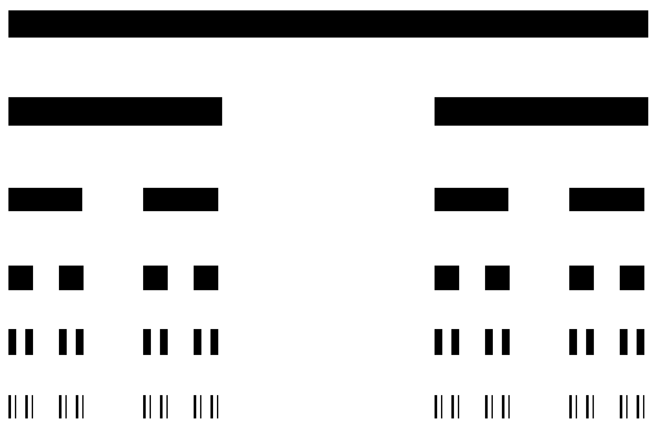
2.1. Number of Segmentations N

Assume A is a fractal object with D dimension. N is the smallest positive integer number of segmentation along ε that created the A by
N A , ε C ε D
for some positive constant C [23].

2.2. Length Estimation Using Yardstick Method

Assume f x = x 2 with 0 x 1 . We divided the f x into the several equal straight lines where ε and N ε are the length of each segmentation and the number of segmentations, respectively. The length of the curve is approximated by the multiplication of the number of segmentations N and scale ε
L = N ε · ε .
The curve is formed to the original shape, having a bigger L by using the smaller ε , so
L = lim ε 0 L ε .
Equation (3) is only applicable for the object with an irregular pattern D 1 , because the straight line’s length will be always the same for each value of ε [24].

2.3. Fractal Dimension

Let A H X where X , d is a metric space. For each ε > 0 let N A , ε denote the smallest number of closed balls of radius ε > 0 needed to cover A . If
D = lim ε 0 ln N A , ε ln 1 ε
exist, then D is called the fractal dimension of A [25].

2.4. Box-Counting Dimension

Let A H m where Euclidean metric is used. Cover m by closed square boxes of side length 1 2 n for n 1 . Let N A denote the number of boxes of side length 1 2 n which intersects the attractor A . If
D = lim n ln N A ln 2 n
exist, then D is called the fractal dimension of A [26].

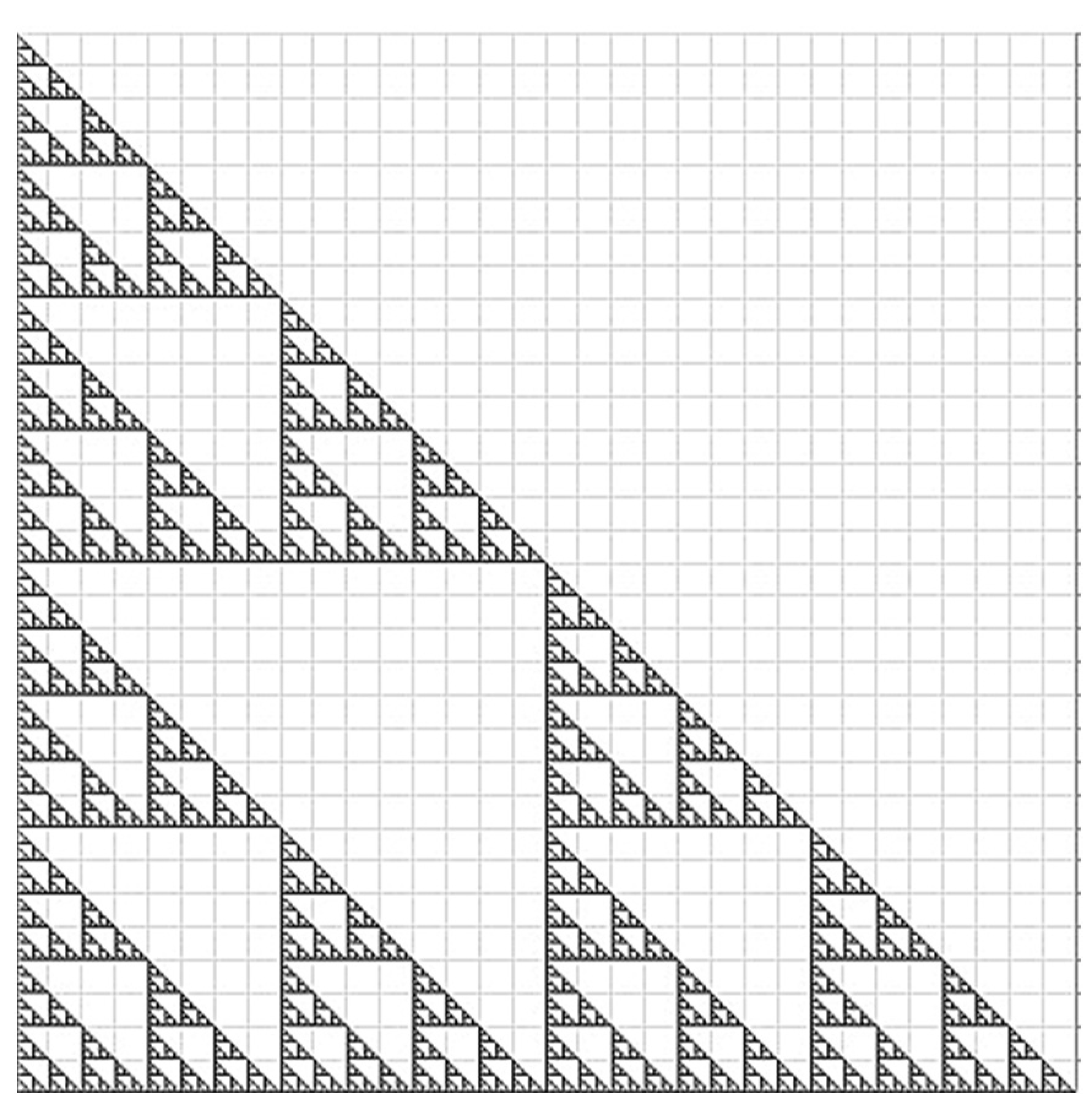
2.5. Application of Box-Counting Dimension on Sierpinski Triangle

Sierpinski Triangle is a fractal object which is created from equilateral triangles through the repeated removal of triangular subsets. Assume that there is a Sierpinski Triangle which is spanning in 0 ,   1 that has been covered by Box-Counting, as in Figure 1.
As we can see, the first triangle is divided into 3 equal triangles. Each triangle is further divided into 3 equal smaller triangles and continuously divided. By using Equation (5), we obtained the results of Table 1. From Table 1, the dimension value for each n is the same, because the triangle is subdivided recursively into smaller pieces of the bigger one [18].
The D of Figure 1 is ln 3 / ln 2 .

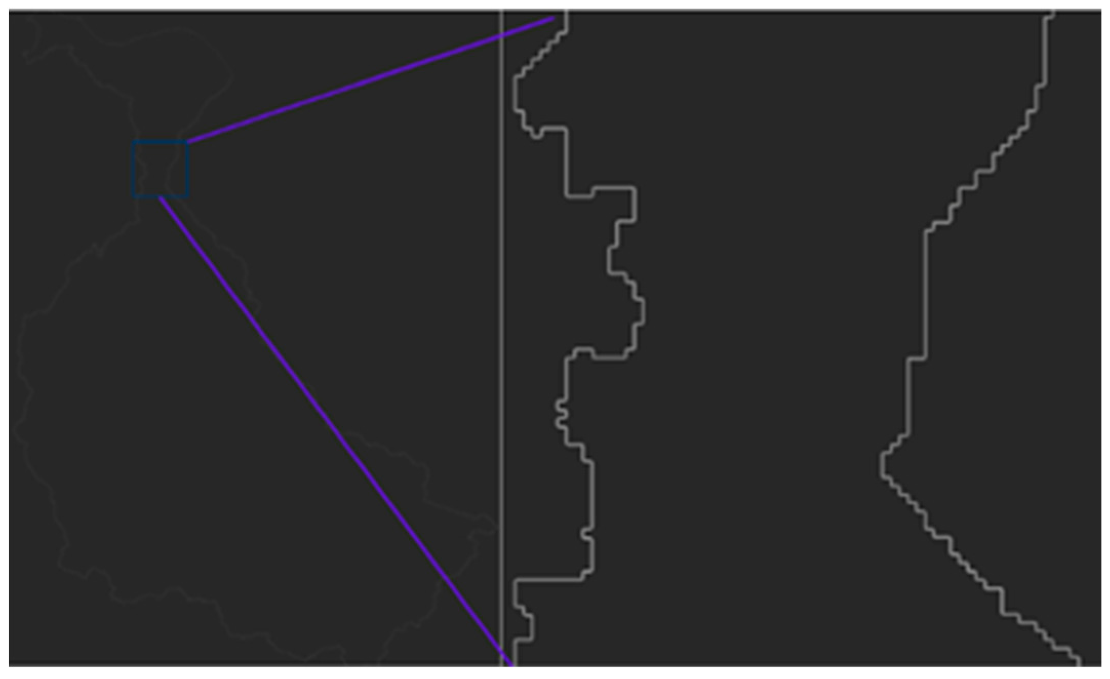
2.6. Application of Box-Counting Dimension on Irregular N

Suppose there is an object that has been applied by box-counting.
The next step is to create a graph of linear regression based on Table 2. The fractal dimension is taken from the gradient of the linear regression line, which is 1.612 [27].

2.7. Digital Image

A digital image is defined as a picture that created pixel value inside the matrix. There are 3 types of digital images, which are 3 coloring image (known as RGB image), greyscale image (known as having pixel value between 0–255), and black and white image, which is known for having a pixel value between 0 and 255 [28]. Each pixel value is represented to indicate the intensity of these three colors [29].

2.8. Edge Detection

Edge detection is defined as one of the image segmentation methods to simplify the image data to minimize the amount of processed data. By the concept, this method is the approach for meaningful discontinuities in an image [30]. The promising edge detection method is Canny edge detection, which has been used in many research and has been compared to other types of edge detection methods [31,32,33,34,35]. Based on the comparison’s result, the edge detection method that we used in this research is Canny edge detection. This method has some steps, which are:
1.
Smoothing
A process of blurring an image to reduce the noise (unused object).
2.
Finding gradients
This step aims to determine the gradient value of each pixel.
3.
Non-maximum suppression
Each pixel is compared to its neighborhood to create the edge of the first stage.
4.
Thresholding
The upper and lower threshold values are determined as the standard of the edge’s value.
5.
Edge tracking by hysteresis
Each pixel is compared to the upper and lower threshold. If the value is higher than the upper, then it is an edge. Therefore, if the value is between the upper and lower threshold but is connected to an edge, then it is an edge as well. Otherwise, the others are not the edge.
Based on the research, this step is proven to create a black and white image with thin, sharp, and detail edges compared to the other method that used different steps [36].

3. Materials and Methods

The type of this research is quantitative, which has also been included in the literature review and experimental process on simulations of fractal objects and the analytic process to calculate the length of Citarum watershed boundary. The material used for this study is a digital image of Citarum watershed boundary (see Figure 2). It has a criterion that it must be valid data from Geographics Information System (GIS), which has been proven to be generous, and a number of researchers have used these tools to calculate fractal dimension [6]. In this research, we obtained the data from the Geographics Information System by Esri (known as ArcGIS).
This research is divided into 3 main parts, which are a discussion about fractal’s power law by simulations, modification of Box-Counting’s algorithm, and calculating dimension and length estimation. The steps are described below.
1.
Literature review
The research began by collecting literature to review the Fractal theory. The relationship between the length of an object and the fractal dimension of the power law is explained by analyzing the equation.
2.
Fractal simulations
We used the equation from the previous process to explain the value of C and proved that it is equal to the previously known equation.
3.
Modification of box-counting dimension algorithm
The modification is created based on the importance of edge detection, image’s quality, thresholding process, and scale value, which can affect the results of calculation.
4.
Data processing
This step includes some processes which define the resolution of the digital image, and determine the possible value of m (the highest value of n )
5.
Canny edge detection
The purpose of this process is to create a black and white image because the data that we took from the source of GIS is an RGB image. The output is also converted into a binary pixel value.
6.
Box-Counting
This process aims to calculate the number of boxes N and determine the value of ε based on the size of box value.
7.
Calculating dimension
After we obtained the values of ε and N , we created the linear regression line and obtained the slope as the dimension of Citarum watershed Boundary.
8.
Length estimation
The values of number of boxes N , ε and D for each n , were used to calculate the length of Citarum watershed boundary. The calculation process is based on the equation in literature review and the new equation that we obtained before. This process also required converting the result from pixel units into kilometer units.

4. Modified Box-Counting Algorithm

The implementations of the box-counting dimension algorithm depend on each researcher. In this paper, we found two kinds of algorithms. The first type started by getting a high-resolution digital image from the Geographic Information System (GIS). Next, by using the image editor, the unused object was removed, leaving only the edge part. After that, the pixel matrix was processed by the box-counting application. The last step is to take the dimension by using linear regression [6]. The second type starts by finding the object and defining the pixel matrix. Then, the pixel value to the biner value is changed. After that, we determined the box-counting size and applied it to the matrix. The last part is to calculate the dimension based on the equation of slope in linear regression [38,39,40].
We modified the box-counting algorithm based on consideration of the matters mentioned above. The Box-Counting Modified Algorithm 1 is given as follows.
Algorithm 1 Modified Box-Counting Algorithm
Input. Input high-resolution image
Step 1. Execute the image by Canny Edge Detection
Step 2. Convert the black and white image into a binary value
Step 3. Find the lowest resolution on the image
Step 4. Execute box-counting
Step 5. Convert the size of the box into ε
Step 6. Create a linear regression line
Step 7. Find the slope
In Step Input, the image is obtained from geographics information system or any source which provides a high-quality image, so the result is also as accurate as possible. We used some editing features from its site/application to remove some noises from Figure 2, including the name of area, the river, lake, etc.
In Step 1, the image is executed by Canny Edge detection program. In this paper, we used Python programming language to create this program. Other programming languages can be used, as long as they can do image processing. The result of executing this program is a black and white image. The black and white image, which came as the output of Canny edge detection contains the pixel value 0 or 255.
In Step 2, each pixel value is converted to binary value, that is 0 (which is the black pixel) or 1 (which is the white pixel).
In step 3, we take the lowest resolution of the image as the m , which is the highest possible value of n .
In Step 4, through the box-counting program, execute the output of Step 2. The box sizes depend on Step 3. The result of this step is the values of the number of counted box N and the size of the box.
The process of Step 5 aims to convert the size of the box for each n from Step 4 to ε based on the length of the plane (which is 2 m + 1 ).
After we get the values of ε and N for each n , we create the linear regression line with its equation in Step 6.
The slope in Step 7 is taken from the equation of Step 6, which is the fractal dimension of the object.

5. Results

5.1. Power Law Relationship

After we showed the explanations of N and L , we substituted Equation (1) into Equation (2).
L =   N ε · ε =   C ε D · ε =   C ε 1 D
It showed that D affects the ε by the power law relationship, so it also affects the value of L . To confirm that Equation (6) is equal to Equation (2), we need to know about the value of C by doing some simulations on the fractal case.
Assume that the Cantor set exists, which spans 0 ,   3 as shown in Figure 3. Therefore, we know that the dimension of each n are the same, it is ln 2 / ln 3 . The length of iteration- n by using Equation (2) is 1 3 n 1 · 2 n . By using Equation (6), the value of C is 2 because we take the value of ε by its real length.
Let x be the length of the first line, which is 3. Then we assume that each ε means the ratio between the length of the side and x . Then the length of iteration- n by using Equation (2) is 1 3 n · 2 n · a . By using Equation (6), the value of C must be 1. In this case, we know that the value of C depends on how to define the ε . It must be 1 only and only if we define the ε as the ratio of the length of side and the length of plane, and may not be 1 if we input the real length of ε .

5.2. Experimental Results

We used the modified algorithm on the digital image of Citarum Watershed, as shown in Figure 4.
After that, we created and ran the Canny edge detection program in Figure 4, which gave the result in Figure 5.
We created the box-counting program using Python and used it to convert the pixel matrix into biner value and find the minimum resolution. This minimum resolution was used to determine the value of m , which is the highest value of n (which means that the m + 1 is the length of the plane). The criterion of m is lower than or equal to the lowest resolution. We found that the resolution of the image is 11,994 px × 16,339 px, so the minimum is 11,994 px, which means the m is 13. Based on the box-counting program, we obtained the list value of N and the converted size of the box ε shown in Table 3.
Next, the data were processed computationally to calculate the value of ln ε , ln N , and D for each n . The result is shown in Table 4.
From Table 4, the D value became smaller as ε became smaller. Based on the data we created the regression line with its equation, which is shown in Figure 6.
We found that the slope of the regression line is 1.1099, which means it is the dimension of Citarum watershed boundary, as shown in Figure 6. It is accepted because, from Table 4, the D value became smaller as ε became smaller.
We also used the data from Table 4 to estimate the length of Citarum watershed boundary. By Equation (1), the ε must be the smallest possible value, which is 2 / 2 14 . We also know that the N for that ε is 41,922, with D = 1.181186148 . By using Equation (6), the estimation of Citarum watershed boundary length is 83,884 px. Although the data that we obtained is still in pixel units, we must convert it to kilometers. We found by ARCGIS that the smallest resolution (11,994 px) stated 110.22 km, which means 1 px = 0.009189595 km. Therefore, the length of Citarum watershed boundary in kilometers is 770.49 km.

6. Discussion

Based on simulations, the new equations are obtained only and only if we define the ε as the ratio between the length of box and the length of plane, which causes the value of C = 1 . By substituting the value to Equation (1), we found
N = ε D .
We also substituted Equation (7) to Equation (6), so we found
L = ε 1 D .
The other part of this research that we can discuss is shown in Table 3. We found that the value of N became bigger while the value of ε became smaller, which makes sense, because the counted segmentation is more accurate. If we compare the D value of Citarum watershed boundary to the D value of Great Britain’s Coastline, we can conclude that the Citarum watershed boundary has a more regular shape pattern than Great Britain’s Coastline, as its value is smaller than the value that Richardson found before.

7. Conclusions

From the results, it is shown that the fractal’s power law explained the relationship between the length of an object and its dimension, proved by substituting the equations. We also created the box-counting modified algorithm based on consideration of the use of Canny edge detection and the high-resolution image. We used this algorithm to create the box-counting program, and we found that the dimension of Citarum watershed boundary was 1.1099 with a length of 770.49 km.

Author Contributions

Conceptualization, methodology, validation, M.L., H.N. and A.K.; software, M.L. and H.N.; validation, H.N. and A.K.; formal analysis, M.L. and H.N.; investigation, M.L.; resources, M.L.; writing—original draft preparation, M.L.; writing—review and editing, M.L. and H.N.; funding acquisition, H.N. and A.K. All authors have read and agreed to the published version of the manuscript.

Funding

This research was funded by Riset Percepatan Lektor Kepala (RPLK), grant number 2203/UN6.3.1/PT.00/2022.

Data Availability Statement

Not applicable.

Acknowledgments

The authors wish to thank the Directorate of Research and Community Service (DRPM) of Universitas Padjadjaran.

Conflicts of Interest

The authors declare no conflict of interest.

References

  1. Mohajeri, N.; Longley, P.; Batty, M. City Shape and the Fractality of Street Patterns. Quaest. Geogr. 2012, 31, 29–37. [Google Scholar] [CrossRef] [Green Version]
  2. Mandlebrot, B.B. The Fractal Geometry of Nature; Henry Holt and Company: New York, NY, USA, 1982. [Google Scholar]
  3. Richardson, L.F. The Problem of Contiguity: An Appendix to Statistics of Deadly Quarrels. Gen. Syst. Yearb. 1961, 6, 139–187. [Google Scholar]
  4. Mandelbrot, B. How Long Is the Coast of Britain? Statistical Self-Similarity and Fractional Dimension. Science 1967, 156, 636–638. [Google Scholar] [CrossRef] [PubMed] [Green Version]
  5. Vaughan, J.; Ostwald, M.J. Examining the Position of Wright’s Fallingwater in the Context of His Larger Body of Work: An Analysis Using Fractal Dimensions. Fractal Fract. 2022, 6, 187. [Google Scholar] [CrossRef]
  6. Husain, A.; Reddy, J.; Bisht, D.; Sajid, M. Fractal Dimension of Coastline of Australia. Sci. Rep. 2021, 11, 6304. [Google Scholar] [CrossRef]
  7. Li, C.; Xu, Y.; Jiang, Z.; Yu, B.; Xu, P. Fractal Analysis on the Mapping Relationship of Conductivity Properties in Porous Material. Fractal Fract. 2022, 6, 527. [Google Scholar] [CrossRef]
  8. Zhan, H.; Li, X.; Hu, Z.; Duan, X.; Wu, W.; Guo, W.; Lin, W. Fractal Characteristics of Deep Shales in Southern China by Small-Angle Neutron Scattering and Low-Pressure Nitrogen Adsorption. Fractal Fract. 2022, 6, 484. [Google Scholar] [CrossRef]
  9. Wen, Z.; Shen, L.; Jing, H.; Fang, K. Color and Shape Grading of Citrus Fruit Based on Machine Vision with Fractal Dimension. In Proceedings of the 2010 3rd International Congress on Image and Signal Processing, Yantai, China, 16–18 October 2010; Volume 2, pp. 898–903. [Google Scholar]
  10. Mallick, P.K.; Saravana Kumar, S.; Bhoi, A.K.; Sherpa, K.S. Brain Tumor Detection: A Comparative Analysis of Edge Detection Techniques. Int. J. Appl. Eng. Res. 2015, 10, 31569–31575. [Google Scholar]
  11. Elkington, L.; Adhikari, P.; Pradhan, P. Fractal Dimension Analysis to Detect the Progress of Cancer Using Transmission Optical Microscopy. Biophysica 2022, 2, 59–69. [Google Scholar] [CrossRef]
  12. Hu, X.; Wang, Y. Coastline Fractal Dimension of Mainland, Island, and Estuaries Using Multi-Temporal Landsat Remote Sensing Data from 1978 to 2018: A Case Study of the Pearl River Estuary Area. Remote Sens. 2020, 12, 2482. [Google Scholar] [CrossRef]
  13. Husain, A.; Reddy, J.; Bisht, D.; Sajid, M. Fractal Dimension of India Using Multicore Parallel Processing. Comput. Geosci. 2022, 159, 104989. [Google Scholar] [CrossRef]
  14. Zhu, X.; Cai, Y.; Yang, X. On Fractal Dimensions of China’s Coastlines. Math. Geol. 2004, 36, 447–461. [Google Scholar] [CrossRef]
  15. Jiang, J.; Plotnick, R.E. Fractal Analysis of the Complexity of United States Coastlines. Math. Geol. 1998, 30, 535–546. [Google Scholar] [CrossRef]
  16. Carr, J.R.; Benzer, W.B. On the Practice of Estimating Fractal Dimension. Math. Geol. 1991, 23, 945–958. [Google Scholar] [CrossRef]
  17. Bahramizadeh-sajadi, S.; Katoozian, H.R.; Mehrabbeik, M.; Baradaran-rafii, A.; Jadidi, K.; Jafari, S.; Namazi, H.; Xu, Q.; Eliasy, A. Biocybernetics and Biomedical Engineering A Fractal Approach to Nonlinear Topographical Features of Healthy and Keratoconus Corneas Pre- and Post-Operation of Intracorneal Implants. Fractal Fract. 2022, 6, 688. [Google Scholar] [CrossRef]
  18. Barnsley, M.F. Chapter V—Fractal Dimension. In Fractals Everywhere, 2nd ed.; Academic Press: Cambridge, MA, USA, 1993; pp. 171–204. ISBN 978-0-12-079061-6. [Google Scholar]
  19. Cheeseman, A.K.; Vrscay, E.R. Estimating the Fractal Dimensions of Vascular Networks and Other Branching Structures: Some Words of Caution. Mathematics 2022, 10, 839. [Google Scholar] [CrossRef]
  20. Miloevic, N.T.; Rajkovic, N.; Jelinek, H.F.; Ristanovic, D. Richardson’s Method of Segment Counting versus Box-Counting. In Proceedings of the 2013 19th International Conference on Control Systems and Computer Science, Washington, DC, USA, 29–31 May 2013; pp. 299–305. [Google Scholar]
  21. Del-Pozo-Velázquez, J.; Chamorro-Posada, P.; Aguiar-Pérez, J.M.; Pérez-Juárez, M.Á.; Casaseca-De-La-Higuera, P. Water Detection in Satellite Images Based on Fractal Dimension. Fractal Fract. 2022, 6, 657. [Google Scholar] [CrossRef]
  22. Ma, L.; He, S.; Lu, M. A Measurement of Visual Complexity for Heterogeneity in the Built Environment Based on Fractal Dimension and Its Application in Two Gardens. Fractal Fract. 2021, 5, 278. [Google Scholar] [CrossRef]
  23. Liu, S.; Chen, Y. A Three-Dimensional Box-Counting Method to Study the Fractal Characteristics of Urban Areas in Shenyang, Northeast China. Buildings 2022, 12, 299. [Google Scholar] [CrossRef]
  24. Kappraff, J. The Geometry of Coastlines: A Study in Fractals. Comput. Math. Appl. 1986, 12, 655–671. [Google Scholar] [CrossRef] [Green Version]
  25. Husain, A.; Nanda, M.N.; Chowdary, M.S.; Sajid, M. Fractals: An Eclectic Survey, Part-I. Fractal Fract. 2022, 6, 89. [Google Scholar] [CrossRef]
  26. Yu, X.; Zhao, Z. Fractal Characteristic Evolution of Coastal Settlement Land Use: A Case of Xiamen, China. Land 2022, 11, 50. [Google Scholar] [CrossRef]
  27. Jaenisch, H.M.; Potter, A.N.; Williams, D.; Handley, J.W. Fractals, Malware, and Data Models. In Proceedings of the Cyber Sensing 2012, Baltimore, MD, USA, 23–27 April 2012; Ternovskiy, I.V., Chin, P., Eds.; SPIE: Bellingham, WA, USA, 2012; Volume 8408, p. 84080X. [Google Scholar]
  28. Wevers, M.; Smits, T. The Visual Digital Turn: Using Neural Networks to Study Historical Images. Digit. Scholarsh. Humanit. 2020, 35, 194–207. [Google Scholar] [CrossRef]
  29. Arya, A.; Soni, S. Performance Evaluation of Secrete Image Steganography Techniques Using Least Significant Bit (LSB) Method. Int. J. Comput. Sci. Trends Technol. 2018, 6, 160–165. [Google Scholar]
  30. Joshi, M.; Vyas, A. Comparison of Canny Edge Detector with Sobel and Prewitt Edge Detector Using Different Image Formats. Int. J. Eng. Res. Technol. 2014, 1, 133–137. [Google Scholar]
  31. Deng, C.-X.; Wang, G.-B.; Yang, X.-R. Image Edge Detection Algorithm Based on Improved Canny Operator. In Proceedings of the 2013 International Conference on Wavelet Analysis and Pattern Recognition, Tianjin, China, 14–17 July 2013; pp. 168–172. [Google Scholar]
  32. Wang, C.; Yang, C.; Zhang, H.; Wang, S.; Yang, Z.; Fu, J.; Sun, Y. Marine-Hydraulic-Oil-Particle Contaminant Identification Study Based on OpenCV. J. Mar. Sci. Eng. 2022, 10, 1789. [Google Scholar] [CrossRef]
  33. Ma, L.; Zhang, H.; Lu, M. Building’s Fractal Dimension Trend and Its Application in Visual Complexity Map. Build. Environ. 2020, 178, 106925. [Google Scholar] [CrossRef]
  34. Shrivakshan, G.T.; Chandrasekar, C. A Comparison of Various Edge Detection Techniques Used in Image Processing. Int. J. Comput. Sci. Issues 2012, 9, 269–276. [Google Scholar]
  35. Ticala, C.; Pintea, C.M.; Matei, O. Sensitive Ant Algorithm for Edge Detection in Medical Images. Appl. Sci. 2021, 11, 11303. [Google Scholar] [CrossRef]
  36. Rana, R.; Verma, A. Comparison and Enhancement of Digital Image by Using Canny Filter and Sobel Filter. IOSR J. Comput. Eng. 2014, 16, 6–10. [Google Scholar] [CrossRef]
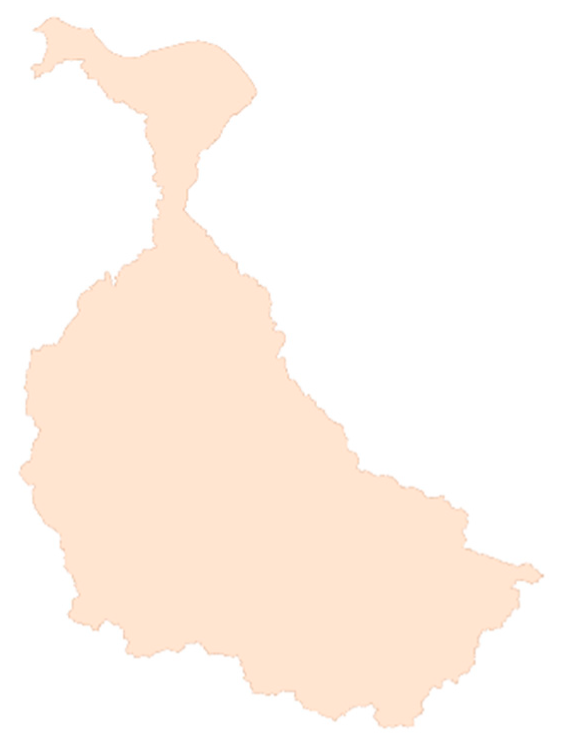
  37. Fahrizal, F. Peta Daerah Aliran Sungai Citarum. Available online: https://www.arcgis.com/home/webmap/viewer.html?webmap=41498213537843899bcbbd3ec9b6d47f (accessed on 29 November 2022).
  38. Wu, J.; Jin, X.; Mi, S.; Tang, J. An Effective Method to Compute the Box-Counting Dimension Based on the Mathematical Definition and Intervals. Results Eng. 2020, 6, 100106. [Google Scholar] [CrossRef]
  39. Koukouvelas, I.K.; Pe-Piper, G.; Piper, D.J.W. The Relationship between Length and Width of Plutons within the Crustal-Scale Cobequid Shear Zone, Northern Appalachians, Canada. Int. J. Earth Sci. 2006, 95, 963–976. [Google Scholar] [CrossRef]
  40. Hashmi, M.H.; Koloor, S.S.R.; Abdul-Hamid, M.F.; Tamin, M.N. Fractal Analysis for Fatigue Crack Growth Rate Response of Engineering Structures with Complex Geometry. Fractal Fract. 2022, 6, 635. [Google Scholar] [CrossRef]
Figure 1. Illustration of Sierpinski Triangle covered by Box-Counting [18] (modified from [18]).
Mathematics 11 00384 g001
Figure 2. Citarum River map with its watershed boundary [37].
Mathematics 11 00384 g002
Figure 3. Cantor Set.
Mathematics 11 00384 g003
Figure 4. Digital Image of Citarum Watershed [37].
Mathematics 11 00384 g004
Figure 5. Result of Canny edge detection of Figure 4.
Mathematics 11 00384 g005
Figure 6. Linear regression of Table 4.
Mathematics 11 00384 g006
Table 1. List D of Sierpinski Triangle for each n .
n N D
13 ln 2 / ln 3
29 ln 3 2 ln 2 2
327 ln 3 3 ln 2 3
m 3 m ln 3 m ln 2 m = ln 3 ln 2
Table 2. List of size and number of boxes of an irregular object.
SizeNumber of BoxesSizeNumber of Boxes
2375,200128304
497,300256119
826,07051242
167407102415
32228620484
6478940961
Table 3. Values of ε and N for each n .
ε = s i z e / 2 14 N ε = s i z e / 2 14 N
0.0001220741,9220.015625295
0.00024414121,0990.03125140
0.00048828110,5720.062563
0.00097656352810.12527
0.00195312526090.2510
0.0039062512620.53
0.0078125617
Table 4. Values of ln ε , ln N , and D for each n .
ln ε ln N D = ( ln N ) / ln 1 ε
9.01091334710.643566031.181186148
8.3177661679.9569809251.197073917
7.6246189869.2659642761.215269155
6.9314718068.5718707531.236659543
6.2383246257.8667222851.261031248
5.5451774447.1404530431.287687024
4.8520302646.4248690241.324160954
4.1588830835.6869753561.367428524
3.4657359034.9416424231.425856603
2.7725887224.1431347261.494319981
2.0794415423.2958368661.584962501
1.3862943612.3025850931.660964047
0.6931471811.0986122891.584962501
Disclaimer/Publisher’s Note: The statements, opinions and data contained in all publications are solely those of the individual author(s) and contributor(s) and not of MDPI and/or the editor(s). MDPI and/or the editor(s) disclaim responsibility for any injury to people or property resulting from any ideas, methods, instructions or products referred to in the content.

