Risk Assessment of Oil and Gas Pipeline Based on Vague Set-Weighted Set Pair Analysis Method

Abstract

This study focuses on a risk assessment method for oil and gas pipelines. Oil and gas pipelines are usually constructed in a complex geological environment and are potentially dangerous. Risk assessment is a key step for their safety management. Therefore, the present paper establishes a risk indicator system as the risk assessment foundation, and we propose a risk assessment method to obtain a quantitative assessment result for the pipeline based on set pair analysis (SPA) theory. For the weight values of each indicator in the assessment process, this paper presents a calculation method based on vague sets theory. Then, a pipeline in the Yanchang oilfield was taken as a case study to verify the feasibility of the method, and the final assessment result was 2.911, which meant the pipeline was relatively safe. The method could also obtain the risk level of each indicator, showing that geological conditions, extreme weather, and public safety awareness were particularly unsafe, and service time, pipeline deformation, ground activity, and operation training were relatively unsafe. It is expected that the risk assessment result could provide a reference for pipeline safety management.

1. Introduction

Oil and natural gas are the main energy resources used for the development of modern society, and the exploitation and transportation of oil and gas require a large number of pipelines. However, pipelines are inevitably damaged by external force, corrosion, etc., and this high risk is generated from the beginning of the pipeline’s operation. Therefore, as a piece of engineering equipment that is highly invested in, the risk management for pipelines is very important. Although some preventive measures can be used for protection during the design, construction, and operation of the pipeline’s life cycle, such measures will gradually fail with the increase in service life and cannot guarantee the long-term safety of the pipeline. Therefore, pipeline risk assessment is a scientific management technology proposed to ensure the safe operation of the pipeline in the whole life cycle. The accuracy of risk assessment results depends on the design of the assessment method.

The earliest risk assessment method came from accidents in the process of industrialization [1]. In the 1970s, nuclear power engineering began to introduce risk assessment, which eventually formed a complete risk management discipline [2]. In the late 1980s, risk management was applied to equipment safety problems in the petrochemical field, especially for the risk management of oil and gas pipelines that are prone to accidents. For pipelines, risk assessment consists of conducting periodic risk assessments on oil and gas pipelines in the operation period and constantly improving defect factors identified in the assessment results according to the standards or requirements, then finally realizing the comprehensive management of the pipeline’s safety. Therefore, the risk assessment of the pipeline is actually a task that goes hand in hand with the pipeline’s life cycle. Its purpose is to ensure that the pipeline is within the scope of risk safety and to provide corresponding improvement and maintenance decisions.

For pipeline risk assessment, the American Society of Mechanical Engineers (ASME) first began to study the risk of pressure vessels [3]. The American Petroleum Institute (API) published the API RP 580 normative standard of risk inspection technology that was formally proposed in 2002 [4], which completely defines how to plan testing technology and plan based on risk factors. Pipeline safety expert W. Kent Muhlbauer wrote the authoritative pipeline risk management book, the Pipeline Risk Management Manual, which is a summary of the theory and application of oil and gas pipeline risk assessment technology in the United States in the past decades [5]. Canada began to pay attention to the research of risk assessment technologies of pipelines in the 1990s and put forward a number of future research topics [6]. The HSC (Health and Safety Commission) of the UK developed the MISHAP software package for risk assessment and has achieved good practical results in using computer technology to carry out pipeline risk technology [7]. After years of practical applications in various countries, it has been shown that the risk assessment of oil and gas pipelines can improve the safety of their operation, greatly reduce additional economic expenditure, reduce engineering disasters and environmental damage, and even maximize returns in social benefits, economic costs, and risks [8]. For example, from 1987 to 1994, Amoco Corporation carried out regular risk assessments on its pipelines, which reduced the leakage rate from two-and-a-half times the industrial average to one-and-a-half times, and the company’s operating profit reached its highest level in 1994 [9]. A large number of practical applications show that the risk assessment management of oil and gas pipelines is necessary, and the reasonable use of risk assessment technology has obvious benefits for pipeline safety operations, maintenance decision making, ecological safety, etc. [10].

At present, the common methods used in risk assessment include the relative risk index method [11], the probability analysis method [12], the AHP (analytic hierarchy process) [13], ETA (event tree analysis) [14], the fuzzy comprehensive assessment method [15], FTA (fault tree analysis) [16], the risk matrix method [17], etc. Although these methods have been applied in risk assessment, the quantitative risk assessment of oil and gas pipelines is still relatively lacking and needs to be further studied. Because there are many risk factors affecting pipelines, including pipe properties, transmission media, the external environment, operating conditions, and management approaches, etc., the risk factors will also affect each other. Meanwhile, as long-life equipment, the pipeline needs a lot of time and money to obtain all the risk factors’ sample information. Therefore, the most commonly used risk assessment methods are not suitable for the fitting of multiple risk indicators or are unable to process the risk information of small samples. As such, the common risk assessment methods are not practical for pipeline risk assessment. At present, many practical problems have been solved by combining fuzzy theory with multi-criteria decision making, such as quality performance indicator evaluation [18], supplier selection [19], platform partner evaluation [20], etc.

In view of the current actual situation of pipeline operations, this paper constructs a risk indicator system for pipelines, calculates the indicator weight based on fuzzy theory, and combines this with the set pair analysis theory to propose a scientific quantitative risk assessment method for oil and gas pipelines. A large amount of risk indicator sample information can be obtained in a short time through the evaluation by experts [21,22], and it can solve the problem of less sample information regarding the pipeline. The set pair analysis method can realize the quantitative calculation of multiple indicators [23,24] with mathematical modeling to integrate the indicators’ information, and then effective decision making can be carried out.

Due to the large number of pipeline risk indicators, obtaining a large amount of indicator information will cost loads of time and money, which does not conform to the reality of management. The purpose of this paper is to obtain a more practical risk assessment method through mathematical modeling, which could meet the actual risk management requirements of pipeline engineering.

2. Failure Analysis and Risk Indicator System of Pipeline

Oil and gas pipelines are usually buried in the ground across a wide area and face problems caused by complex geology and a harsh natural environment. Therefore, the pipeline will inevitably be damaged by external force, corrosion, or other problems in operation. The CONCAWE (Conservation of Clean Air and Water in Europe) summarized the leakage accidents of crude oil pipelines in Western Europe from 1971–2012, involving 156 pipelines with a total length of 36,251 km, for which 274 leakage accidents occurred [25,26,27,28]. According to the leakage diameter, the accident statistics are shown in Figure 1.

The PHMSA (Pipeline and Hazardous Materials Safety Administration) of the United States conducted a statistical analysis of pipeline accidents from 1992 to 2012, including 5868 serious pipeline accidents [29]. The PHMSA divides the accident causes into seven forms: corrosion, excavation damage, misoperation, material/welding/equipment failure, natural force damage, other external force damage, and other reasons, as shown in

Table 1. Comparison of major pipeline accidents in the United States in percentage.

Failure Reason	Liquid Pipeline	Gas Transmission Pipeline	Gas Gathering Pipeline	Gas Distribution Pipeline
Corrosion	23.6	22.7	50.8	3.8
Excavation damage	18.8	17.3	6.9	37.8
Misoperation	7.9	2.5	1.5	7.7
Material/welding/equipment failure	24.1	22.6	16.2	5.4
Natural force	4.9	12.3	11.5	9.6
Other external force	1.9	5.3	3.8	11.5
Other reasons	18.8	17.3	9.2	24.2

.

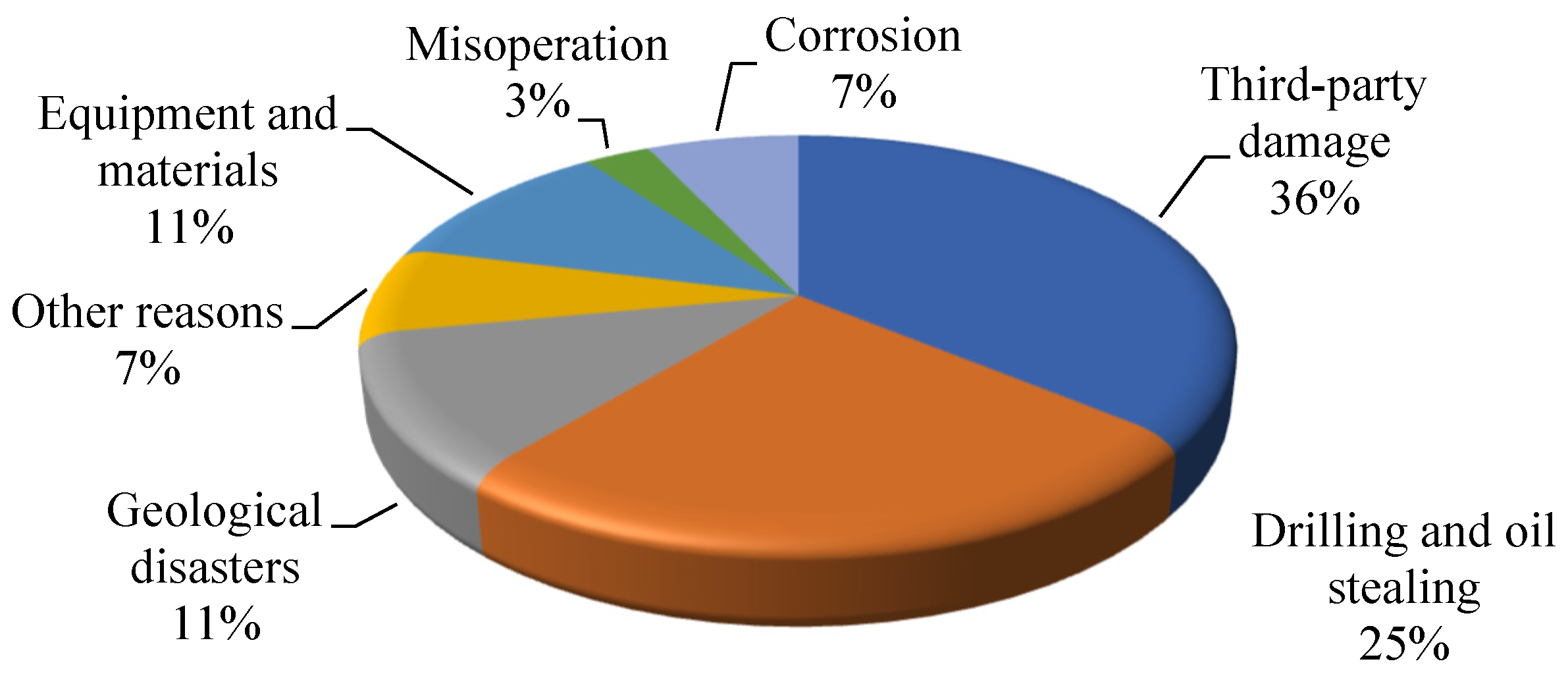
Due to the frequent production and construction activities in China, third-party damage has become an important cause of pipeline accidents, followed by corrosion. Moreover, there are more and more pipelines in complex geological areas, and pipeline accidents caused by floods, landslides, earthquakes, and other geological disasters have begun to gradually increase. There have been 28 pipeline leakage accidents in China in the past decade, as shown in Figure 2. Among them, there were 10 cases of pipeline damage caused by third-party damage, 7 cases caused by drilling and oil stealing, 3 cases caused by geological disasters, 2 cases caused by corrosion, 3 cases caused by equipment and materials, 1 case caused by improper operation, and 2 cases caused by unknown reasons.

According to the statistics of pipeline accidents in various countries, there are many causes leading to pipeline failure, including external interference, corrosion, material defects, mechanical damage, misoperation, and natural disasters. In conclusion, the analysis of the risk factors of pipelines needs to be comprehensive and save costs, so as to ensure correct and meaningful risk assessment results. The pipeline is a complex system, and the impacts of indicators on the system are different [30]. Therefore, the difficulty of obtaining indicator information is also different [31]. Therefore, the selection of indicators needs to be considered comprehensively: the obtainment of methods of indicator information should be operable, the impact on risk should be representative, and the final assessment of risk should be comprehensive. The selected indicators should be able to accurately reflect the risk status of the pipeline on a realizable basis.

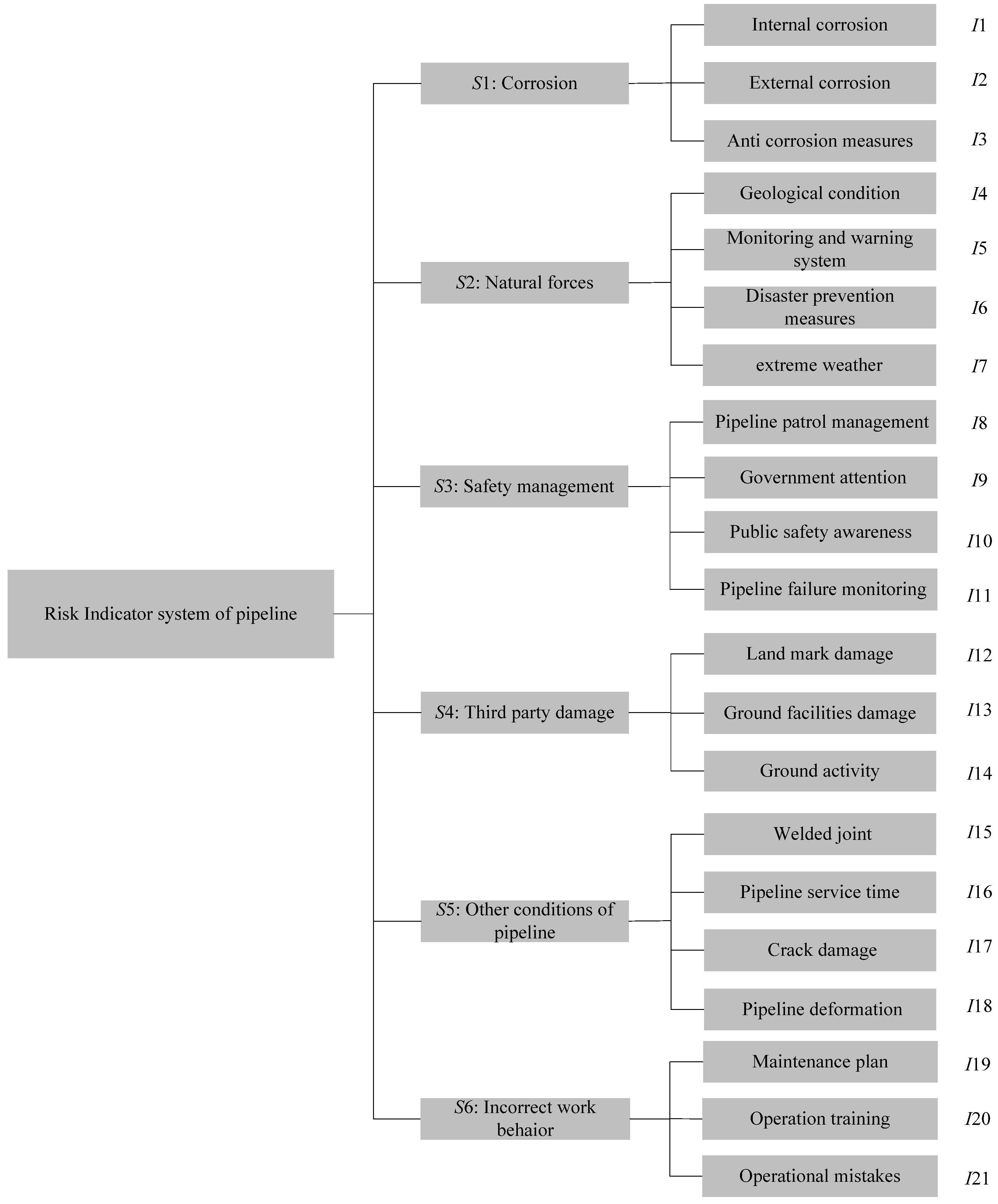
Therefore, based on the analysis of and reference to the classification of pipeline failure causes in various countries, this paper summarizes the risk indicators of pipelines into six secondary indicator sets: corrosion, third-party damage, natural forces, other conditions of the pipeline, incorrect work behavior, and safety management.

The classification of risk indicator sets is based on pipeline property damage, such as steel corrosion and cracks. Risks are caused by external factors, such as natural forces and third-party damage, as well as risks caused by incorrect operation and management, such as safety management and incorrect work behavior. Corrosion is the main form of damage to pipelines [32]. Pipeline corrosion can be divided into internal corrosion and external corrosion. External corrosion is caused by external media such as the soil and atmosphere, and internal corrosion is caused by transmission media. Natural forces are the forces of natural factors. For instance, a landslide will cause displacement and cracking of pipelines [33]. However, disasters caused by natural forces are usually sporadic and require high safety monitoring. Safety management includes the management measures taken to maintain safe operation during pipeline operation [34]. Third-party damage is the damage caused by third-party activities to pipelines [35]. For example, because of unclear ground markings, the pipeline may be exposed to the ground due to being wrongly excavated, and this will increase the risk of damage. Incorrect work behavior during pipeline operation will lead to pipeline damage. For instance, calculating the wrong delivery pressure will cause pipeline deformation. The incorrect work behavior is caused by many reasons, such as a lack of training for oil workers resulting in operational mistakes or the untimely maintenance of equipment resulting in failure. Other conditions of the pipeline include indicators that have a greater impact on pipeline safety, such as deformation, cracks, and weld joint [36].

These 6 indicator sets include 21 tertiary indicators. The final risk assessment indicator system is shown in Figure 3.

3. Set Pair Analysis Assessment Method

3.1. Set Pair Analysis Theory

Zhao [37] proposed set pair analysis method to solve the decision problem for uncertain systems, and the method is a kind of mathematical analysis theory of building correlation expression for the interaction between two different sets. The main idea of SPA is to take the certainty and uncertainty between the two sets as a system, and the certainty and uncertainty in the system are not only interrelated and interact with each other, but they are also transformed into each other under certain conditions [38]. Rong [39] used SPA and entropy theory to establish a geological disaster risk model for military engineering. Kumar [40] made each attribute and ideal attribute into a set pair to study the multi-attribute decision-making problem for an interval-valued intuitionistic fuzzy set environment. Based on SPA, Wang [41] proposed a model that considers the incompatibility, certainty, and uncertainty of assessment indicators to analyze the surrounding rock stability. Guo [42] used improved set pair analysis to calculate the relative membership degree of variable fuzzy set theory and then obtained the flood risk level for each assessment object. The mathematical expressions of set pair analysis are as follows.

(1) Assuming M and N are two sets, and defining the set pair H = (M, N), the components of M, N are shown in Figure 4, and the relational degree is defined as:

$$\mu =\frac{S}{N}+\frac{F}{N}i+\frac{P}{N}j$$

(1)

where μ is the relational degree; N is the total number of characteristics included in the set pair; and S, P, F are the common characteristic number, oppositional characteristic number, and the number of characteristics that are neither common nor oppositional of the two sets in the set pair, respectively. Without considering the weight values, S/N, F/N, and P/N are called the identity, the difference, and the opposite between the two sets, respectively, and they satisfy the constrained equation: S/N + F/N + P/N = 1, where i ∈ [0,1] is the coefficient of the difference degree, and j = −1 is the coefficient of opposition degree.

(2) Broadly speaking, any system has certainty and uncertainty information. The relational degree μ includes the certainty parts of S/N and (P/N)j and the uncertainty part of (F/N)i, and the mixture of certainty and uncertainty leads to the uncertainty of difference. Therefore, according to different backgrounds of the problem, by conducting a skewness analysis of the differences between identity and opposite, Equation (1) is expanded as:

$$\mu =\frac{S}{N}+\frac{F_1}{N}{i}_1+\frac{F_2}{N}{i}_2+\dots +\frac{F_m}{N}{i}_m+\frac{P}{N}j$$

(2)

where F₁, F₂, …, F_m are the number of characteristics that are neither included together nor opposed to each other for the two sets at different levels.

(3) Because the system usually contains multiple assessment indicators, the impact of each assessment indicator is different; therefore, it is necessary to conduct a further analysis on the identity, the difference, and the opposite of each assessment indicator in the system and to obtain the relational degree. In order to accurately reflect the influence of the assessment indicators in the system, the relational degree and the weight value of each assessment indicator should be combined to calculate the average relational degree as:

$${\mu }_a=\frac{1}{n}\cdot {\displaystyle \sum _{i=1}^n(w_n^{}\cdot {\mu }_n)}$$

(3)

where μ_a is the average relational degree, μ_n is the relational degree of indicator n, n is the number of characteristics, and w_n is the weight of μ_n.

3.2. Steps of Pipeline Risk Assessment Modeling Based on Set Pair Analysis Method

The pipeline risk assessment based on set pair analysis establishes a set pair of risk indicators and risk levels. The risk level expresses the ponderance of risk through quantitative form, for instance, to express the different risk levels through 1, 2, …, N, and the higher the number, the more serious the risk. The number of risk levels is usually set according to the actual needs of project safety management. Then, analyze the relational degree between risk indicators and the risk levels, and calculate the relational degree between each indicator and risk level. Finally, determine the eigenvalue of the pipeline risk level. The level corresponding to the eigenvalue value indicates that the risk to the pipeline has the highest relational degree with this assessment level, i.e., the risk to the pipeline belongs to the assessment level. The detailed assessment processes are as follows:

(1) Construction of set pair model for pipeline risk.

Here, the risk assessment indicators of the pipeline are determined, and the risk assessment level is established. Assume that A is the set of risk assessment indicators values, and B is the set of risk levels. The risk indicators and the risk levels are combined in pairs to establish the set pair as H(A, B):

A = {x₁, x₂, …, x_i}

(4)

$$B=\left[\begin{array}{cccc}{S}_{10}& S_{11}& \dots & S_{1j}\\ S_{20}& S_{21}& \dots & S_{2j}\\ \dots & \dots & \dots & \dots \\ S_{i0}& S_{i1}& \dots & S_{ij}\end{array}\right]$$

(5)

where x_i represents each risk indicator; S_ij is the value of the ith indicator at jth risk level.

(2) Calculating the relational degree.

According to the set pair analysis theory, the relational degree of assessment levels can be determined, and the calculation method is as follows:

$${\mu }_{ij}=\{\begin{array}{ll}1+0i_1+0i_2+0i_3+\dots +0i_{j-1}+0j\hfill & x\in [S_1,+\infty ]\hfill \\ \frac{x-S_2}{S_1-S_2}+\frac{S_1-x}{S_1-S_2}{i}_1+0i_2+0i_3+\dots +0i_{j-1}+0j\hfill & x\in [S_2,S_1]\hfill \\ 0+\frac{x-S_3}{S_2-S_3}{i}_1+\frac{S_2-x}{S_2-S_3}{i}_2+0i_3+\dots +0i_{j-1}+0j\hfill & x\in [S_3,S_2]\hfill \\ \dots \dots \hfill & \dots \dots \hfill \\ 0+0i_1+0i_2+0i_3+\dots \frac{x-S_j}{S_{j-1}-S_j}{i}_{j-1}+\frac{S_{j-1}-x}{S_{j-1}-S_j}j\hfill & x\in [S_j,S_{j-1}]\hfill \\ 0+0i_1+0i_2+0i_3+\dots +0i_{j-1}+1j\hfill & x\in [0,S_j]\hfill \end{array}$$

(6)

where x is the specific value of the risk indicator, and S₁, S₂, …, S_j−1 and S_j are the critical values of risk indicators at each assessment level. The critical values of different risk indicators at the same risk level are generally different.

3.3. Calculation Method of Risk Level

For the risk assessment level, the principle of maximum membership [43] is usually used to select the level of the maximum value in the average relation to be the final risk level. In practice, though, it is found that the influence of other relational degrees on the assessment results cannot be ignored, so the calculation method of the risk level needs to be further improved.

It is assumed that the identity, the difference, and the opposite in the average relational degree are represented as a, b₁, b₂, …, b_N−2, and c, respectively, and a, b₁, …, c ∈ [0,1], a + b₁ + b₂, …, b_n−1 + c = 1 [44].

Define the maximum value v_max as:

v_max = max{a, b₁, b₂, …, b_N−2, c}

(7)

with

v_max ≤ ∑{a, b₁, b₂, …, b_N−2, c} − v_max

(8)

Equation (8) shows that only when v_max > 0.5 can the level of v_max represent the final risk level. Therefore, this paper uses the level eigenvalue to determine the final risk level. The calculation method of the level eigenvalue is as follows:

$$S={\displaystyle \sum [a\cdot 1+b_1\cdot 2+b_2\cdot 3+\dots +b_N{}_{-2}}+c\cdot N]$$

(9)

where S is the level eigenvalue. Equation (9) shows that all values in the relational degree are considered. The range of the level eigenvalue is [1, N): 1 means the best condition without any problems, N means the worst case, and 1 and N are ideal in practice. Therefore, the risk level is identified by the level eigenvalues as follows:

level 1: e₁ ∈ [1, 1.5);

level 2: e₂ ∈ [1.5, 2.5);

......

level N−1: e_N−1 ∈ [N − 1.5, N − 0.5);

level N, e_N ∈ [N − 0.5, N].

where e_i is the eigenvalue, with conservative treatment of the upper bounds of the interval.

4. Calculation of Risk Indicator Weight Value

4.1. Analysis of Indicator Weight Calculation Method

For any risk assessment method, the weight calculation is an important component [45], and the accuracy of the weight is directly related to the accuracy of the final assessment result [46]. As a complex system, the oil and gas pipeline has multiple and closely related assessment indicators, and each indicator value has different influences on the assessment result. How to reasonably define the effect of these indicators’ values and obtain the assessment result with a high reference for a risk management decision is a key step in the assessment process.

At present, a large amount of research has been carried out on weight calculation methods, and common methods include the binomial coefficient method [47], the Delphi method [48], the Analytic Hierarchy Process (AHP) [49], etc., which are based on the knowledge and cognitive judgment of decision makers. Other methods include principal component analysis (PCA) [50], the entropy value method [51], the variation coefficient method [52], etc., which are determined according to the relationship between the indicator data and have a strong mathematical basis. The theoretical forms of these methods are different, and each has its own advantages, but it has been found that the weighting calculation methods that are most commonly used are subjective methods [53], because these are usually in line with the actual needs, and so there will be no contradiction between theory and reality, and the assessment results also usually conform to the reality and the psychological expectations. The general calculation idea is to transform the stochastic or fuzzy uncertainty into certainty under some conditions, and then carry out mathematical processing, but these uncertainties usually only describe specific situations, without considering the uncertain information that still exists in a certain range of uncertain information. However, due to the imperfection of the analysis theory, the traditional weighting methods generally neglect to simplify this uncertainty information, but with the increasing precision of engineering management and decision making, it has been found that this uncertain information really determines the final assessment result.

Therefore, in view of the fuzziness of pipeline risk indicator information, this paper applies the vague set theory to calculate the weight of the risk assessment indicator on the premise of respecting subjective experience.

4.2. Calculation Method for Risk Indicator Weight Based on Vague Set Theory

Because the cost and time of obtaining pipeline risk indicator values are different, some of them have a higher cost and take a longer time, and many indicators cannot give specific values, so the indicators’ values are generally evaluated based on an expert’s knowledge. However, experts usually cannot give specific assessment information, and the assessment information of risk indicators is usually uncertain. In this paper, the assessment information of indicators is expressed in the form of a vague value. The vague value considers the negative effects of uncertainty, and the uncertainty information can be analyzed accurately [54]. This method has been widely used in the field of decision management [55], so this paper uses vague set theory to design indicator weights, and the basic theory of vague sets is shown in Appendix A. The calculation steps are as follows.

(1) The vague value of the indicator be constructed by expert assessment, and the assessment matrix for risk is described by Equation (10):

$$C=\left(\begin{array}{ccccc}{c}_{11}& c_{12}& c_{13}& \dots & c_{1m}\\ c_{21}& c_{22}& c_{23}& \dots & c_{2m}\\ \dots & \dots & \dots & \dots & \dots \\ c_{n1}& c_{n2}& c_{n3}& \dots & c_{nm}\end{array}\right)$$

(10)

where c_nm = [t_nm,1 − f_nm] is the vague value of the indicator.

(2) The consistency matrix is represented as [56]:

$$M^k=\left(\begin{array}{ccccc}{M}_{11}^k& M_{12}^k& M_{13}^k& \dots & M_{1n}^k\\ M_{21}^k& M_{22}^k& M_{23}^k& \dots & M_{2n}^k\\ \dots & \dots & \dots & \dots & \dots \\ M_{n1}^k& M_{n2}^k& M_{n3}^k& \dots & M_{nn}^k\end{array}\right)$$

(11)

with

$$M_{xy}=1-\frac{\left|t_x-t_y-(f_x-f_y)\right|}{2}$$

(12)

where $M_{ij}^k$ is the similarity value between vague values evaluated by different experts. x = [t(x),1 − f(x)] and y = [t(y),1 − f(y)] are vague values. Therefore, M^k is the measure of the similarity of all the experts’ assessments of the indicator. If the similarity value is closer to 1, the experts have more consistent opinions, and if the similarity value is closer to 0, the experts’ opinions are inconsistent. The average similarity value for the indicator is represented by

$$V_i^k=\frac{1}{n}{\displaystyle \sum _{j=1}^n{M}_{ij}^k}$$

(13)

(3) The relative consistency values of each expert to every index are mathematically represented by

$$d_{ik}=\frac{V_i^k}{{\displaystyle \sum _{i=1}^n{V}_i^k}}$$

(14)

Therefore, the relative consistency measure matrix of indexes evaluated by experts is represented by

$$D=\left(\begin{array}{ccccc}{d}_{11}& d_{12}& d_{13}& \dots & d_{1m}\\ d_{21}& d_{22}& d_{23}& \dots & d_{2m}\\ \dots & \dots & \dots & \dots & \dots \\ d_{n1}& d_{n2}& d_{n3}& \dots & d_{nm}\end{array}\right)$$

(15)

where D can be interpreted as the information representation of each expert’s preference.

(4) The indicators of the preference information for all the experts are defined by [57]:

$$c_k={\displaystyle \sum _{i=1}^{n}D\otimes c_{ik}}=\left[{\displaystyle \sum _{i=1}^n{d}_{ik}{t}_{ik}},1-{\displaystyle \sum _{i=1}^n{d}_{ik}{f}_{ik}}\right]$$

(16)

where c_k is the assessment vague value of all experts. Finally, according to c_k, the weight is defined as [58]

$$w_s^k=t_k+(1-t_k-f_k)/2$$

(17)

where $w_s^k$ is the subjective weight and includes two parts: agreement and uncertainty. For the uncertainty, this paper defines half of it as agreement and the other half as disapproval. t_k is the truth membership degree of the vague value, where f_k is the false membership degree of the vague value, where t_k and f_k are represented in Equations (18) and (19):

$$t_k={\displaystyle \sum _{i=1}^n{d}_{ik}{t}_{ik}}$$

(18)

$$f_k={\displaystyle \sum _{i=1}^n{d}_{ik}{f}_{ik}}$$

(19)

5. A Case Study

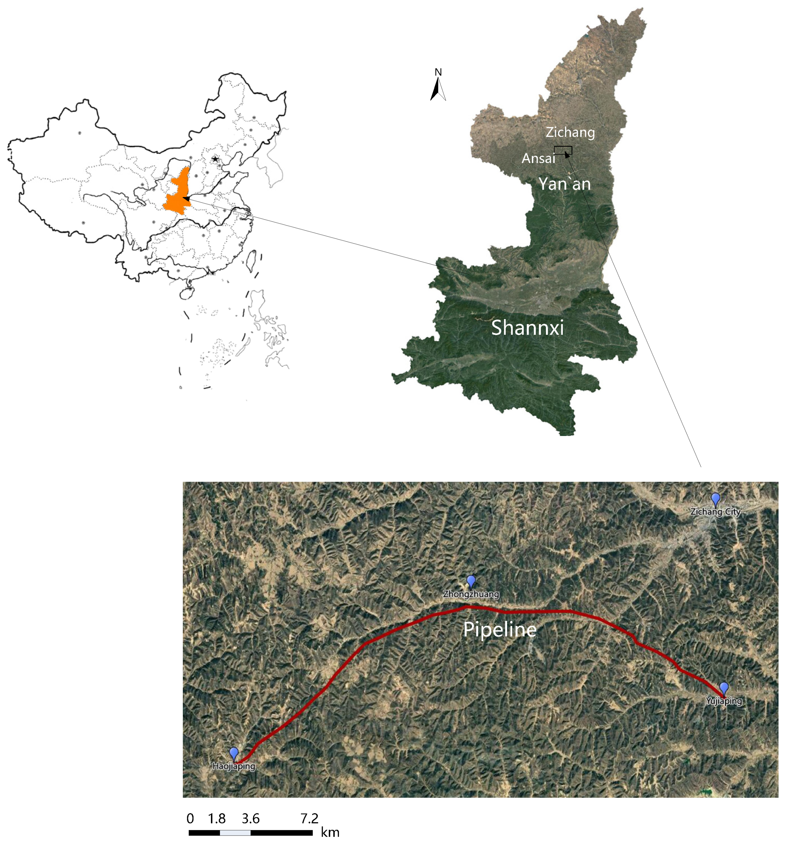
The Yujiaping-Haojiaping pipeline belongs to the Yanchang oilfield and stretches from the Xingzichuan oil production plant to the Yongping oil refinery, located in Yan’an City, Shaanxi Province, China (Figure 5). The basic pipeline information is shown in

Table 2. Basic information on pipeline.

Parameter	Values
Total length	36.0 km
Service time	12a
Pipe diameter	219 mm
Pipe type	Seamless pipe
Pipeline steel	X42
Pipe wall thickness	6.4 mm
Specified Minimum Yield Strength (SMYS)	290 MPa (GB/T9711)
Maximum allowable operating pressure (MAOP)	3.8 MPa
Design operating pressure	4 MPa
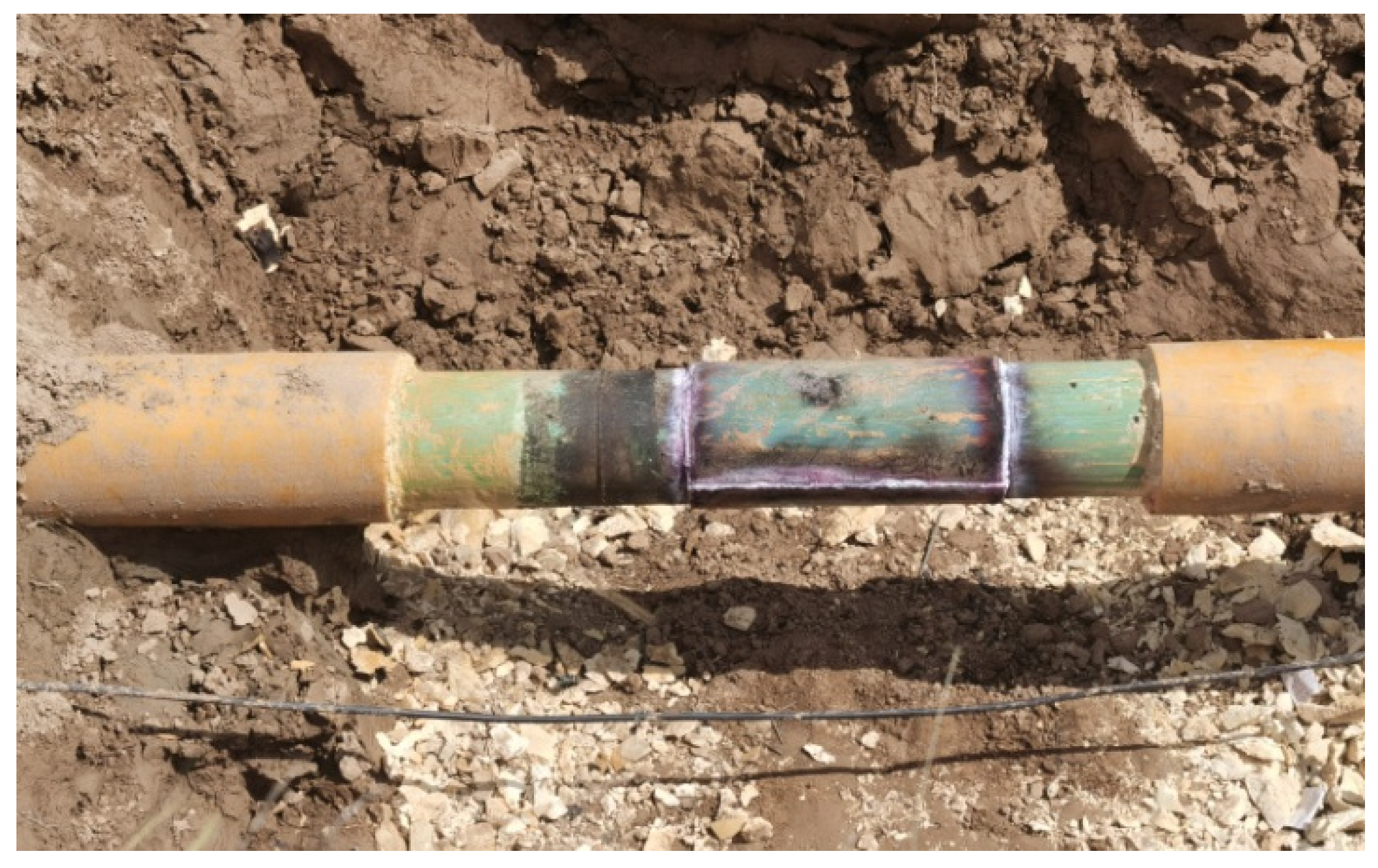
Medium transported	Crude oil and gas

. The pipeline has been in operation for more than ten years, and it began to gradually form sudden damage. The sudden damage, such as leakage, seriously affects the normal transportation of oil and brings pressure to pipeline maintenance. (Figure 6) Therefore, for the purpose of providing a reference to make maintenance decisions in advance, a risk assessment is now carried out for this pipeline.

5.1. Calculation of Risk Indicator Weight

The accurate assessment method must be based on the appropriate assessment information. The assessment information usually includes the assessment indicators and the assessment standard. The assessment indicators are listed in the Section 2. For the assessment standard, the more the assessment levels there are, the more accurate the final assessment result will be. However, too many assessment levels will lead to complexity in the calculation in the assessment process, and it will also lead to complexity in the expression of the results from the qualitative assessment point of view. The psychologist George Miller [59] proved that the number of levels for which a human can correctly distinguish things is between five and nine, and based on national standards [60,61]. This paper divides the safety of pipeline into 5 assessment levels: L₁ is extremely safe; L₂ is very safe; L₃ is relatively safe; L₄ is relatively unsafe; L₅ is particularly unsafe (can be understood as failure), and the score ranges are (0.9,1), (0.8,0.9), (0.7,0.8), (0.6,0.7), (0,0.6), respectively. The five assessment levels can reasonably reflect the different states of pipeline risk from serious to safe. L₁ and L₅ represent the most extreme state, and L₁ means that all the pipeline indicators are perfect without any need of improvement. L₅ means that the pipeline has great risks, cannot be operated, and needs maintenance. L₃ represents a stable safety state. In L₃, although there are some defect indicators, they do not affect the operation of the pipeline, and the defect indicators only need to be monitored regularly. L₂ is a safer state than L₃. Some defect indicators have been improved in L₂, but there are still a few defect indicators that cannot be further improved. L₄ indicates that at this time, the pipeline has some risk problems that need to be corrected. Although these problems will not affect the normal operation of the pipeline temporarily, they will further increase the risk of pipeline failure in the short term.

The assessment of indicators is also divided into six levels, and the vague values are constructed: V₁ (0.9,1), V₂ (0.8,0.9), V₃ (0.6,0.8), V₄ (0.4,0.6), V₅ (0.2,0.3), V₆ (0,0.2). Eight experts in pipeline safety management are invited to judge the indicators and give the vague values.

Taking the corrosion indicator as an example, the magnetic flux leakage detector (Figure 7) is used to detect the corrosion data. The internal corrosion situation and external corrosion situation of the pipeline are shown in Figure 8, and experts can give the vague value based on this corrosion information.

The vague value of other indicators can also be given by expert judgement based on the testing or recording data. Natural force indicators can be judged based on the recorded data of natural resource departments and meteorological departments. Safety management indicators, third-party damage indicators, and incorrect work behavior indicators can be judged based on the recorded data of the pipeline operation department. Other conditions of pipeline indicators can be judged based on the equipment detection data. The assessment vague values are given based on the six levels shown in

Table 3. Vague value of indicators.

Indicator	Vague Value
Internal corrosion	[0.8,0.9]	[0.9,1]	[0.8,0.9]	[0.6,0.8]	[0.9,1]	[0.6,0.8]	[0.8,0.9]	[0.9,1]
External corrosion	[0.8,0.9]	[0.8,0.9]	[0.8,0.9]	[0.9,1]	[0.9,1]	[0.9,1]	[0.8,0.9]	[0.8,0.9]
Anti-corrosion measures	[0.9,1]	[0.9,1]	[0.9,1]	[0.8,0.9]	[0.9,1]	[0.8,0.9]	[0.6,0.8]	[0.4,0.6]
Geological condition	[0.4,0.6]	[0.2,0.3]	[0.2,0.3]	[0.2,0.3]	[0.2,0.3]	[0.4,0.6]	[0.1,0.2]	[0.8,0.9]
Monitoring and warning system	[0.8,0.9]	[0.9,1]	[0.9,1]	[0.6,0.8]	[0.8,0.9]	[0.8,0.9]	[0.9,1]	[0.6,0.8]
Disaster prevention measures	[0.8,0.9]	[0.8,0.9]	[0.9,1]	[0.9,1]	[0.9,1]	[0.9,1]	[0.9,1]	[0.6,0.8]
Extreme weather	[0.4,0.6]	[0.4,0.6]	[0.2,0.3]	[0.6,0.8]	[0.2,0.3]	[0.4,0.6]	[0.2,0.3]	[0.1,0.2]
Pipeline patrol management	[0.8,0.9]	[0.8,0.9]	[0.6,0.8]	[0.6,0.8]	[0.8,0.9]	[0.6,0.8]	[0.6,0.8]	[0.6,0.8]
Government attention	[0.8,0.9]	[0.9,1]	[0.9,1]	[0.9,1]	[0.9,1]	[0.9,1]	[0.9,1]	[0.8,0.9]
Public safety awareness	[0.1,0.2]	[0.2,0.3]	[0.4,0.6]	[0.2,0.3]	[0.2,0.3]	[0.1,0.2]	[0.2,0.3]	[0.8,0.9]
Pipeline failure monitoring	[0.6,0.8]	[0.8,0.9]	[0.6,0.8]	[0.8,0.9]	[0.8,0.9]	[0.6,0.8]	[0.8,0.9]	[0.8,0.9]
Landmark damage	[0.6,0.8]	[0.8,0.9]	[0.8,0.9]	[0.6,0.8]	[0.8,0.9]	[0.8,0.9]	[0.9,1]	[0.8,0.9]
Ground facilities’ damage	[0.8,0.9]	[0.8,0.9]	[0.8,0.9]	[0.9,1]	[0.8,0.9]	[0.8,0.9]	[0.8,0.9]	[0.1,0.2]
Ground activity	[0.6,0.8]	[0.8,0.9]	[0.6,0.8]	[0.8,0.9]	[0.4,0.6]	[0.6,0.8]	[0.8,0.9]	[0.6,0.8]
Welded joint	[0.8,0.9]	[0.9,1]	[0.9,1]	[0.6,0.8]	[0.9,1]	[0.8,0.9]	[0.6,0.8]	[0.8,0.9]
Service time	[0.6,0.8]	[0.9,1]	[0.4,0.6]	[0.1,0.2]	[0.8,0.9]	[0.6,0.8]	[0.1,0.2]	[0.9,1]
Crack damage	[0.9,1]	[0.8,0.9]	[0.8,0.9]	[0.6,0.8]	[0.9,1]	[0.9,1]	[0.6,0.8]	[0.6,0.8]
Pipeline deformation	[0.4,0.6]	[0.4,0.6]	[0.6,0.8]	[0.8,0.9]	[0.2,0.3]	[0.2,0.3]	[0.8,0.9]	[0.8,0.9]
Maintenance plan	[0.8,0.9]	[0.8,0.9]	[0.6,0.8]	[0.6,0.8]	[0.8,0.9]	[0.8,0.9]	[0.6,0.8]	[0.6,0.8]
Operation training	[0.8,0.9]	[0.6,0.8]	[0.8,0.9]	[0.1,0.2]	[0.8,0.9]	[0.6,0.8]	[0.1,0.2]	[0.4,0.6]
Operational mistakes	[0.6,0.8]	[0.8,0.9]	[0.9,1]	[0.9,1]	[0.8,0.9]	[0.6,0.8]	[0.8,0.9]	[0.9,1]

.

Based on vague values and Equation (10), the risk assessment matrix is:

$$C=\left(\begin{array}{ccccc}[0.8,0.9]& [0.9,1]& [0.8,0.9]& \dots & [0.9,1]\\ [0.8,0.9]& [0.8,0.9]& [0.8,0.9]& \dots & [0.8,0.9]\\ \dots & \dots & \dots & \dots & \dots \\ [0.6,0.8]& [0.8,0.9]& [0.9,1]& \dots & [0.9,1]\end{array}\right)$$

Taking the first indicator of internal corrosion as an example, the consistency matrix is calculated by Equations (11) and (12):

$$M^1=\left(\begin{array}{ccccc}1& 0.9& 1& \dots & 0.9\\ 0.9& 1& 0.9& \dots & 1\\ \dots & \dots & \dots & \dots & \dots \\ 0.9& 1& 0.9& \dots & 1\end{array}\right)$$

where ${\displaystyle \sum _{j=1}^8{M}_{1j}^1=7.4}$, and the average similarity value of each expert can be calculated by Equation (13):

$$V_i^1 = [7.4, 7.2, 7.4, 6.8, 7.2, 6.8, 7.4, 7.3]$$

and ${\displaystyle \sum _{i=1,j=1}^8{M}_{ij}^1=57.4}$, so we can obtain the relative consistency value of each expert on internal corrosion:

$$d_{ik} = V_i^1/57.4 = [0.1289, 0.1254, 0.1289, 0.1185, 0.1254, 0.1185, 0.1289, 0.1272]$$

Furthermore, the relative consistency measure matrix of indicators evaluated by experts is represented by:

$$D=\left(\begin{array}{ccccc}0.1289& 0.1262& \dots & \dots & 0.1185\\ 0.1254& 0.1262& \dots & \dots & 0.1289\\ \dots & \dots & \dots & \dots & \dots \\ 0.1272& 0.1262& \dots & \dots & 0.1271\end{array}\right)$$

The assessment vague value of all experts on internal corrosion in can be obtained:

$$\begin{array}{c}{t}_1={\displaystyle \sum _{i=1}^n{d}_{i1}{t}_{i1}}=0.1289\times 0.8+0.1254\times 0.9+\dots +0.1272\times 0.9=0.7918\\ f_1={\displaystyle \sum _{i=1}^n{d}_{i1}{f}_{i1}}=0.1289\times (1-0.9)+0.1254\times (1-1)+\mathrm{...0.1271}\times (1-1)=0.0861\end{array}$$

Finally, the weight of internal corrosion is:

$$w_s^1=0.7918+(1-0.7918-0.0861)/2=0.8528$$

The weights of each indicator are calculated respectively, and the results are shown in the

Table 4. Indicator weight.

Indicator	Weight	Indicator	Weight
Internal corrosion	0.055258	Landmark damage	0.053573
External corrosion	0.057462	Ground facilities’ damage	0.053004
Anti-corrosion measures	0.055084	Ground activity	0.047607
Geological condition	0.023032	Welded joint	0.055267
Monitoring and warning system	0.055201	Service time	0.042459
Disaster prevention measures	0.058215	Crack damage	0.053911
Extreme weather	0.024772	Pipeline deformation	0.039098
Pipeline patrol management	0.048906	Maintenance plan	0.050213
Government attention	0.060031	Operation training	0.040487
Public safety awareness	0.019645	Operational mistakes	0.055258
Pipeline failure monitoring	0.051519	-	-

.

5.2. Establishment of Set Pair Analysis for Pipeline Risk

The risk level and the indicator set are constituted as a set pair. The indicators corresponding to levels L₁ to L₅ are respectively defined as the identity, the difference trend to identity, the difference, the difference trend to opposite, and the opposite, and the number of indicators is S, F₁, F₂, F₃, and P, respectively. The calculation steps of the five-element relational degree for the pipeline are as follows.

(1) Because the safety of the pipeline is divided into five assessment levels, the five-element relational degree according to the risk assessment level can be assessed with:

$${\mu }_a=\frac{S}{N}+\frac{F_1}{N}{i}_1+\frac{F_2}{N}{i}_2+\frac{F_3}{N}{i}_3+\frac{P}{N}j$$

(20)

(2) The relation degree of each indicator is calculated based on the median value of each vague value. The calculation method is:

$${\mu }_{ij}=\{\begin{array}{cc}1+0i_1+0i_2+0i_3+0j& x\in [1,+\infty ]\\ \frac{x-0.9}{1-0.9}+\frac{1-x}{1-0.9}{i}_1+0i_2+0i_3+0j& x\in [0.9,1]\\ 0+\frac{x-0.8}{0.9-0.8}{i}_1+\frac{0.9-x}{0.9-0.8}{i}_2+0i_3+0j& x\in [0.8,0.9]\\ 0+0i_1+\frac{x-0.7}{0.8-0.7}{i}_2+\frac{0.8-x}{0.8-0.7}{i}_3+0j& x\in [0.7,0.8]\\ 0+0i_1+0i_2+\frac{x-0.6}{0.7-0.6}{i}_3+\frac{0.7-x}{0.7-0.6}j& x\in [0.6,0.7]\\ 0+0i_1+0i_2+0i_3+1j& x\in [0,0.6]\end{array}$$

(21)

where x is the median value of the vague value. Taking internal corrosion as an example, the median values of the vague value given by experts are (0.85, 0.95, 0.85, 0.7, 0.95, 0.7, 0.85, 0.95). The relational degrees of all experts calculated based on Equation (21) are shown in the

Table 5. Relational degrees of internal corrosion.

	1	i1	i2	i3	j
1	0	0.5	0.5	0	0
2	0.5	0.5	0	0	0
3	0	0.5	0.5	0	0
4	0	0	0	1	0
5	0.5	0.5	0	0	0
6	0	0	0	1	0
7	0	0.5	0.5	0	0
8	0.5	0.5	0	0	0
average	0.1875	0.375	0.1875	0.25	0

.

Combining the indicator weight 0.55258 (in Table 4), the comprehensive relational degree of internal corrosion is calculated as:

$${\mu }_a^1 = 0.0104 + 0.0207i_1 + 0.0104i_2 + 0.0138i_3 + 0j$$

5.3. Calculate the Relational Degree and Determine the Risk Level

By calculating the relational degree of all risk indicators, the five-element average relational degree of pipeline risk is calculated as:

μ_a = 0.1288 + 0.3167i₁ + 0.1983i₂ + 0.2271i₃ + 0.1291j

Because the max value in {S, F₁, F₂, F₃, P} is less than 0.5, the principle of maximum membership cannot be used to determine the final risk level. Therefore, the risk level eigenvalue value is calculated based on Equation (9):

S = 0.1288 × 1 + 0.3167 × 2 + 0.1983 × 3 + 0.2271 × 4 + 0.1291 × 5 = 2.911

The risk level eigenvalue of the pipeline is calculated as 2.911, i.e., the risk level is L₃, which means the pipeline is relatively safe. This also indicates that the risk level of the pipeline is at L₃ but tends to L₂, that is, it is could attain level L₂ through improvement. The relational degree and level eigenvalues of the six indicator sets can be calculated as shown in

Table 6. Relational degree and level eigenvalues of indicator set.

Indicator Set	1	i1	i2	i3	j	Eigenvalue
Corrosion	0.2080	0.4178	0.2098	0.1234	0.0410	2.3716
Natural forces	0.1770	0.2739	0.1611	0.1285	0.2594	3.0195
Safety management	0.1250	0.3138	0.1888	0.2770	0.0954	2.9041
Third-party damage	0.0432	0.3386	0.2954	0.2412	0.0816	2.9794
Incorrect work behavior	0.0710	0.2800	0.2090	0.3360	0.1040	3.1221
Other conditions of pipeline	0.1352	0.2772	0.1420	0.2597	0.1860	3.0842

. Meanwhile, the assessment result also indicates that some indicators are not perfect. The calculation results of the risk level eigenvalue for each indicator are shown in

Table 7. Risk eigenvalues of indicator.

Indicator Set	Indicator	Eigenvalue	Indicator	Indicator Set	Eigenvalue
Corrosion	Internal corrosion	2.5000	Third-party damage	Landmark damage	2.7500
	External corrosion	2.1250		Ground facilities’ damage	2.6875
	Anti-corrosion measures	2.5000		Ground activity	3.5625
Natural forces	Geological conditions	4.6875	Safety management	Pipeline patrol management	3.4375
	Monitoring and warning system	2.5000		Government attention	1.7500
	Disaster prevention measures	2.0625		Public safety awareness	4.6875
	Extreme weather	4.8750		Pipeline failure monitoring	3.0625
Other conditions of pipeline	Welded joint	2.5000	Incorrect work behavior	Maintenance plan	3.2500
	Service time	3.5625		Operation training	3.8125
	Crack damage	2.6875		Operational mistakes	2.5000
	Pipeline deformation	3.9375		-	-

.

5.4. Analysis of Assessment Results

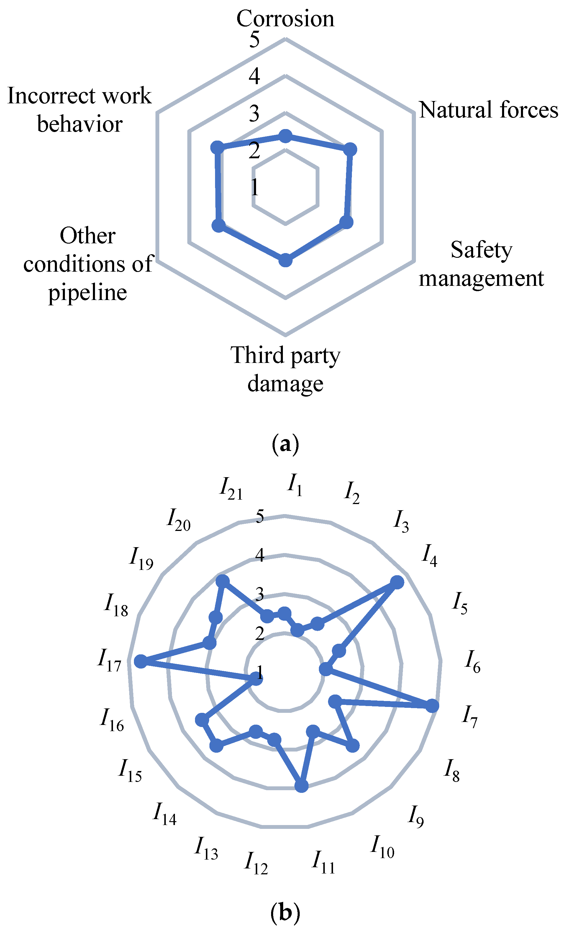
The risk eigenvalues of the indicator sets and indicators are shown in Figure 9. Figure 9a shows that the corrosion is at the L₂ level (i.e., very safe), and the natural forces, incorrect work behavior, third-party damage, and other conditions of pipeline are at the L₃ level (i.e., relatively safe).

Figure 9b shows that geological conditions, extreme weather, and public safety awareness are at the L₅ level (i.e., particularly unsafe), and service time, pipeline deformation, ground activity, and operation training are at the L₄ level (i.e., relatively unsafe). These indicators have an obvious influence on the safety of pipeline. Among these indicators, geological conditions, extreme weather, and service time are indicators that cannot be changed or modified from the perspective of management and can only be prevented in the form of periodic detection. Pipeline deformation needs to be focused on and monitored in time, and timely maintenance is necessary. However, public safety awareness, ground activity, and operation training awareness can be corrected and improved in a timely manner. By improving the three indicators, the safety of the pipeline can be greatly improved.

Other indicators affecting the risk are in line with the safety regulations and within the acceptable range of safety. However, with the increase in the pipeline’s operation time, the insecurity of these indicators will increase, and this will affect the overall safety. Therefore, targeted monitoring should be carried out according to the different risk levels. In particular, it is necessary point out that the impact of the risk of misoperation on the safety of the pipeline is controllable, which requires more strict control.

6. Conclusions

In this paper, set pair analysis theory is used to assess pipeline risk. Vague set theory is applied to calculate the weights of the identity, the difference, and the opposite. The calculation method takes into account the subjective influence of experts’ preferences and improves the accuracy and reasonableness of the assignment of weights. Meanwhile, to solve the problem that the risk level judgement with the maximum membership method is usually inconsistent with the actual situation, this paper uses the eigenvalue method to calculate the risk level and considers the influence of other relational degrees on the final result.

The risk indicators of pipelines are various and complex. In many cases, these indicators have a comprehensive effect and promote or inhibit to each other. Meanwhile, because the risk indicators are too numerous and studying all of them to obtain greater detailed information will take a lot of money and time, this is not suitable for actual engineering issues. Compared with traditional risk assessment methods, this paper proposes a new weight calculation method for the uncertainty of pipeline risk assessment indicators. Compared with other fuzzy expressions (e.g., fuzzy numbers), the vague value can express fuzzy information and comprehensively characterize the indicator information. It solves the uncertainty and hesitation of experts in judging risk indicators and renders the pipeline risk indicator weight calculation method more scientific. Compared with the traditional multi-criteria judgement method, the set pair analysis method connects the assessment indicators with the assessment criteria and can scientifically and quantitatively calculate the comprehensive judgment result of a large amount of indicator information. The assessment decision-making method proposed in this paper is to calculate the relational degree between indicators with all assessment levels, and this is reflected in the final assessment results. Other decision-making methods, for example, the TOPSIS method in [18], included calculating the relationship between indicators with the best and worst assessment levels, which cannot reflect the membership degree to other risk assessment levels, and this will then lead to a certain error in the final evaluation results. Therefore, the assessment results in this paper are more comprehensive, stable, and accurate. The method proposed in this paper solves the problem of quantitative risk assessment for pipelines in the absence of indicator information and is more suitable for the situation in which there are only a small amount of sample data in the risk assessment.

Meanwhile, the assessment method proposed in this paper uses the multi-index assessment of pipeline risk for a single objective decision. The method not only realizes the quantification of risk assessment, but it also accurately reflects the comprehensive risk level for the pipeline and provides a new idea for the safety management of the pipeline. At the same time, the method can also locate the deficiencies of specific indicators, which is helpful for managers to make targeted improvements. The method has good practicability and is conducive to the long-term operation and management of pipelines, and it also provides a reference for other engineering projects’ risk assessments. However, the method relies too much on the experience, knowledge base, and judgement ability of experts, so it has a personal preference effect on the assessment results and does not exclusively use the indicators’ information. Therefore, it is necessary to further study the ways in which to combine the existing indicator information to form a more comprehensive assessment method.

References

1. Holland, M.L. Cost saving achievable through application of risk based inspection Philosophies. In Risk, Economy and Safety Failure, Minimisation and Analysis; Penny, R.K., Ed.; CRC Press: Boca Raton, FL, USA, 1998; pp. 28–35. [Google Scholar]
2. US NRC. WASH-1400: Reactor safety study: An Assessment of Accident Risks in U.S. In Commercial Nuclear Power Plants; US NRC: Rockville, MD, USA, 1975. [Google Scholar]
3. Phillips, J.H. Reliability and risk in pressure vessels and piping. In Proceedings of the 1993 Pressure Vessels and Piping Conference, Denver, CO, USA, 25–29 July 1993; pp. 25–29. [Google Scholar]
4. API 580-2002; Risk-Based Inspection Recommend Practice. American Petroleum Institute: Washington, WA, USA, 2002.
5. Muhlbauer, W.K. Pipeline Risk Management Manual, 2nd ed.; Gulf Publishing Company: Houston, TX, USA, 1992. [Google Scholar]
6. Feng, X.D.; Zhang, S.Z.; Wang, R.J. Study on safety management system of oil and gas pipeline in Canada and its implications. J. Saf. Sci. Technol. 2016, 6, 180–186. (In Chinese) [Google Scholar]
7. Bilo, M.; Kinsman, P. MISHAP-HSE’s pipeline risk-assessment methodology. Pipes Pipelines Int. 1997, 42, 5–12. [Google Scholar]
8. Zhao, Z.G.; Yao, A.L.; Zhao, X.F. Research progress in risk assessment of oil and gas pipeline acceptability. Technol. Superv. Pet. Ind. 2005, 21, 94–98. (In Chinese) [Google Scholar]
9. Huang, W.H. The application actualities of foreign pipeline risk management and the future work for China to do. Oil Gas Storage Transporation 2001, 20, 1–10. (In Chinese) [Google Scholar]
10. Arzaghi, E.; Abbassi, R.; Garaniya, V.; Binns, J.; Khan, F. An ecological risk assessment model for Arctic oil spills from a subsea pipeline. Mar. Pollut. Bull. 2018, 135, 1117–1127. [Google Scholar] [CrossRef]
11. Zhang, H.L.; Feng, Y.J.; Zhang, C.H. Application of Risk Index Method in Pipeline Construction. Pet. Eng. Constr. 2012, 38, 1–4. (In Chinese) [Google Scholar]
12. Mustaffa, Z. Developments in Reliability-Based Assessment of Corrosion. In Developments in Corrosion Protection; Aliofkhazraei, M., Ed.; IntechOpen Limited: London, UK, 2014; pp. 681–698. [Google Scholar]
13. Yasseri, S.F.; Mahani, R.B. Pipeline Risk Assessment Using Analytic Hierarchy Process (AHP). In Proceedings of the ASME 30th International Conference on Ocean, Offshore and Arctic Engineering, Rotterdam, The Netherlands, 19–24 June 2011; pp. 1–11. [Google Scholar]
14. Hong, E.S.; Lee, I.M.; Shin, H.S.; Nam, S.W.; Kong, J.S. Quantitative risk assessment based on event tree analysis technique: Application to the design of shield TBM. Tunn. Undergr. Space Tech. 2009, 24, 269–277. [Google Scholar] [CrossRef]
15. Fan, C.G.; Dou, F.S.; Tong, B.M.; Long, Z.Q. Risk Analysis Based on AHP and Fuzzy Comprehensive Assessment for Maglev Train Bogie. Math. Probl. Eng. 2016, 2016, 1–10. [Google Scholar]
16. Shahriar, A.; Sadiq, R.; Tesfamariam, S. Risk analysis for oil & gas pipelines: A sustainability assessment approach using fuzzy based bow-tie analysis. J. Loss Prevent. Proc. 2012, 25, 505–523. [Google Scholar]
17. Lu, L.L.; Liang, W.; Zhang, L.B.; Zhang, H.; Lu, Z.; Shan, J.Z. A comprehensive risk assessment method for natural gas pipelines by combining a risk matrix with a bow-tie model. J. Nat. Gas Sci. Eng. 2015, 25, 124–133. [Google Scholar] [CrossRef]
18. Snežana, N.; Ranka, G.; Tijana, P. Quality Performance Indicators Evaluation and Ranking by Using TOPSIS with the Interval-Intuitionistic Fuzzy Sets in Project-Oriented Manufacturing Companies. Mathematics 2022, 10, 4174. [Google Scholar]
19. Wang, C.N.; Nguyen, V.T.; Kao, J.C. Multi-Criteria Decision-Making Methods in Fuzzy Decision Problems: A Case Study in the Frozen Shrimp Industry. Symmetry 2021, 13, 370. [Google Scholar] [CrossRef]
20. Bao, Y.G.; Zhang, X.Y.; Zhou, T.T.; Chen, Z.H. Application of Industrial Internet for Equipment Asset Management in Social Digitalization Platform Based on System Engineering Using Fuzzy DEMATEL-TOPSIS. Machines 2022, 10, 1137. [Google Scholar] [CrossRef]
21. Katarina, R.; Jelena, K.P.; Nikša, J. Knowledge-Based Fuzzy Expert System to the Condition Assessment of Historic Road Bridges. Appl. Sci. 2021, 11, 1021. [Google Scholar]
22. Peng, S.H.; Tang, C. Blending the Analytic Hierarchy Process and Fuzzy Logical Systems in Scenic Beauty Assessment of Check Dams in Streams. Water 2015, 7, 6983–6998. [Google Scholar] [CrossRef] [Green Version]
23. Xie, D.L.; Han, J.; Zhang, H.D.; Wang, K. Risk Assessment of Water Inrush from Coal Seam Roof Based on Combination Weighting-Set Pair Analysis. Sustainability 2022, 14, 11978. [Google Scholar] [CrossRef]
24. Wang, R.; Zhao, Q.; Sun, H.; Zhang, X.D. Risk Assessment Model Based on Set Pair Analysis Applied to Airport Bird Strikes. Sustainability 2022, 14, 12877. [Google Scholar] [CrossRef]
25. Schäfer, H.; Bottari, A. Performance of European Cross Country Oil Pipelines Detailed Description of Reported Spillages 1971–1983; CONCAWE Oil Pipelines Management Group’s Special Task Force on Oil Pipeline Spillages: Brussels, Belgium, 1985. [Google Scholar]
26. Schäfer, H.; Bottari, A. Performance of European Cross Country Oil Pipelines Detailed Description of Reported Spillages 1984–1993; CONCAWE Oil Pipelines Management Group’s Special Task Force on Oil Pipeline Spillages: Brussels, Belgium, 1994. [Google Scholar]
27. Davis, P.M.; Giessler, K.P. Performance of European Cross Country Oil Pipelines Detailed Description of Reported Spillages 1994–2004; CONCAWE Oil Pipelines Management Group’s Special Task Force on Oil Pipeline Spillages: Brussels, Belgium, 2006. [Google Scholar]
28. Schäfer, H.; Diaz, J.M. Performance of European Cross Country Oil Pipelines Detailed description of reported spillages 2005–2012; CONCAWE Oil Pipelines Management Group’s Special Task Force on Oil Pipeline Spillages: Brussels, Belgium, 2013. [Google Scholar]
29. Pipeline Incidents and Mileage Reports. Available online: http://primis.phmsa.dot.gov/comm/reports/safety/PSI.html?nocache=8699 (accessed on 2 March 2013).
30. Ding, P. Research on Safety Reliability and Risk Assessment of Submarine Pipeline. Ph.D. Thesis, School of Petroleum Engineering, China University of Petroleum (East China), Beijing, China, 2008. [Google Scholar]
31. Brito, A.J.; Almeida, A.T.D. Multi-attribute risk assessment for risk ranking of natural gas pipelines. Reliab. Eng. Syst. Safe 2009, 94, 187–198. [Google Scholar] [CrossRef]
32. Kim, S.J.; Choe, B.H.; Kim, W. A fuzzy inference based reliability method for underground gas pipelines in the presence of corrosion defects. J. Korean Inst. Intell. Syst. 2016, 26, 343–350. [Google Scholar] [CrossRef]
33. Alvarado-Franco, J.P.; Castro, D.; Estrada, N.; Caicedo, B. Quantitative-mechanistic model for assessing landslide probability and pipeline failure probability due to landslide. Eng. Geol. 2017, 222, 212–224. [Google Scholar] [CrossRef]
34. Adegboye, M.A.; Fung, W.K.; Karnik, A. Recent Advances in Pipeline Monitoring and Oil Leakage Detection Technologies: Principles and Approaches. Sensors 2019, 19, 2548. [Google Scholar] [CrossRef] [Green Version]
35. Xiang, W.; Zhou, W. Bayesian network model for predicting probability of third-party damage to underground pipelines and learning model parameters from incomplete datasets. Reliab. Eng. Syst. Safe 2021, 205, 107262. [Google Scholar] [CrossRef]
36. Dmytrakh, I.M.; Leshchak, R.L.; Syrotyuk, A.M.; Barna, R.A. Effect of hydrogen concentration on fatigue crack growth behaviour in pipeline steel. Int. J. Hydrog. Energ. 2017, 42, 6401–6408. [Google Scholar] [CrossRef]
37. Zhao, K.Q. An applications of the scheme-appraisal decision matrix based on set pair analysis. Syst. Eng. 1994, 12, 67–72. (In Chinese) [Google Scholar]
38. Zhao, K.Q.; Xuan, A.L. Set pair theory-a new theory method of non-define and its applications. Syst. Eng. 1996, 14, 18–23. (In Chinese) [Google Scholar]
39. Rong, Q.B. Entropy-Based Set Pair Analysis Model on Geological Disaster Risk for Military Engineering. Engineering 2012, 4, 76–82. [Google Scholar] [CrossRef] [Green Version]
40. Kumar, K.; Garg, H. TOPSIS method based on the connection number of set pair analysis under interval-valued intuitionistic fuzzy set environment. Comput. Appl. Math. 2018, 37, 1319–1329. [Google Scholar] [CrossRef]
41. Wang, M.W.; Xu, X.Y.; Li, J.; Jin, J.L. A Novel Model of Set Pair Analysis Coupled with Extenics for Assessment of Surrounding Rock Stability. Math. Probl. Eng. 2015, 2015, 1–9. [Google Scholar]
42. Guo, E.L.; Zhang, J.Q.; Ren, X.H.; Zhang, Q. Integrated risk assessment of flood disaster based on improved set pair analysis and the variable fuzzy set theory in central Liaoning Province, China. Nat. Hazards 2014, 74, 947–965. [Google Scholar] [CrossRef]
43. Wang, J.Q.; Zhou, L. Grey random multi-criteria decision-making approach based on maximum membership degree. Control Decis. 2010, 25, 493–501. (In Chinese) [Google Scholar]
44. Zhao, K.Q. Decision making algorithm based on set pair analysis for use when facing multiple uncertain attributes. CAAI Trans. Intell. Syst. 2010, 5, 41–50. (In Chinese) [Google Scholar]
45. Peng, Z.L.; Zhang, Q.; Yang, S.L. Overview of comprehensive assessment theory and methodology. Chin. J. Manag. Sci. 2015, 23, 245–256. (In Chinese) [Google Scholar]
46. Pang, Y.J.; Liu, K.D.; Zhang, B.W. The method of determining the objective index weight in the synthetic assessment system. System Eng. Theor. Prac. 2001, 21, 37–42. [Google Scholar]
47. Cheng, M.X. The method of weighted sum of binomial coefficients for multi-objective decision making. System Eng. Theor. Prac. 1983, 4, 23–26. [Google Scholar]
48. Shands, F.; Levary, R.R. Weighting the importance of various teacher behaviors by use of the delphi method. Education 1986, 106, 306–320. [Google Scholar]
49. Shen, R.; Meng, X.; Yu, Y. Analytic hierarchy process applied to synthetically evaluate the labour intensity of jobs. Ergonmics 1990, 33, 867–874. [Google Scholar] [CrossRef]
50. Prado, B.Q.D.M.; Fernandes, H.R.; Araújo, T.G.; Laia, G.A.; Biase, N.G. Assessment of climatological variables in Uberlandia (MG) by principal component analysis. Eng. Sanit Ambient. 1990, 21, 407–413. [Google Scholar] [CrossRef] [Green Version]
51. Gorgij, A.D.; Kisi, O.; Moghaddam, A.A.; Taghipour, A. Groundwater quality ranking for drinking purposes, using the entropy method and the spatial autocorrelation index. Environ. Earth Sci. 2017, 76, 261–269. [Google Scholar] [CrossRef]
52. Zheng, H.P.; Xue, M.; Han, Y.; Zhang, W.C. Application of the variation coefficient method to comprehensive assessment of wind farms. Appl. Mech. Mater. 2014, 488, 1447–1453. [Google Scholar] [CrossRef]
53. Liu, Q.Y.; Wu, X.N. Review on the Weighting Methods of Indexes in the Multi-Factor Assessment. Knowl. Manag. Forum 2017, 8, 500–510. (In Chinese) [Google Scholar]
54. Zhang, Q.H.; Xiao, Y.; Wang, G.Y. A new method for measuring fuzziness of vague set (or intuitionistic fuzzy set). J. Intell. Fuzzy Syst. 2013, 25, 505–515. [Google Scholar] [CrossRef]
55. Wang, J.; Xu, W.; Ma, J.; Wang, S.Y. A vague set based decision support approach for evaluating research funding programs. Eur. J. Oper. Res. 2013, 230, 656–665. [Google Scholar] [CrossRef]
56. Yi, X.; Zhang, F.L.; Qiu, H. Optimization of construction project group based on combination of vague set and IAHP. Stat. Decis. 2013, 29, 34–37. (In Chinese) [Google Scholar]
57. Liu, A.H.; Shi, S.L.; Wu, C. The synthetic assessment for systematic safety based on Vague sets. Eng. Sci. 2007, 9, 58–61. [Google Scholar]
58. Zhou, H.Y.; Wen, L.P. A new approach of group decision making under vague preference. Math. Pract. Theory 2004, 34, 6–11. (In Chinese) [Google Scholar]
59. Miller, G.A. The magical number seven, plus or minus two: Some limits on our capacity for processing information. Psychol. Rev. 1956, 63, 81–97. [Google Scholar] [CrossRef] [Green Version]
60. Chen, Y.N.; Xie, S.Y.; Tian, Z.G. Risk assessment of buried gas pipelines based on improved cloud-variable weight theory. Reliab. Eng. Syst. Safe 2022, 221, 108374. [Google Scholar] [CrossRef]
61. Ba, Z.N.; Wang, Y.; Fu, J.S.; Liang, J.W. Corrosion Risk Assessment Model of Gas Pipeline Based on Improved AHP and Its Engineering Application. Arab J. Sci. Eng. 2022, 47, 10961–10979. [Google Scholar] [CrossRef]
62. Gau, W.L.; Buehrer, D.J. Vague sets. IEEE Trans. Syst. Man Cybern. 1993, 23, 610–614. [Google Scholar] [CrossRef]
63. Zeng, W.Y.; Zhao, Y.B.; Gu, Y.D. Similarity measure for vague sets based on implication functions. Knowl. Based Syst. 2016, 94, 124–131. [Google Scholar] [CrossRef]
Figure 1. Statistical chart of leakage accidents.
Mathematics 11 00349 g001
Figure 2. Statistics of pipeline leakage accidents in China.
Mathematics 11 00349 g002
Figure 3. Risk failure indicator system of oil and gas pipeline.
Mathematics 11 00349 g003
Figure 4. Schematic diagram of internal relationship between each component of the set pair analysis relational degree.
Mathematics 11 00349 g004
Figure 5. Location of the studied pipeline.
Mathematics 11 00349 g005
Figure 6. Pipeline maintenance.
Mathematics 11 00349 g006
Figure 7. Magnetic flux leakage detector.
Mathematics 11 00349 g007
Figure 8. Axial distribution of corrosion in pipeline: (a) axial distribution of internal corrosion in pipeline; (b) axial distribution of external corrosion in pipeline. The yellow and green lines indicate E.R.F values under different corrosion damages. E.R.F is an estimated maintenance factor, which is the basis for judging whether maintenance is required and the severity of corrosion damage.
Mathematics 11 00349 g008
Figure 9. Risk eigenvalues of the indicator sets and indicators: (a) risk eigenvalues of the 6 indicator sets; (b) risk eigenvalues of all the indicators.
Mathematics 11 00349 g009