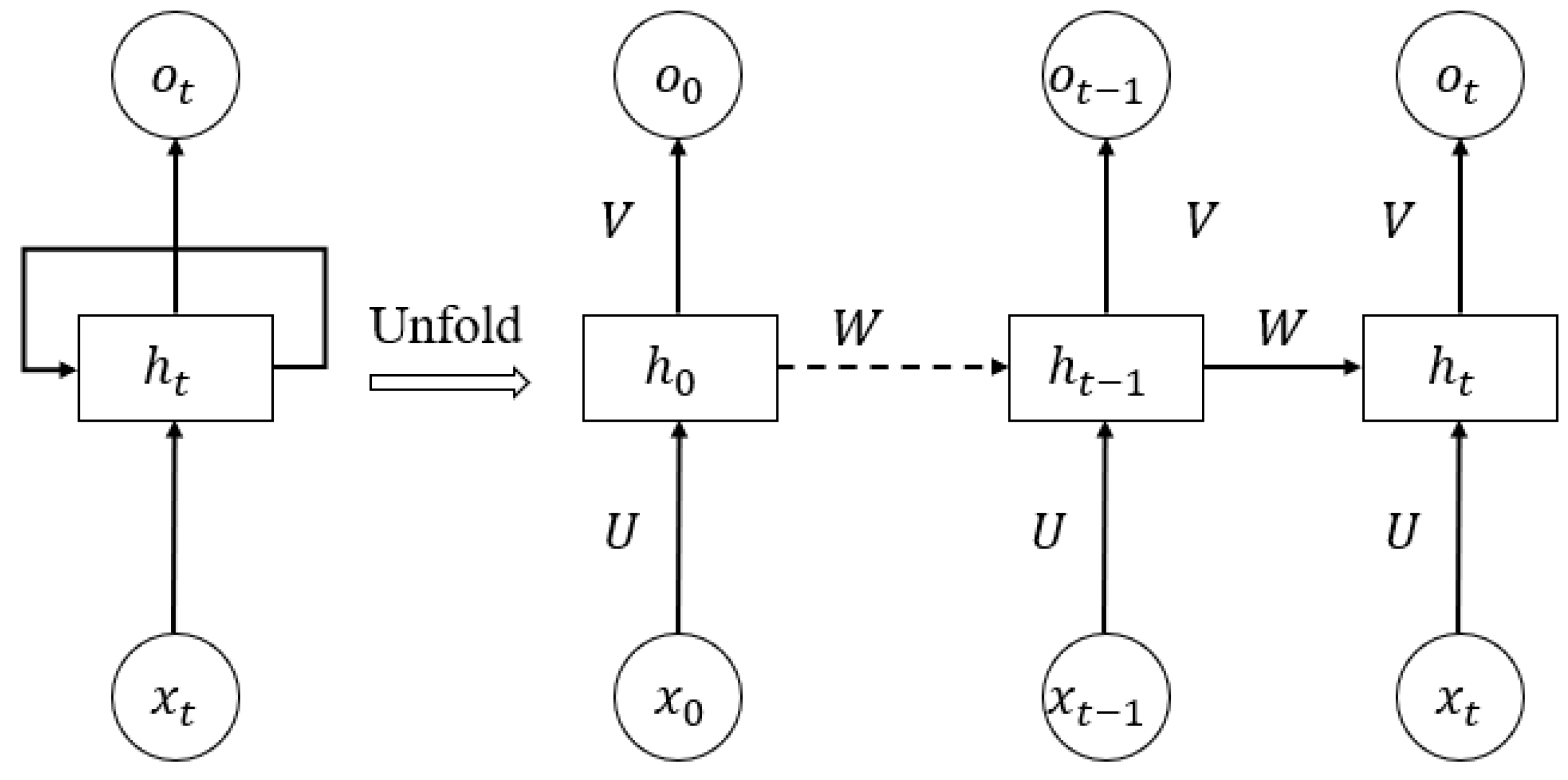
Article

Option Pricing Using LSTM: A Perspective of Realized Skewness

School of Economics, Ocean University of China, Qingdao 266100, China
*
Author to whom correspondence should be addressed.
Mathematics 2023, 11(2), 314; https://doi.org/10.3390/math11020314
Submission received: 21 December 2022 / Revised: 2 January 2023 / Accepted: 5 January 2023 / Published: 7 January 2023
(This article belongs to the Special Issue Advanced Research in Mathematical Economics and Financial Modelling)

Abstract

:
Deep learning has drawn great attention in the financial field due to its powerful ability in nonlinear fitting, especially in the studies of asset pricing. In this paper, we proposed a long short-term memory option pricing model with realized skewness by fully considering the asymmetry of asset return in emerging markets. It was applied to price the ETF50 options of China. In order to emphasize the improvement of this model, a comparison with a parametric method, such as Black-Scholes (BS), and machine learning methods, such as support vector machine (SVM), random forests and recurrent neural network (RNN), was conducted. Moreover, we also took the characteristic of heavy tail into consideration and studied the effect of realized kurtosis on pricing to prove the robustness of the skewness. The empirical results indicate that realized skewness significantly improves the pricing performance of LSTM among moneyness states except for in-the-money call options. Specifically, the LSTM model with realized skewness outperforms the classical method and other machine learning methods in all metrics.
MSC:
91G20; 68T07

1. Introduction

As a momentous derivative financial instrument, the option plays a crucial role in risk management and price discovery. The rapid development of the modern options market is attributed to the great breakthrough published by Black, Scholes, and Merton [1,2,3]. Thereafter, option pricing has become a hot topic in the derivative financial market.
As the most famous parametric method for option pricing, the Black-Scholes (BS) formula is put forward based on five assumptions, among which the most controversial ones are the constant volatility and log normality of the underlying asset return. To overcome the drawbacks of the BS formula, many improvements have been worked out to contribute to this field. For example, against the assumption of constant volatility, Heston introduced a stochastic volatility option pricing model [4]. Duan [5] assumed that the volatility of the underlying asset return followed a GARCH process. With the development of data processing capability, realized vpolatility, which is a non-parametric volatility measurement based on high-frequency data, has also been incorporated into the BS pricing framework [6,7,8].
For the normal assumption, the evidence has been established that the distribution of asset returns in financial market is asymmetric, especially for emerging financial market [9,10,11]. The characteristic of heavy tail of financial asset return cannot be ignored either [12]. Therefore, some researchers applied skewness for option pricing to get an analytic option pricing formula, achieving more accurate pricing performance [13,14,15]. Since the Edgeworth expansion has a significant advantage in characterizing the non-normality distribution of underlying assets [16], Duan et al. [17,18] developed a general analytical approximation method for pricing European options based on an Edgeworth series expansion for adjusting skewness and kurtosis of the cumulative asset return in the framework of GARCH.
Another branch of option pricing studies focuses on non-parametric methods, such as machine learning. Neural network, Support vector machine (SVM), Random forests, Extreme gradient boosting (XGBoost), and Light Gradient Boosting Machine (LightGMB) have achieved empirical success in predicting financial asset price [19,20,21,22,23,24,25,26]. However, financial data presents feature of high frequency and serial correlation. Due to the great ability in non-linear fitting and time-series information extraction, a variety of deep-learning methods have already been applied to predict financial asset price, such as long short-term memory (LSTM) model [27,28,29,30]. Zhang and Huang [31] applied the long short-term memory recurrent neural network (LSTM-RNN) for hedging. The deep-learning neural network has also been proven efficient for option pricing [32,33,34,35,36]. For example, attempts have been made to use deep-learning models on American options [37,38]. Nevertheless, these methods only focus on refining the structure of the neural network itself, ignoring the stylized facts of financial asset return, especially the skewness.
In light of the above information, an LSTM neural network [39] with realized skewness was proposed. The feasibility of implementing this model in option pricing is tested with the ETF50 options of China. Realized volatility, strike price, maturity, risk-free interest rate, and underlying asset price, which are usually deployed for derivatives pricing, and realized skewness, the one considered in our study, have been adopted as our input features. Furthermore, realized kurtosis has also been considered as one of the input features when testing the robustness of realized skewness. In comparison to the model without realized skewness and the model that contains realized skewness and realized kurtosis, our algorithm containing only realized skewness was applicable to acquire the intraday price and shows better pricing performance. Moreover, to verify the performance of the LSTM model when considering realized skewness, benchmark models were exercised for pricing options [40,41,42,43,44,45]. Several evaluating metrics, such as mean square error (MSE), root mean square error (RMSE), mean absolute error (MAE) and mean absolute percentage error (MAPE), were used to test the pricing accuracy of our proposed model.
The remainder of this paper is organized as follows. Section 2 provides a brief background of the LSTM neural network and recurrent neural network (RNN) and gives the model structure adopted in this paper. Section 3 conducts an empirical study for pricing ETF50 options and model comparison. Section 4 provides some concluding remarks.

2. Methodology

2.1. Recurrent Neural Network

The recurrent neural network, which is one of the most popular deep-learning algorithms, is a variant structure of an artificial neural network. It is usually used for processing time-sequential data due to its ability to capture the relationship between previous period data and current data. The output features of the previous period are retained during the training process and are computed as input variables for the next period. The result of the computation of the t − 1 period of the hidden state will be considered as the input variable for period t and multiplied by a weight. Then, the activation function maps the hidden state to the output state. The neurons of each layer are illustrated in Figure 1, where x t is an input vector at time-step t, h t is the hidden state vector at time-step t, o t is the output at time-step t, W is the weight from the hidden layer at time-step t − 1 to the hidden layer at time-step t, U is the weight from the input layer to the hidden layer, and V is the weight from the hidden layer to the output. The mathematical form of an RNN is given by the following formulas:
h t = f h ( U x t + W h t 1 )
o t = f o ( V h t )
where f h and f o are the activation function. In this paper, ‘ReLU’ function was applied to describe nonlinear transformation. The use of ‘ReLU’ allows the network to introduce sparsity on its own, which can greatly increase the training speed.
For this study, an RNN is proposed that is composed of five simple RNN-layers and one dense layer. Additionally, there are some dropout-layers included.

2.2. Long Short-Term Memory Neural Network

The LSTM introduced by Hochreiter and Schmidhuber uses a structure called an LSTM cell to obtain better memory. Meanwhile, in order to avoid gradient explosion and gradient extinction performed in an RNN, the LSTM uses a gate control mechanism and memory cells to control information transmission, which greatly enhances the long-term memory performance [46]. The gate control mechanism consists of an input gate i t , forget gate f t , and output gate o t , as shown in Figure 2. The input gate determines the input variable during the current period and the hidden neuron of the previous period to the memory status of the current period. The forget gate determines the portion to be forgotten from the input memory cell of the previous period to the memory status of the current period. The output gate determines the output information from the memory status. Therefore, the LSTM is specifically designed to learn long-term dependencies.
The Equations (3)–(8) portray the update of the memory cells of the LSTM. The notations of each equation are presented below:
x t is the input vector.
W f , W i , W C , and W o are the weight matrices of gate and cell states.
b f , b i , b C , and b o are bias vectors.
h t is the hidden state of the LSTM.
f t , i t , and o t are values of forget gate, input gate, and output gate, respectively.
C t is the vector for the cell states and C t ˜ is the temporary vector for the cell states.
f ( · ) is the activation function.
f t = f ( W f · [ h t 1 ,   x t ] + b f )
i t = f ( W i · [ h t 1 ,   x t ] + b i )
C t ˜ = f ( W C · [ h t 1 ,   x t ] + b C )
C t = C t 1 · f t + i t · C t ˜
o t = f ( W o · [ h t 1 ,   x t ] + b o )
h t = o t · f ( C t )
The structure of the LSTM is composed of an input layer, one or more hidden layers, and an output layer. In addition, the number of neurons in each layer is variant when considering different problems. Figure 3 shows the network architecture. When processing an input sequence, the cell states and hidden states are passed through the neurons to obtain the output. During the training process, the network updates the weights and bias terms in such a way that it minimizes the loss of the objective function over the entire training data set, whose MSE is used in this paper. In Figure 3, I n are the input features of our model. h n represents the hidden neurons of hidden layers. It only shows one hidden layer in Figure 3. O is the output of the network, and in our study, it represents the option price. The weights of each connection are adjusted according to the feedback error. In order to construct a pricing model, each layer of the LSTM is stacked with a set of neurons, as shown in Figure 2. With different amounts of neurons and different number of layers, the LSTM presents different structures and adapts to different problems. The specified topology of the LSTM model used in our study is shown in Section 2.3.

2.3. Model Structure

We construct LSTM networks containing five LSTM layers and four Dropout layers, which are used in our study for pricing the ETF50 options. The Dropout layer can prevent overfitting. With respect to the numerous factors that affect the prices of options, we consider the traditional factors that have been approved using the BS model and the realized skewness and realized kurtosis features proposed in this paper. Then, features that include spot price, strike price, risk-free rate, time-to-maturity, realized volatility, realized skewness, and realized kurtosis are selected as input variables. The structure of the LSTM used in our study is shown in Figure 4. The neural network is trained to retain the prices of the ETF50 options. Then, the predicted option prices acquired from the network and the real option prices should be compared to measure the accuracy of the network.
In the benchmarks, the structure of the RNN is shown in Figure 5. The overall number of layers of the LSTM and RNN models are equal, and the hyperparameters of each model are shown in Table 1.
Herein, [200, 200, 200, 200, 200, 1] represents the number of neurons from the first network layer to the last network layer.

2.4. Computing Realized Higher Moments

We define the intraday log-returns for each interval, and the definition of the ith log return on day t is given using
r t ,   i = 100 ( log p t , i log p t , i 1 ) i = 1 ,   2 N
where p t , i is the closing price of ETF50 on day t in ith interval. We use one-minute intraday price so that we have N = 241 in a trading day.
The realized volatility put forward by Andersen and Bollerslev [47] is computed by summing squares of intraday log-returns
R V t = i = 1 N r t ,   i 2
Meanwhile, the intraday realized volatility, such as the interval [a, b], is a consistent estimator for the volatility of the instantaneous log-returns process [48]. In this paper, we consider N = 5 .
Because the asymmetry of the distribution of log-returns is prominent in financial markets, we are interested in computing realized high moments which may have an impact on the pricing of ETF50 options. We construct a measure of realized skewness and realized kurtosis constructed by Amaya et al. [49], and the definition of each equation is given by
R D S k e w t = N i = 1 N r t , i 3 R V t 3 / 2
R D K u r t t = N i = 1 N r t , i 4 R V t 2
It indicates that the return distribution of stock has a left tail that is fatter than the right tail when there is a negative value of realized skewness and positive values indicate the opposite.

2.5. Measures of Model Performance

In order to evaluate the option pricing accuracy of realized skewness and different models, we consider four widely used metrics: mean squared error, root mean squared error, mean absolute error, and mean absolute percentage error. The smaller the value of these metrics, the more accurate the option price. The definitions of these metrics are provided below:
M S E = 1 n i = 1 n ( p i p i ^ ) 2
R M S E = 1 n i = 1 n ( p i p i ^ ) 2
M A E = 1 n i = 1 n | p i p i ^ |
M A P E = 100 % 1 n i = 1 n | p i p i ^ p i |
where n is the data number of prediction set, p i is the actual option price, and p i ^ is the predicted price of option.
Of all these metrics, the MAPE reflects the process of comparison with the original data, which could be more objective. In contrast, the MSE, RMSE, and MAE only measure the deviation between actual values and estimated values, which are susceptible to outliers. Thus, we adopted MAPE as the main estimator to assess the accuracy of our proposed models.

3. Results and Discussion

In this section, we first discuss the details of the China ETF50 options used in our study, and then use these options as a training set to calibrate our hyperparameters. Our aim is to show that realized skewness is reliable for option pricing. This is achieved via a comprehensive testing of the options’ performance on the LSTM model with realized skewness and the LSTM model without realized skewness. Furthermore, the LSTM model containing skewness and kurtosis is considered a contrasting model to confirm the ability of realized skewness on pricing options. In this process, we discuss the respective performance of different moneyness of call and put options. Then, we also evaluate the pricing validity between the LSTM model and benchmark models including the RNN, Black-Scholes model, Support vector machine, and Random forests.

3.1. Summary of the Data

The target we used in this study are the ETF50 options traded in the Shanghai Stock Exchange, whose underlying asset is the ETF50. They were first traded on 9 February 2015 with a European-style exercise. Meanwhile, the market share of ETF50 options has rapidly expanded, becoming one of the most important financial derivatives in China. Because quantitative trading has become prevalent with the development of computer technology, studying high frequency option pricing is essential for hedging. We use the one-minute data for the ETF50 options traded from October 2020 to June 2021 for our study, which were obtained from the Wind database. To get a more accurate pricing performance, we take away the data whose volume is zero to calibrate our model and eliminate the option data whose maturity is less than 7 days.
There are one hundred options introduced in our study, among which fifty are call options and the others are put options. Before passing the data to deep-learning networks, the options are sorted by moneyness for the sake of contrasting the pricing accuracy of the different moneyness for call and put options. Table 2 describe the moneyness for each option. A call option should be an in-the-money (ITM) option if moneyness > 1.03, an at-the-money (ATM) option when 0.97 ≤ moneyness ≤ 1.03, and an out-of-the-money (OTM) option otherwise. We consider a put option to be an OTM option when moneyness > 1.03, an ATM option when 0.97 ≤ moneyness ≤ 1.03 , and an ITM option when moneyness < 0.97.
As presented in Table 3 and Table 4, we have ITM, ATM, OTM for options that are also divided by call and put. The statistics of all the features of the ETF50 options are shown in Table 3 and Table 4. Herein, “maturity” means the time left to expiration and the moneyness denotes S/K. Among other features, “r” is the SHIBOR rate and “S” represents the prices of underlying asset. “K” stands for the strike prices of options.
Another problem arises because the time-to-maturity has a different magnitude. As a result, the weight adjustment of the network will be overwhelmed by the larger values of an input variable. To prevent larger input variables from becoming dominant, we divide the maturity by 365.

3.2. Pricing Performance of Long Short-Term Memory Model

3.2.1. The Effective Analysis of Realized Skewness

We investigate whether deep-learning models can be applied to estimate given option data well, which is key to the pricing performance of a deep-learning model given market information. We use the intraday option prices to calibrate each model and get the optimal hyperparameters by minimizing the loss function. We then use ETF50 options to compare the performance of the LSTM that possesses realized skewness as an input feature with the LSTM that consists only of five normal features (r, S, K, maturity, and Realized volatility). Additionally, we use benchmark models to emphasize the pricing ability of LSTM. The LSTM model is compared with BS, SVM, Random forests, and an RNN. The ETF50 options data are established in chronological order from 2020 to 2021.
Table 5 presents the pricing errors of the LSTM without realized skewness, and Table 6 presents the pricing errors of the LSTM containing realized skewness on ETF50 options. They indicate that the errors of call options and put options are smaller for the LSTM with realized skewness except for in-the-money call options. When moneyness is not considered, we find that the ETF50 option pricing model that includes realized skewness is decreased in MSA by 15.22% and 29.03% for a call option and put option, respectively. In terms of root mean squared error, the ETF50 option pricing model that includes realized skewness is reduced by 15.26% for a call option and 16.12% for a put option. Additionally, there is a decrease in the mean absolute error of 14.37% and 16.46% for call options and put options, respectively. Further, MAPE decreases by 9.91% and 30.21% for the call option and put option, respectively, which indicates the excellent ability of the realized skewness for modeling pricing options. The empirical results indicate that, from the perspective of realized skewness, the LSTM with realized skewness as one of the input features performs more excellently than the LSTM without realized skewness across all metrics. This implies that our proposed model has a higher accuracy in option pricing.
In the process of option pricing, our empirical results demonstrate that the realized skewness has a significant impact on the accuracy of the option pricing. Considering the performance of the LSTM with realized skewness, put options have a higher improvement in accuracy than call options in each metric. The skewness has an effect on the return rate of the underlying asset, which leads to differences in accuracy.
On the moneyness side, compared with the LSTM without realized skewness, the LSTM with realized skewness demonstrates the best accuracy for ITM options, while call options and put options are accurately priced in a majority of the moneyness states.
The effectiveness of the LSTM model with realized skewness is robust in option pricing except for the ITM call option. As we tested based on different maturity and moneyness of ETF50 options, the performance of the LSTM shows that call options have smaller errors than put options in ITM, ATM, and OTM, respectively. This is consistent with the general pattern that the accuracy of the put option pricing model is lower than that of the call option pricing model. The results of the ETF50 option pricing test indicate that the realized skewness can effectively improve the accuracy of deep learning for option pricing.

3.2.2. The Effective Analysis of Realized Kurtosis

To verify the effectiveness of realized kurtosis on pricing options, we consider the LSTM model that contains realized skewness and realized kurtosis compared to the model that contains only normal features and the model that includes realized skewness. Table 7 presents the errors of realized kurtosis when applied to option pricing after training the model using ETF50 option data.
As shown in Table 7, the values of the MAPE metric increase in the majority of moneyness states. When considering the MAPE of put options, the value of the ITM option increases 3.6%. For the ATM option, the value is 0.1% and 2.94% on OTM. Especially, the pricing error increases 46.04% in the OTM option. The results of the LSTM option pricing model that uses realized skewness and realized kurtosis show that it performs poorly in each moneyness category of put options when compared with the model containing only realized skewness. Call options also perform poorly in OTM. When considering ITM and ATM call options, the model improves the pricing accuracy of ETF50 options slightly. The results are consistent with the fact that kurtosis is relatively weak on pricing options compared with skewness.
Figure 6 shows the comparison of MAPE among the normal model with of five normal features (the “Original”), the LSTM with realized skewness (the “RDSkew”), and the LSTM with realized skewness and realized kurtosis (the “RDSkew&RDKurt”). As shown in Figure 6, the pricing model with realized skewness has a superior performance in the majority of moneyness states. As for the ITM call option, the model that does not consider realized skewness and realized kurtosis, the Original, performs with the best accuracy.
As shown in Figure 7, Figure 8, Figure 9, Figure 10, Figure 11 and Figure 12, the option pricing performance of the LSTM with realized skewness (RDSkew) (a) presents more accuracy than that of the LSTM without realized skewness (Original) (b). It also outperforms the model that contains realized skewness and realized kurtosis (RDSkew&RDKurt) (c) in most moneyness states.

3.3. Pricing Performance of Benchmark Models

The results of benchmark models are measured with the metrics obtained on the dataset with realized skewness, which is an important variable for option pricing. The BS option pricing model, SVM, and Random forests, including 200 decision trees, have been used for comparison with the LSTM model, and, thus, their results are summarized to confirm the pricing performance of the LSTM. Nevertheless, the results obtained with the benchmark machine learning models are used as an indicator of the possible error range.
The first conclusion is that the quality of pricing with the benchmark models varies considerably across the different states of moneyness for options. ITM and ATM options are much more accurate compared with OTM options when it concerns the call option in all of the benchmarks. In the terms of the put option, ITM options have a smaller deviation than ATM and OTM options. Both call and put OTM options are priced with a maximum percentage deviation. For call options and put options, the LSTM model with realized skewness performs the best, followed by the Random forests model.
When it comes to the pricing accuracy of the LSTM model with realized skewness, Table 8, Table 9 and Table 10 reveal that the LSTM model presented the most excellent pricing performance except for ITM put options, with remarkable nonlinear fitting ability. The BS model provides the least reliable pricing due to the maximum values of metrics. The ITM call options are priced using the LSTM model with an MAPE close to 0.01791, 0.023868 for ATM call options, and around 0.198898 for OTM. For call options priced using LSTM, the MAPE decreases by 98.21%, 97.55%, and 92.68% compared with the BS model with the ITM, ATM, and OTM moneyness states, respectively. Those decreases are 67.80%, 84.23%, and 73.75% when compared with the SVM model and 0.65%, 49.16%, and 13.44% when compared with the Random forests model. Compared with the RNN model, which is most similar to the LSTM model, the MAPE decreases by 83.26% for ITM call options, 82.74% for ATM call options and 72.57% for OTM call options. Similarly, the metric is smallest with put options priced using the LSTM model. When compared with the BS model, the LSTM optimization has 75.01%, 83.93%, and 73.31% in terms of the ITM, ATM, and OTM options. They are 78.87%, 98.18%, and 99.13% compared with SVM model, −37.07%, 44.88%, and 16.44% compared with the Random forests model, and 71.47%, 90.35%, and 84.33% compared with the RNN model. In terms of the moneyness of call and put options, ITM options have the most accurate pricing quality regardless of the pricing model.
For the sake of robustness, a review of a set of different models has been conducted. We train the model with realized skewness and realized kurtosis for comparison. When containing realized kurtosis, LSTM also has the most accurate pricing capability. Table 11, Table 12 and Table 13 show that LSTM presents the lowest metrics except for ITM put options.
Figure 13, Figure 14, Figure 15, Figure 16, Figure 17 and Figure 18 illustrate the different pricing performance of LSTM (a) and benchmark models (b) stands for the BS model, (c) stands for the SVM model, (d) stands for the Random forests model, and (e) stands for the RNN model when realized skewness is considered. The pictures demonstrate that the prices using the LSTM model with realized skewness are closest to the real prices.
The obtained results suggest that the LSTM model, which consists of realized skewness, has outstanding pricing performance for ETF50 options. So far, the price provided using the LSTM model with realized skewness is more reliable than that from BS, SVM, Random forest, and RNN models, as the resulting errors are lowest for the LSTM model with realized skewness. Thus, it confirms the ability of realized skewness in option pricing with a deep-learning model.

4. Conclusions

In this study, an LSTM model with realized skewness has been proposed for option pricing. We validated the efficiency and accuracy of the proposed model by pricing the ETF50 options of China from 2020 to 2021. The deep-learning models were calibrated in a data-driven approach, which means that accuracy metrics can be used to tune the LSTM model. To check the pricing ability, the data is split into a training sample, a validation sample for adjusting hyperparameters, and a test sample for verifying the accuracy of option prices. Then, in order to confirm the pricing performance of the LSTM model with realized skewness, BS, Support vector machine, Random forest, and RNN models with realized skewness were considered as benchmarks. To confirm the robustness of LSTM, we also constructed the model containing realized skewness and realized kurtosis for comparison. The results are presented for call and put options and are separated by three different moneyness states.
The results obtained from the empirical analysis demonstrate that the pricing accuracy can be improved when realized skewness serves as an input feature, except for ITM call options. One of the possibilities for dealing with the difficulties met by ITM call options would be to develop different models for this characteristic. However, it performs poorly in the model that contains realized skewness and realized kurtosis, compared with the model only containing realized skewness, which confirms the fact that skewness has more significant ability on pricing options when compared with kurtosis. In terms of all metrics, the LSTM model with realized skewness reduces the pricing error by 4.50–79.24%, which confirms the fact that the distribution of real market option data performs better with skewness. As to how we approach the problem, the constructed model improves option pricing significantly compared with benchmarks. Especially, an LSTM model with realized skewness shows the best overall performance.
From the perspective of each model, the LSTM model has certain improvement in option pricing task compared with the other types of models in two aspects of comparison: realized skewness, and realized skewness and realized kurtosis. For the realized skewness dimension, by comparing LSTM, RNN, BS, SVM, and Random forests that contain realized skewness, the LSTM model shows a strong extracting ability. As for the realized skewness and realized kurtosis aspects, the LSTM model improves the accuracy of option pricing in most moneyness states.
For future research, some new features could be applied to a deep-learning neural network. For example, new market contingencies, such as Covid-19, which may influence investors’ behavior, could be quantified to price options. Furthermore, one could apply the proposed model to price other financial derivatives, such as Asian options. In addition, more effort could be committed to explore the interpretability of a long short-term neural network when applying it to solve financial problems.

Author Contributions

Conceptualization, Y.L. and X.Z.; methodology, Y.L. and X.Z.; writing—original draft preparation, X.Z.; writing—review and editing, Y.L. and X.Z.; funding acquisition, Y.L. All authors have read and agreed to the published version of the manuscript.

Funding

This research was funded by the National Natural Science Foundation of China (72003180) and the Ministry of education of Humanities and Social Science project (18YJA790113).

Institutional Review Board Statement

Not applicable.

Informed Consent Statement

Not applicable.

Data Availability Statement

The data presented in this study are available on request from the corresponding author.

Conflicts of Interest

The authors declare no conflict of interest.

Abbreviation

LSTMLong short-term memory
BSBlack-Scholes
ETFExchange Traded Funds
SVMSupport vector machine
RNNRecurrent neural network
GARCHGeneralized Auto Regressive Conditional Heteroskedasticity
XGBoostExtreme gradient boosting
LightGBMLight gradient boosting machine
LSTM-RNNLong short-term memory recurrent neural network
ReLURectified linear unit
MSEMean squared error
RMSERoot mean squared error
MAEMean absolute error
MAPEMean absolute percentage error
RVRealized volatility
RDSkewRealized skewness
RDKurtRealized kurtosis
ITMIn-the-money
ATMAt-the-money
OTMOut-of-the-money
RFRandom forests

References

  1. Black, F.; Scholes, M. The pricing of options and corporate liabilities. J. Political Econ. 1973, 81, 637–654. [Google Scholar] [CrossRef] [Green Version]
  2. Merton, R.C. Theory of rational option pricing. Bell J. Econ. Manag. Sci. 1973, 4, 141–183. [Google Scholar] [CrossRef] [Green Version]
  3. Merton, R.C. Option pricing when underlying stock returns are discontinuous. J. Financ. Econ. 1976, 3, 125–144. [Google Scholar] [CrossRef] [Green Version]
  4. Heston, S.L. A closed-form solution for options with stochastic volatility with applications to bond and currency options. Rev. Financ. Stud. 1993, 6, 327–343. [Google Scholar] [CrossRef] [Green Version]
  5. Duan, J.C. The GARCH option pricing model. Math. Financ. 1995, 5, 13–32. [Google Scholar] [CrossRef]
  6. Corsi, F.; Fusari, N.; La Vecchia, D. Realizing smiles: Options pricing with realized volatility. J. Financ. Econ. 2013, 107, 284–304. [Google Scholar] [CrossRef] [Green Version]
  7. Christoffersen, P.; Feunou, B.; Jacobs, K.; Meddahi, N. The economic value of realized volatility: Using high-frequency returns for option valuation. J. Financ. Quant. Anal. 2014, 49, 663–697. [Google Scholar] [CrossRef] [Green Version]
  8. Huang, Z.; Wang, T.; Hansen, P.R. Option pricing with the realized GARCH model: An analytical approximation approach. J. Futures Mark. 2017, 37, 328–358. [Google Scholar] [CrossRef]
  9. Harvey, C.R.; Siddique, A. Conditional skewness in asset pricing tests. J. Financ. 2000, 55, 1263–1295. [Google Scholar] [CrossRef]
  10. Bakshi, G.; Madan, D. A theory of volatility spreads. Manag. Sci. 2006, 52, 1945–1956. [Google Scholar] [CrossRef]
  11. Ghysels, E.; Plazzi, A.; Valkanov, R. Why invest in emerging markets? The role of conditional return asymmetry. J. Financ. 2016, 71, 2145–2192. [Google Scholar] [CrossRef] [Green Version]
  12. Conrad, J.; Dittmar, R.F.; Ghysels, E. Ex ante skewness and expected stock returns. J. Financ. 2013, 68, 85–124. [Google Scholar] [CrossRef] [Green Version]
  13. Christoffersen, P.; Elkamhi, R.; Feunou, B.; Jacobs, K. Option valuation with conditional heteroskedasticity and nonnormality. Rev. Financ. Stud. 2010, 23, 2139–2183. [Google Scholar] [CrossRef] [Green Version]
  14. Christoffersen, P.; Heston, S.; Jacobs, K. Option valuation with conditional skewness. J. Econom. 2006, 131, 253–284. [Google Scholar] [CrossRef] [Green Version]
  15. Kim, S.; Lee, G.; Park, Y.J. Skewness versus kurtosis: Implications for pricing and hedging options. Asia Pac. J. Financ. Stud. 2017, 46, 903–933. [Google Scholar] [CrossRef]
  16. Jarrow, R.; Rudd, A. Approximate option valuation for arbitrary stochastic process. J. Financ. Econ. 1982, 10, 347–369. [Google Scholar] [CrossRef]
  17. Duan, J.C.; Simonato, J.G. American option pricing under GARCH by a Markov chain approximation. J. Econ. Dyn. Control 2001, 25, 1689–1718. [Google Scholar] [CrossRef]
  18. Duan, J.; Gauthier, G.; Simonato, J.; Sasseville, C. Approximating the GJR-GARCH and EGARCH option pricing models analytically. J. Comput. Financ. 2006, 9, 41–69. [Google Scholar] [CrossRef] [Green Version]
  19. Malliaris, M.; Salchenberger, L. A neural network model for estimating option prices. Appl. Intell. 1993, 3, 193–206. [Google Scholar] [CrossRef]
  20. Gradojevic, N.; Gencay, R.; Kukolj, D. Option pricing with modular neural networks. IEEE Trans. Neural Netw. 2009, 20, 626–637. [Google Scholar] [CrossRef]
  21. Quek, C.; Pasquier, M.; Kumar, N. A novel recurrent neural network-based prediction system for option trading and hedging. Appl. Intell. 2008, 29, 138–151. [Google Scholar] [CrossRef]
  22. Liang, X.; Zhang, H.; Xiao, J.; Chen, Y. Improving option price forecasts with neural networks and support vector regressions. Neurocomputing 2009, 72, 3055–3065. [Google Scholar] [CrossRef]
  23. Park, H.; Kim, N.; Lee, J. Parametric models and non-parametric machine learning models for predicting option prices: Empirical comparison study over KOSPI 200 Index options. Expert Syst. Appl. 2014, 41, 5227–5237. [Google Scholar] [CrossRef]
  24. Das, S.P.; Padhy, S. A new hybrid parametric and machine learning model with homogeneity hint for European-style index option pricing. Neural Comput. Appl. 2017, 28, 4061–4077. [Google Scholar] [CrossRef]
  25. Jang, H.; Lee, J. Generative Bayesian neural network model for risk-neutral pricing of American index options. Quant. Financ. 2019, 19, 587–603. [Google Scholar] [CrossRef] [Green Version]
  26. Ivașcu, C. Option pricing using machine learning. Expert Syst. Appl. 2021, 163, 113799. [Google Scholar] [CrossRef]
  27. Fischer, T.; Krauss, C. Deep learning with long short-term memory networks for financial market predictions. Eur. J. Oper. Res. 2018, 270, 654–669. [Google Scholar] [CrossRef] [Green Version]
  28. Selvin, S.; Vinayakumar, R.; Gopalakrishnan, E.A.; Menon, V.K.; Soman, K.P. Stock price prediction using LSTM, RNN and CNN-sliding window model. In Proceedings of the 2017 International Conference on Advances in Computing, Communications and Informatics (ICACCI), Udupi, India, 13–16 September 2017. [Google Scholar]
  29. Hu, Y.; Sun, X.; Nie, X.; Li, Y.; Liu, L. An enhanced LSTM for trend following of time series. IEEE Access 2019, 7, 34020–34030. [Google Scholar] [CrossRef]
  30. Pang, X.; Zhou, Y.; Wang, P.; Lin, W.; Chang, V. An innovative neural network approach for stock market prediction. J. Supercomput. 2020, 76, 2098–2118. [Google Scholar] [CrossRef]
  31. Zhang, J.; Huang, W. Option hedging using LSTM-RNN: An empirical analysis. Quant. Financ. 2021, 21, 1753–1772. [Google Scholar] [CrossRef]
  32. Chou, C.; Liu, J.; Chen, C.; Huang, S. Deep learning in model risk neutral distribution for option pricing. In Proceedings of the 2019 IEEE International Conference on Agents (ICA), Jinan, China, 18–21 October 2019; pp. 95–98. [Google Scholar]
  33. Culkin, R.; Das, S.R. Machine learning in finance: The case of deep learning for option pricing. J. Investig. Manag. 2017, 15, 92–100. [Google Scholar]
  34. Jang, J.H.; Yoon, J.; Kim, J.; Gu, J.; Kim, H.Y. DeepOption: A novel option pricing framework based on deep learning with fused distilled data from multiple parametric methods. Inf. Fusion 2021, 70, 43–59. [Google Scholar] [CrossRef]
  35. Arin, E.; Ozbayoglu, A.M. Deep Learning Based Hybrid Computational Intelligence Models for Options Pricing. Comput. Econ. 2022, 59, 39–58. [Google Scholar] [CrossRef]
  36. Qian, L.; Zhao, J.; Ma, Y. Option Pricing Based on GA-BP neural network. In Proceedings of the 8th International Conference on Information Technology and Quantitative Management (ITQM 2020 & 2021): Developing Global Digital Economy After Covid-19, Chengdu, China, 9–11 July 2021; Volume 199, pp. 1340–1354. [Google Scholar]
  37. Becker, S.; Cheridito, P.; Jentzen, A.; Welti, T. Solving high-dimensional optimal stopping problems using deep learning. Eur. J. Appl. Math. 2021, 32, 470–514. [Google Scholar] [CrossRef]
  38. Fu, W.; Hirsa, A. Fast pricing of American options under variance gamma. J. Comput. Financ. 2021, 25, 29–49. [Google Scholar] [CrossRef]
  39. Hochreiter, S.; Schmidhuber, J. Long Short-Term Memory. Neural Comput. 1997, 9, 1735–1780. [Google Scholar] [CrossRef]
  40. Breimanl, L. Random forests. Mach. Learn. 2001, 45, 5–32. [Google Scholar] [CrossRef] [Green Version]
  41. Ho, T.K. Random decision forests. In Proceedings of the 3rd International Conference on Document Analysis and Recognition, Montreal, QC, Canada, 14–16 August 1995; Volume 1, pp. 278–282. [Google Scholar]
  42. Cortes, C.; Vladimir, V. Support-Vector Networks. Mach. Learn. 1995, 20, 273–297. [Google Scholar] [CrossRef]
  43. Khemchandani, R.; Goyal, K.; Chandra, S. TWSVR: Regression via Twin Support Vector Machine. Neural Netw. 2016, 74, 14–21. [Google Scholar] [CrossRef]
  44. Hsu, C.-W.; Lin, C.-J. A comparison of methods for multiclass support vector machines. IEEE Trans. Neural Netw. 2002, 13, 415–425. [Google Scholar]
  45. Saad, E.W.; Prokhorov, D.V.; Wunsch, D.N. Comparative study of stock trend prediction using time delay, recurrent and probabilistic neural networks. IEEE Trans. Neural Netw. 1998, 9, 1456–1470. [Google Scholar] [CrossRef] [PubMed]
  46. Van Houdt, G.; Mosquera, C.; Napoles, G. A review on the long short-term memory model. Artif. Intell. Rev. 2020, 53, 5929–5955. [Google Scholar] [CrossRef]
  47. Andersen, T.; Bollerslev, T. Towards a unified framework for high and low frequency return volatility modeling. Stat. Neerl. 1998, 52, 273–302. [Google Scholar] [CrossRef]
  48. Degiannakis, S.; Floros, C. Intra-day realized volatility for European and USA stock indices. Glob. Financ. J. 2016, 29, 24–41. [Google Scholar] [CrossRef] [Green Version]
  49. Amaya, D.; Christoffersen, P.; Jacobs, K.; Vasquez, A. Does realized skewness predict the cross-section of equity returns? J. Financ. Econ. 2015, 118, 135–167. [Google Scholar] [CrossRef]
Figure 1. The structure of a neuron of a recurrent neural network.
Mathematics 11 00314 g001
Figure 2. The structure of neuron of LSTM.
Mathematics 11 00314 g002
Figure 3. Architecture of the LSTM model used in our paper.
Mathematics 11 00314 g003
Figure 4. The layers of LSTM model.
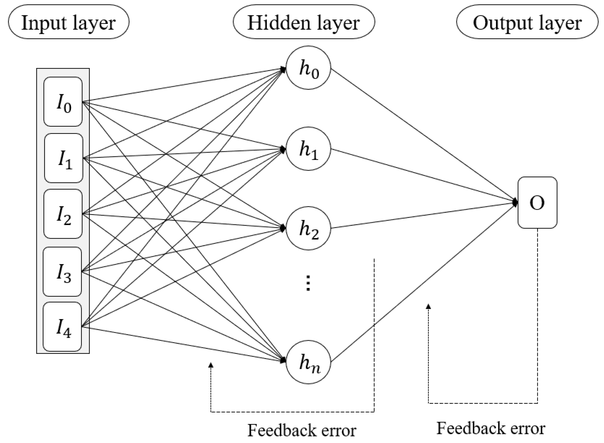
Mathematics 11 00314 g004
Figure 5. The layers of the RNN model.
Mathematics 11 00314 g005
Figure 6. The comparison of the MAPE of different models considering realized skewness and realized kurtosis.
Mathematics 11 00314 g006
Figure 7. The performance of ITM call options in different features (a) represents the LSTM with realized skewness, (b) represents the LSTM without realized skewness, (c) represents the LSTM with realized skewness and realized kurtosis.
Mathematics 11 00314 g007
Figure 8. The performance of ATM call options in different features (a) represents the LSTM with realized skewness, (b) represents the LSTM without realized skewness, (c) represents the LSTM with realized skewness and realized kurtosis.
Mathematics 11 00314 g008
Figure 9. The performance of OTM call options in different features (a) represents the LSTM with realized skewness, (b) represents the LSTM without realized skewness, (c) represents the LSTM with realized skewness and realized kurtosis.
Mathematics 11 00314 g009
Figure 10. The performance of ITM put options in different features (a) represents the LSTM with realized skewness, (b) represents the LSTM without realized skewness, (c) represents the LSTM with realized skewness and realized kurtosis.
Mathematics 11 00314 g010
Figure 11. The performance of ATM put options in different features (a) represents the LSTM with realized skewness, (b) represents the LSTM without realized skewness, (c) represents the LSTM with realized skewness and realized kurtosis.
Mathematics 11 00314 g011
Figure 12. The performance of OTM put options in different features (a) represents the LSTM with realized skewness, (b) represents the LSTM without realized skewness, (c) represents the LSTM with realized skewness and realized kurtosis.
Mathematics 11 00314 g012
Figure 13. The pricing performance of ITM call options on each model, (a) stands for the LSTM model, (b) stands for the BS model, (c) stands for the SVM model, (d) stands for the Ran-dom forests model, (e) stands for the RNN model.
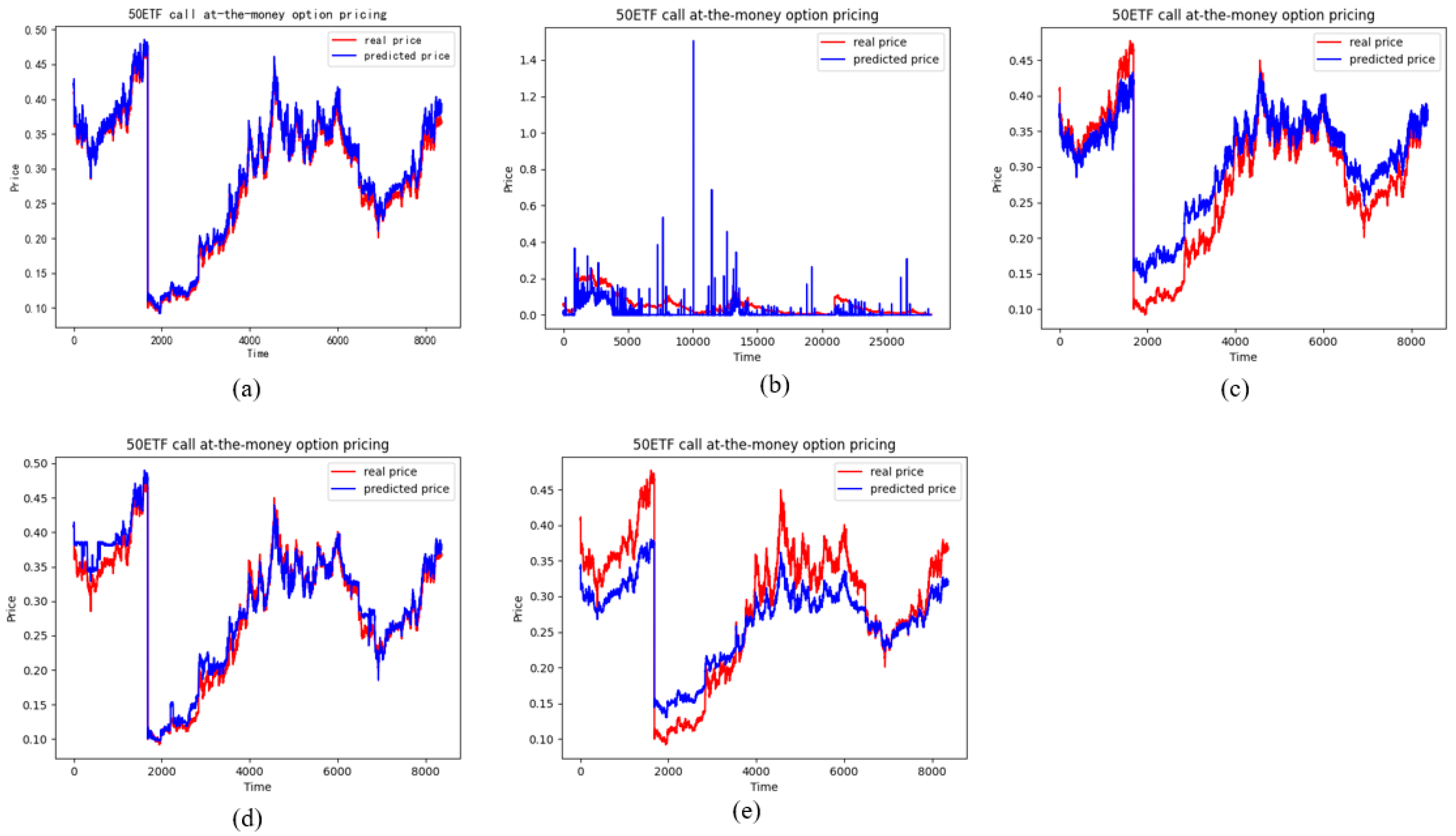
Mathematics 11 00314 g013
Figure 14. The pricing performance of ATM call options on each model (a) stands for the LSTM model, (b) stands for the BS model, (c) stands for the SVM model, (d) stands for the Random forests model, (e) stands for the RNN model.
Mathematics 11 00314 g014
Figure 15. The pricing performance of OTM call options on each model (a) stands for the LSTM model, (b) stands for the BS model, (c) stands for the SVM model, (d) stands for the Random forests model, (e) stands for the RNN model.
Mathematics 11 00314 g015
Figure 16. The pricing performance of ITM put options on each model (a) stands for the LSTM model, (b) stands for the BS model, (c) stands for the SVM model, (d) stands for the Random forests model, (e) stands for the RNN model.
Mathematics 11 00314 g016
Figure 17. The pricing performance of ATM put options on each model (a) stands for the LSTM model, (b) stands for the BS model, (c) stands for the SVM model, (d) stands for the Random forests model, (e) stands for the RNN model.
Mathematics 11 00314 g017
Figure 18. The pricing performance of OTM put options on each model (a) stands for the LSTM model, (b) stands for the BS model, (c) stands for the SVM model, (d) stands for the Random forests model, (e) stands for the RNN model.
Mathematics 11 00314 g018
Table 1. Hyperparameter of each model.
LSTMRNN
Activation functionRELURELU
Loss functionMSEMSE
Neurons[200, 200, 200, 200, 200, 1][200, 200, 200, 200, 200, 1]
Learning rate0.0010.001
OptimizerAdamAdam
Table 2. Description of moneyness.
StateMoneyness
Call optionITM>1.03
ATM0.97~1.03
OTM<0.97
Put optionITM<0.97
ATM0.97~1.03
OTM>1.03
Table 3. Statistics of ETF50 Call options sorted by moneyness.
Moneyness rSKMaturityRealized VolatilityRealized SkewnessRealized
Kurtosis
ITMcount70205702057020570205702057020570205
mean0.01393.61193.231756.47800.04110.00492.2384
std0.00590.14770.14990.14010.09481.13940.7893
min0.00613.3042.90880.0006−2.23611
max0.03284.0963.42373.97602.23615
ATMcount83637836378363783637836378363783637
mean0.014423.61813.493258.08460.03450.01992.2216
std0.00630.15290.09490.13740.07711.11120.777
min0.00613.3043.25380.0006−2.23611
max0.03284.0963.62373.97602.23615
OTMcount222532222532222532222532222532222532222532
mean0.01633.62423.742769.16480.03380.01512.2193
std0.00630.15690.1220.15940.07781.10950.7772
min0.00613.3043.4580.0006−2.23611
max0.03284.0963.92373.9762.23615
Table 4. Statistics of ETF50 Put options sorted by moneyness.
Moneyness rSKMaturityRealized VolatilityRealized SkewnessRealized
Kurtosis
ITMcount153988153988153988153988153988153988153988
mean0.01743.68413.712858.66330.03970.00712.2123
std0.00620.15290.13440.13890.09391.10930.7664
min0.00613.3043.4580.0006−2.23611
max0.03284.0963.92373.9762.23615
ATMcount103716103716103716103716103716103716103716
mean0.01543.63173.459664.85110.03460.01922.2207
std0.00640.15760.11340.14630.08131.10990.7756
min0.00613.3043.25380.0006−2.23611
max0.03284.0963.62363.9762.23615
OTMcount145085145085145085145085145085145085145085
mean0.0153.59793.177477.72590.03540.01642.2283
std0.00620.15020.15750.16710.08831.11940.7853
min0.00613.3042.90880.0007−2.23611
max0.03284.0963.42373.9762.23615
Table 5. Pricing error of LSTM without realized skewness.
MetricsCall OptionsPut Options
ITMATMOTMITMATMOTM
MSE0.00670.02890.02610.04420.00470.0019
RMSE0.81971.70031.61492.10270.68760.4307
MAE0.64371.52251.39051.87320.40640.2506
MAPE1.16115.286628.059225.167520.121746.2594
Note: All values are multiplied by a factor of 100.
Table 6. Pricing error of LSTM with realized skewness.
MetricsCall OptionsPut Options
ITMATMOTMITMATMOTM
MSE0.01180.0060.0150.02070.00360.0017
−76.12%79.24%42.53%53.17%23.40%10.53%
RMSE1.08750.77611.22571.4380.60350.4113
−32.67%54.36%24.10%31.61%12.23%4.50%
MAE0.90530.62531.04541.31980.35420.2331
−40.64%58.96%24.82%29.54%12.84%6.98%
MAPE1.7912.386819.889816.063416.757928.8013
−54.25%54.85%29.11%36.17%16.72%37.74%
Note: All values are multiplied by a factor of 100. The second line of each item is the percentage reduction per metric compared with LSTM without realized skewness. A negative value means the metric is higher than the previous value.
Table 7. Pricing error of LSTM with realized skewness and realized kurtosis.
MetricsCall OptionsPut Options
ITMATMOTMITMATMOTM
MSE0.01380.00540.02820.03050.00450.0015
−16.64%9.31%−87.94%−47.46%−24.81%10.70%
RMSE1.17320.73771.67901.74710.67030.3896
−7.88%4.95%−36.99%−21.50%−11.07%5.27%
MAE0.92420.59171.45371.53900.37510.2196
−2.09%5.37%−39.06%−16.61%−5.90%5.81%
MAPE1.60192.315129.047916.642016.775229.6484
10.56%3.01%−46.04%−3.60%−0.10%−2.94%
Note: All values are multiplied by a factor of 100. The second line of each item is the percentage reduction per metric compared with the LSTM containing realized skewness. A negative value means the metric is higher than the previous value.
Table 8. Pricing error of ITM options estimated using different models when using realized skewness.
ModelsITM Call Options ITM Put Options
MSERMSEMAEMAPE MSERMSEMAEMAPE
BS33.688558.041855.997399.9041 0.40376.35405.796064.2859
SVM0.12213.49462.86615.5627 0.35625.96815.767376.0187
RF0.02091.44740.98291.8028 0.01131.06310.855511.7190
RNN0.55447.44606.296510.6978 0.20934.57474.343356.2957
LSTM0.01181.08750.90531.7910 0.02071.43801.319816.0634
Note: ‘RF’ stands for Random forests model and all values are multiplied by a factor of 100.
Table 9. Pricing error of ATM options estimated using different models when using realized skewness.
ModelsATM Call Options ATM Put Options
MSERMSEMAEMAPE MSERMSEMAEMAPE
BS0.33035.74714.112297.2872 0.10953.30952.2106104.2794
SVM0.12573.54573.089515.1358 0.57187.56177.4347921.8113
RF0.02571.60231.20724.6944 0.00640.79890.515130.4049
RNN0.17644.19983.628613.8309 0.04582.14052.0417173.6328
LSTM0.00600.77610.62532.3868 0.00360.60350.354216.7579
Note: ‘RF’ stands for Random forests model and all values are multiplied by a factor of 100.
Table 10. Pricing error of OTM options estimated using different models when using realized skewness.
ModelsOTM Call Options OTM Put Options
MSERMSEMAEMAPE MSERMSEMAEMAPE
BS2.238514.961512.1928271.6490 0.01541.24130.7371107.8957
SVM0.27725.26504.896675.7476 0.83539.13959.11243293.3315
RF0.06272.50381.824722.9774 0.00230.48320.284534.4681
RNN0.16614.07533.805672.5007 0.00480.69390.6531183.8504
LSTM0.01501.22571.045419.8898 0.00170.41130.233128.8013
Note: ‘RF’ stands for Random forests model and all values are multiplied by a factor of 100.
Table 11. Pricing error of ITM options estimated using different models when using realized skewness and realized kurtosis.
ModelsITM Call Options ITM Put Options
MSERMSEMAEMAPE MSERMSEMAEMAPE
BS33.688558.041855.997399.9041 0.40376.35405.796064.2859
SVM0.12263.50162.86885.6109 0.35135.92675.718675.6203
RF0.02081.44060.98121.7970 0.01121.05760.849711.6567
RNN0.59877.73736.517511.1190 0.30305.50435.303069.5781
LSTM0.01381.17320.92421.6019 0.03051.74711.539016.6420
Note: ‘RF’ stands for Random forests model and all values are multiplied by a factor of 100.
Table 12. Pricing error of ATM options estimated using different models when using realized skewness and realized kurtosis.
ModelsATM Call Options ATM Put Options
MSERMSEMAEMAPE MSERMSEMAEMAPE
BS0.33035.74714.112297.2872 0.10953.30952.2106104.2794
SVM0.11393.37442.902214.3229 0.55967.48067.3462912.8136
RF0.02531.59151.20084.6725 0.00580.75840.492529.7101
RNN0.18154.26053.680214.1544 0.04722.17312.1188200.7604
LSTM0.00540.73770.59172.3151 0.00450.67030.375116.7752
Note: ‘RF’ stands for Random forests model and all values are multiplied by a factor of 100.
Table 13. Pricing error of OTM options estimated using different models when using realized skewness and realized kurtosis.
ModelsOTM Call Options OTM Put Options
MSERMSEMAEMAPE MSERMSEMAEMAPE
BS2.238514.961512.1928271.6490 0.01541.24130.7371107.8957
SVM0.28565.34464.977877.0127 0.83539.13959.11243293.3115
RF0.06282.50531.824123.0268 0.00240.48490.285334.4997
RNN0.21634.65034.396283.6558 0.00910.95440.8765238.5260
LSTM0.02821.67901.453729.0479 0.00150.38960.219629.6484
Note: ‘RF’ stands for Random forests model and all values are multiplied by a factor of 100.
Disclaimer/Publisher’s Note: The statements, opinions and data contained in all publications are solely those of the individual author(s) and contributor(s) and not of MDPI and/or the editor(s). MDPI and/or the editor(s) disclaim responsibility for any injury to people or property resulting from any ideas, methods, instructions or products referred to in the content.

