Singularity, Observability and Statistical Independence in the Context of Chaotic Systems

Abstract

Pseudorandom number generators (PRNGs) have always been a central research topic in data science, and chaotic dynamical systems are one of the means to obtain scientifically proven data. Chaotic dynamical systems have the property that they have a seemingly unpredictable and random behavior obtained by making use of deterministic laws. The current paper will show how several notions used in the study of chaotic systems—statistical independence, singularity, and observability—can be used together as a suite of test methods for chaotic systems with high potential of being used in the PRNG or cryptography fields. In order to address these topics, we relied on the adaptation of the observability coefficient used in previous papers of the authors, we calculated the singularity areas for the chaotic systems considered, and we evaluated the selected chaotic maps from a statistical independence point of view. By making use of the three notions above, we managed to find strong correlations between the methods proposed, thus supporting the idea that the resulting test procedure is consistent. Future research directions consist of applying the proposed test procedure to other chaotic systems in order to gather more data and formalize the approach in a test suite that can be used by the data scientist when selecting the best chaotic system for a specific use (PRNG, cryptography, etc.).

1. Introduction

People have needed to communicate sensitive subjects among themselves from the beginning of time [1], and it was of paramount importance that no one else apart from the intended recipient of the message could understand the meaning [2]. Cryptography was born as a means to allow the involved parties to maintain the confidentiality of the shared information, even when there is a man-in-the-middle who wants to capture and decipher the message [3,4]. Confidentiality remains one of the main pillars and interest topics in cryptography [5,6], and the ramifications of this essential domain in the past decades are very vast and far-reaching.

One of the enablers of a good cryptographic system is represented by the use of dynamical chaotic systems [7,8,9]. Nonlinear dynamical chaotic systems are a hot area of investigation, independent on their form: with or without a stable equilibrium point [10]. FPGA implementations of different chaotic systems are also of interest, as they are the first step when transforming theory into practical applications in real life [11]. Different fields, such as robotics, encryption, and wired or wireless communication, can benefit from the results obtained in this new active research topic area represented by the study of chaotic dynamical systems [3].

Nevertheless, not all chaotic systems share the same cryptographic properties [12,13], and there is not such a concept of “one size fits all applications”. The aim of this paper is to shed some light on this by analyzing the Clifford, Tinkerbell, and Ikeda maps from three different perspectives: observability [14,15,16], singularity [17], and statistical independence [18,19]. Moreover, the aim is to find a connection/correlation among the three approaches such that when a chaotic system passes the three “tests”, then one can say with a higher degree of certainty that the respective system stands a chance as a good cryptographic system.

The original contribution of this paper is that it analyzes in detail and as a whole the three concepts noted above, which are usually treated separately/independently, and manages to link them together to create a unified and stronger perspective of a dynamical chaotic map to be used in cryptography. Investigating the observability, singularity, and statistical independence alone (one by one) can be a disadvantage, being similar to locally optimizing a function; this is the main benefit of this paper, that it achieves a unified analysis of a dynamical system by combining three different strong perspectives.

Section 2 presents the existing state-of-the-art results that were the starting point of this research. Section 3 goes further and adds a new layer of knowledge on the observability, singularity, and statistical independence topics. The main results and other potential research directions are presented in Section 4.

2. Theoretical Background

A simple definition of a dynamical system can be that it is a rule for time evolution on a state space. An example of such a system is the Lorenz system. The Lorenz system is defined by a set of three differential equations shown below (continuous representation—(1) and discrete representation—(2); $\mathsf{\Delta }t=1/F_s$). The merits for this system of differential equations can be attributed to Edward Lorenz, a U.S. meteorologist, who wanted to find a way to express the changes in wind speed and temperature. The way he managed to accomplish this goal was through the set of three differential equations described below. Subsequent computer validations proved that the equations found by Lorenz were leading to a complex system where small changes in the set of initial conditions led to completely different results in time. The solutions stemming from this chaotic system can always be found evolving around a structure named a strange attractor fractal [17]. A set of parameters used to ensure a chaotic behavior occurs are $a=10$, $b=8/3$, and $c=28$ [20]; x, y, and z are the state variables for the Lorenz system.

$$\left\{\begin{array}{c}\frac{dx}{dt}=a·(y-x)\hfill \\ \frac{dy}{dt}=x·(c-z)-y\hfill \\ \frac{dz}{dt}=x·y-b·z\hfill \end{array}\right.$$

(1)

$$\left\{\begin{array}{c}\frac{x_{k+1}-x_k}{\mathsf{\Delta }t}=a·(y_k-x_k)\hfill \\ \frac{y_{k+1}-y_k}{\mathsf{\Delta }t}=x_k·(c-z_k)-y_k\hfill \\ \frac{z_{k+1}-z_k}{\mathsf{\Delta }t}=x_k·y_k-b·z_k\hfill \end{array}\right.$$

(2)

The main theoretical concepts used in this paper are described next. Observability is the capacity to determine the system’s states or the time evolution of the input/output in any finite, non-zero time interval, based on the the system’s history. In other words, observability allows the observation and analysis of the internal states of the system just by having access to its input/output space. Observability in the context of an n-dimensional chaotic system means that, having involved a series of values generated by the state variables of the system, one can reconstruct the phase space of the system [21]. Note that the concept of observability is discussed in the hypothesis that the system parameters are known. The idea of observability for multi-dimensional systems is discussed at length in [22,23].

The definition of the singularity manifold for dynamical systems, $S_{\overline{O}}$, can be seen from different perspectives, and it is closely related to the notion of observability. The space area where the observability property of the system is lost for a specific state variable represents the singularity manifold for that variable. The system is not observable in that area. The fact that a system is fully observable is of paramount importance in cryptography and that is why determining the singularity manifolds will be one of the angles we will investigate in this paper [24].

Next is presented the approach used to determine when statistical independence is reached. Vlad et al. [18] defined a test procedure that can conclude whether two random variables are statistically independent by making use of a Pearson-like test procedure and a visual assessment as well. An improved statistical independence test was proposed by the same group of authors [19] who made use in an innovative way of the chi square test [25] in order to check the compliance of two experimental datasets with the Gaussian bivariate probability law.

The datasets that will be analyzed in this paper from the point of view of statistical independence will be called X and Y and will be collected from the solution space of the investigated dynamical systems. According to the test procedure described in [18], X and Y will be converted into two new datasets (U and V) that are distributed according to a Gaussian probability law. The spatial chi square test proposed in [19] will take statistical independence decisions based on the new datasets (U and V). Simply put, the test will verify whether U and V satisfy the standard normal bivariate probability law (3). If the answer is Yes, then the original X and Y are statistically independent as well.

$$p(u,v)={\displaystyle \frac{1}{2\pi }}{e}^{-{\displaystyle \frac{u^2+v^2}{2}}}$$

(3)

The two statistical hypotheses of the spatial chi square test are noted below:

• $H_0$—the null hypothesis: the two datasets (U and V) follow the bivariate normal probability law specified in (3), i.e., U and V (and implicitly X and Y) are statistically independent.
• $H_1$—the alternative hypothesis: the two datasets (U and V) do not follow the bivariate normal probability law specified in (3), i.e., U and V (and implicitly X and Y) are not statistically independent

The first step when applying the chi square test is to group the experimental data in classes, and the number of occurrences in each class is counted. Next, the test value is calculated based on (4):

$$z=\sum _{k=1}^M{\displaystyle \frac{{(m_k-N{P}_k)}^2}{N{P}_k}}$$

(4)

where the number of classes used is denoted by M, $m_k$ represents the number of occurrences in class k, i.e., the count of the experimental data points from U and V that belong to the respective class. Furthermore, the volume of data is N (total number of experimental data points $(u_i,v_i)$), $P_k$ is the reference probability for class k, assuming that variables U and V are jointly Gaussian. The chosen chi square test used in this paper was a bilateral test with a statistical significance level $\alpha =0.05$.

The number of classes of the spatial chi square test, M, is dependent on the volume of experimental data, N, as can be observed in

Table 1. Data dependency between the number of classes (M) and data volume (N).

Data Volume (N)	Number of Classes (M)	Number of Circles	Number of Sectors
10,000	48	6	8
40,000	288	16	18
100,000	672	24	28
1,000,000	3440	40	86

. The first column notes the data volume, N; the second column includes the number of classes, M, for a specific N value. The next two columns reference the number of sectors and circles used to reach the number of classes from column 2. In fact, the value in column 2 is equal to the product of the values stored in columns 3 and 4. One can choose to use as many M classes for the algorithm as desired. The only condition is to have a minimum amount of occurrences in each class, this being a prerequisite for the chi square test [19].

3. Experimental Results

3.1. Dynamical Systems

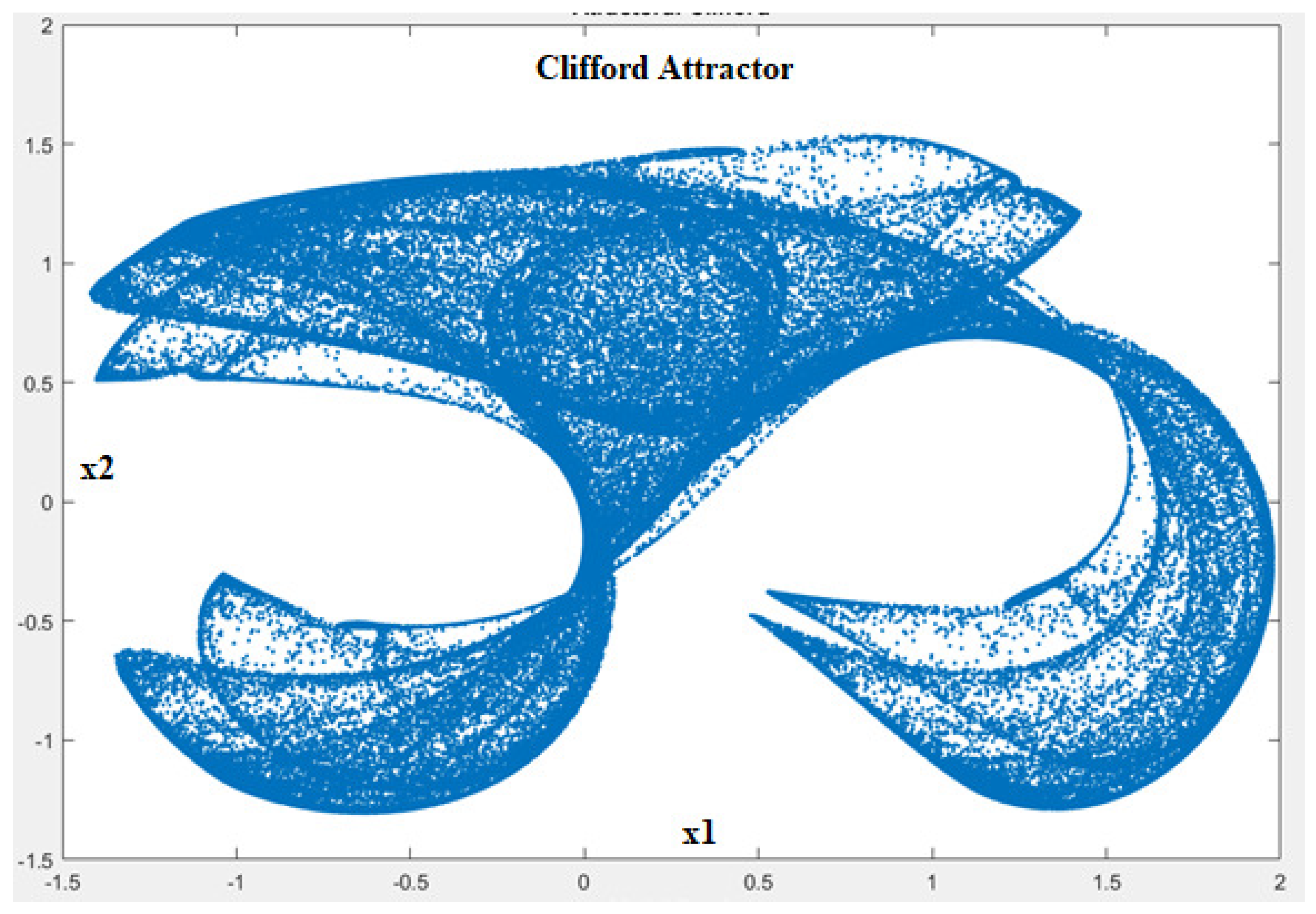
The Clifford dynamical system is defined by Equation (5).

$$\left\{\begin{array}{c}{x}_1^{+}=sin(a·x_2)+c·cos(a·x_1)\hfill \\ x_2^{+}=sin(b·x_1)+d·cos(b·x_2)\hfill \end{array}\right.$$

(5)

If $x_1$ and $x_2$ are the values of the system at moment t in time, $x_1^{+}$ and $x_2^{+}$ are the values of the system at the next moment in time, $t+1$. For a selection of system parameters that are known to lead to a chaotic behavior ($a=-1.4$, $b=1.6$, $c=1$, $d=0$) and $x_1\left(0\right)=0.1$ and $x_2\left(0\right)=0.1$ as the set of initial conditions, the first 100,000 iterations calculated based on (5) are depicted in Figure 1.

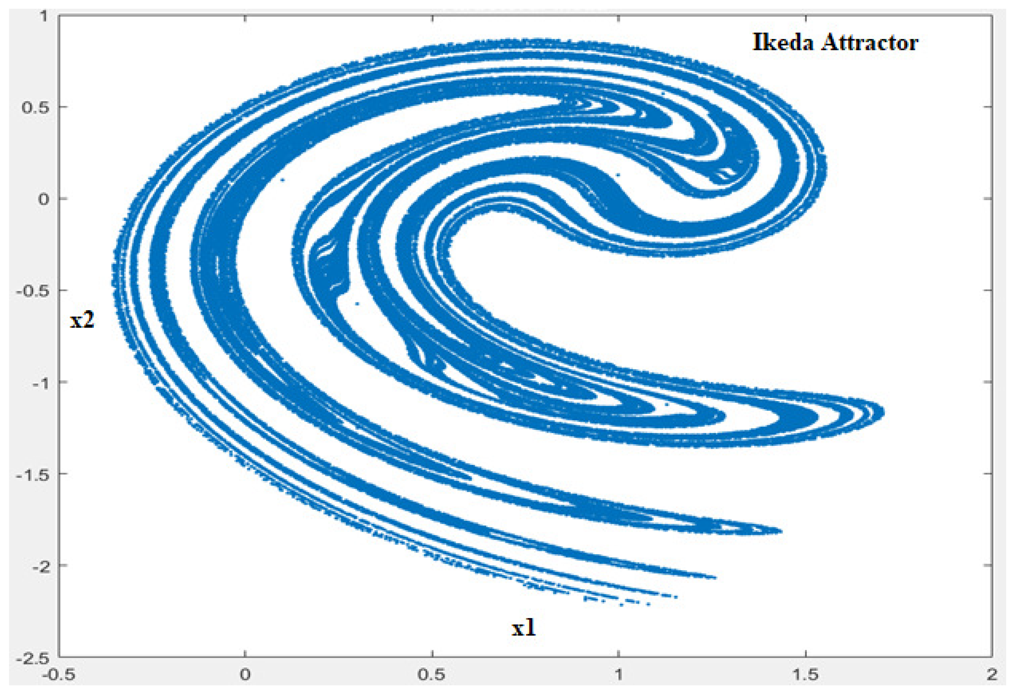
The Ikeda dynamical system is defined by Equation (6).

$$\left\{\begin{array}{c}{x}_1^{+}=1+u·[x_1·cos\left(t\right)-x_2·sin\left(t\right)]\hfill \\ x_2^{+}=u·[x_1·sin\left(t\right)+x_2·cos\left(t\right)]\hfill \\ t=0.4-{\displaystyle \frac{6}{1+x_1^2+x_2^2}}\hfill \end{array}\right.$$

(6)

A parameter that is known to lead to a chaotic behavior is $u=0.9$ and for the set of initial conditions $x_1\left(0\right)=0.1$ and $x_2\left(0\right)=0.12$, the first 100,000 iterations calculated based on (6) are depicted in Figure 2.

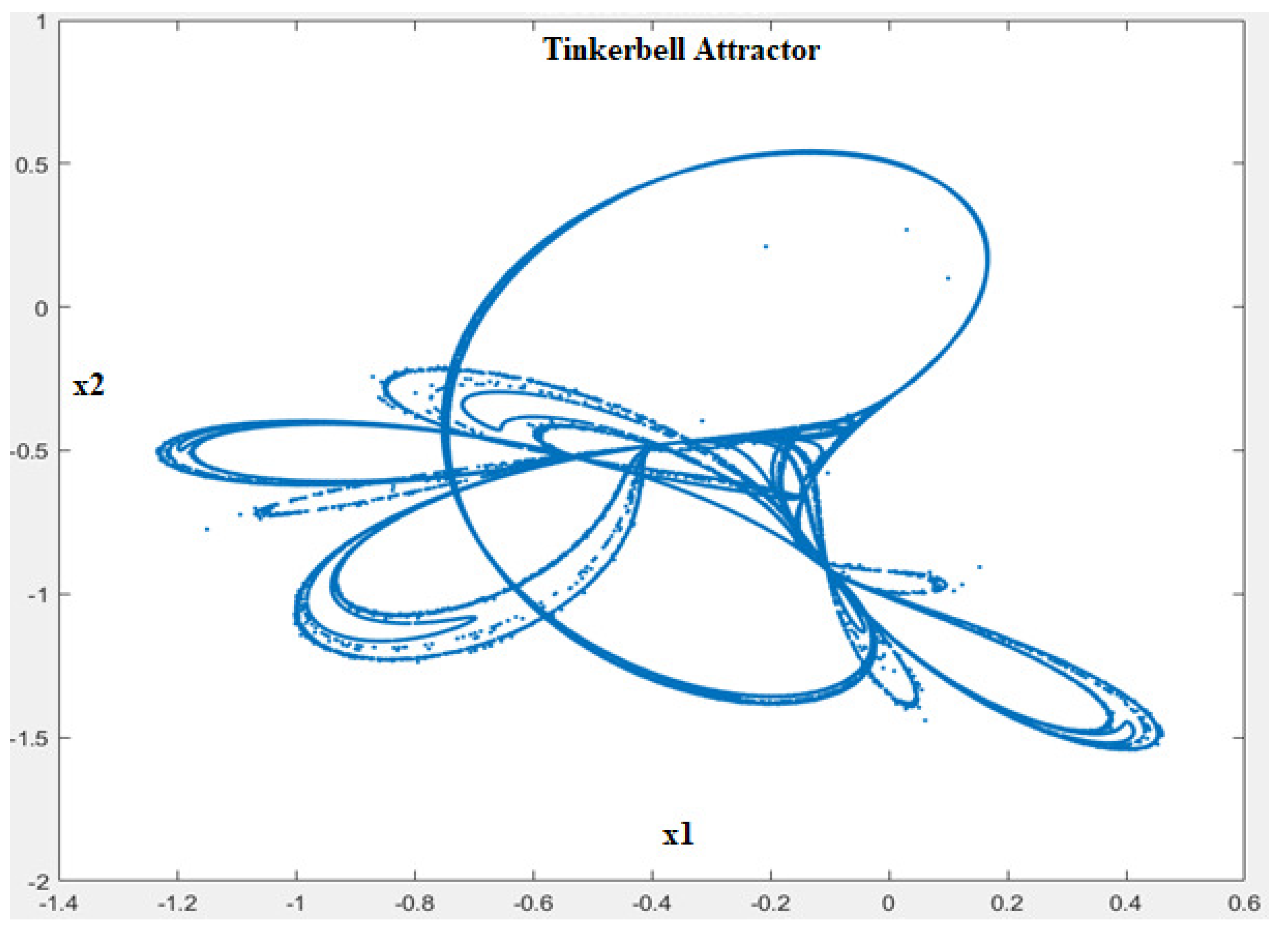
The Tinkerbell dynamical system is defined by Equation (7).

$$\left\{\begin{array}{c}{x}_1^{+}=x_1^2-x_2^2+a·x_1+b·x_2\hfill \\ x_2^{+}=2·x_1·x_2+c·x_1+d·x_2\hfill \end{array}\right.$$

(7)

For a selection of system parameters that are known to lead to a chaotic behavior ($a=0.9$, $b=-0.6013$, $c=2$, $d=0.5$) and $x_1\left(0\right)=0.1$ and $x_2\left(0\right)=0.1$ as the set of initial conditions, the first 100,000 iterations calculated based on (7) are depicted in Figure 3.

3.2. Observability

The procedure used to calculate the observability coefficient for each of the dynamical systems selected is shown next. The first system analyzed is the Clifford map described in (5). The steps followed are presented next and are based on the results from [14,24]:

• Create the fluency matrix $F_{ij}$, where each value depends on the terms from the equations describing the chaotic map:

  (a)

  1 for linear dependency;

  (b)

  $\overline{1}$ for non-linear dependency;

  (c)

  $\lambda ={\displaystyle \frac{1}{2·\pi }}$ for trigonometric dependency.

• $F_{ij}=\left[\begin{array}{cc}\lambda & \lambda \\ \lambda & \lambda \end{array}\right]$
• Select a state variable to rebuild the dynamics of the system; define the column array $C_{1,i}$, with 1 on the ith position and 0 elsewhere: $c_{1,1}=\left[\begin{array}{c}1\\ 0\end{array}\right]$ and $c_{1,2}=\left[\begin{array}{c}0\\ 1\end{array}\right]$
• Create matrix $H_{1,i}$ by multiplying each line from $F_{ij}$ with the corresponding element from array $c_{1,i}$ and replacing element $x_{ii}$ with a · $H_{1,1}=\left[\begin{array}{cc}·& \lambda \\ 0& 0\end{array}\right]$ for $x_1$ and $H_{1,2}=\left[\begin{array}{cc}0& 0\\ \lambda & ·\end{array}\right]$ for $x_2$
• Further on, variable $p_{1,i}$ will count the number of linear elements from $H_{1,i}$ and $q_{1,i}$ the number of non-linear and trigonometric elements from $H_{1,i}$, for each state variable $x_1$ or $x_2$.

  $$\left\{\begin{array}{c}{p}_{1,1}=0\hfill \\ q_{1,1}=1\hfill \end{array}\right.\mathrm{for}{x}_1\mathrm{and}\left\{\begin{array}{c}{p}_{1,2}=0\hfill \\ q_{1,2}=1\hfill \end{array}\right.\mathrm{for}{x}_2.$$
• Next, the · from matrix $H_{1,i}$ is replaced with the corresponding element from the fluency matrix, and the resulting matrix is transposed:
  $H_{11}=\left[\begin{array}{cc}\lambda & \lambda \\ 0& 0\end{array}\right]$→$H_{11}^T=\left[\begin{array}{cc}\lambda & 0\\ \lambda & 0\end{array}\right]$ for $x_1$
  $H_{12}=\left[\begin{array}{cc}0& 0\\ \lambda & \lambda \end{array}\right]$→$H_{12}^T=\left[\begin{array}{cc}0& \lambda \\ 0& \lambda \end{array}\right]$ for $x_2$
• The column arrays $c_{2,i}$ are created by summing the elements on the lines of the previously defined matrices $H_{1,i}^T$ (1 and $\overline{1}$ are considered as 1):
  $c_{2,1}=\left[\begin{array}{c}\lambda \\ \lambda \end{array}\right]$ and $c_{2,2}=\left[\begin{array}{c}\lambda \\ \lambda \end{array}\right]$
• Matrices $H_{2,i}$ are created by replacing any non-zero element from $H_{1,i}^T$ with a · and the zero elements with the corresponding terms from the fluency matrix multiplied by the corresponding element from array $c_{2,i}$
  $H_{21}=\left[\begin{array}{cc}·& \lambda \\ ·& \lambda \end{array}\right]$ for $x_1$ and $H_{22}=\left[\begin{array}{cc}\lambda & ·\\ \lambda & ·\end{array}\right]$ for $x_2$
• The expression $p_{2,i}$ will count the number of linear elements from $H_{2,i}$ and $q_{2,i}$ the number of non-linear and trigonometric elements from $H_{2,i}$, for each state variable $x_i$.

  $$\left\{\begin{array}{c}{p}_{2,1}=0\hfill \\ q_{2,1}=2\hfill \end{array}\right.\mathrm{for}{x}_1\mathrm{and}\left\{\begin{array}{c}{p}_{2,2}=0\hfill \\ q_{2,2}=2\hfill \end{array}\right.\mathrm{for}{x}_2.$$
• The observability coefficient ${\eta }_i$ (for each state variable) is calculated with the following formula:

  $${\eta }_i={\displaystyle \frac{1}{2}}·\left[{\displaystyle \frac{p_{i,1}}{p_{i,1}+q_{i,1}}}+{\displaystyle \frac{q_{i,1}}{{(p_{i,1}+q_{i,1})}^3}}+{\displaystyle \frac{p_{i,2}}{p_{i,2}+q_{i,2}}}+{\displaystyle \frac{q_{i,2}}{{(p_{i,2}+q_{i,2})}^2}}\right]$$

  (8)
• By taking into account the p and q values previously calculated, and the fact that

  $$\left\{\begin{array}{c}{p}_k+q_k=1+q_k\mathrm{for}{p}_k=0\mathrm{and}\mathrm{dependance}\mathrm{non}-\mathrm{trigonometric}\hfill \\ p_k+q_k=\lambda +q_k={\displaystyle \frac{1}{2·\pi }}\mathrm{for}{p}_k=0\mathrm{and}\mathrm{dependance}\mathrm{trigonometric}\hfill \end{array}\right.$$

  one can easily find that

  $$\left\{\begin{array}{c}{\eta }_1=0.54\hfill \\ {\eta }_2=0.54\hfill \end{array}\right.$$

The system analyzed next from an observability perspective is the Ikeda map. The steps followed are similar to the ones for the Clifford map and the results are presented below:

• By taking into account that the equations from (6) are not purely trigonometric as it was the case for Clifford, they were considered as non-linear, and the fluency matrix $F_{ij}=\left[\begin{array}{cc}\overline{1}& \overline{1}\\ \overline{1}& \overline{1}\end{array}\right]$
• Choose a state variable to reconstruct the dynamics of the system; define the column array $C_{1,i}$, with 1 on the ith position and 0 elsewhere: $c_{1,1}=\left[\begin{array}{c}1\\ 0\end{array}\right]$ and $c_{1,2}=\left[\begin{array}{c}0\\ 1\end{array}\right]$
• Create matrix $H_{1,i}$ by multiplying each line from $F_{ij}$ with the corresponding element from array $c_{1,i}$ and replacing element $x_{ii}$ with a · $H_{1,1}=\left[\begin{array}{cc}·& \overline{1}\\ 0& 0\end{array}\right]$ for $x_1$ and $H_{1,2}=\left[\begin{array}{cc}0& 0\\ \overline{1}& ·\end{array}\right]$ for $x_2$
• Variable $p_{1,i}$ will count the number of linear elements from $H_{1,i}$ and $q_{1,i}$ the number of non-linear and trigonometric elements from $H_{1,i}$, for each state variable $x_1$ or $x_2$.

  $$\left\{\begin{array}{c}{p}_{1,1}=0\hfill \\ q_{1,1}=1\hfill \end{array}\right.\mathrm{for}{x}_1\mathrm{and}\left\{\begin{array}{c}{p}_{1,2}=0\hfill \\ q_{1,2}=1\hfill \end{array}\right.\mathrm{for}{x}_2.$$
• The · from matrix $H_{1,i}$ is replaced with the corresponding element from the fluency matrix, and the resulting matrix is transposed:
  $H_{11}=\left[\begin{array}{cc}\overline{1}& \overline{1}\\ 0& 0\end{array}\right]$→$H_{11}^T=\left[\begin{array}{cc}\overline{1}& 0\\ \overline{1}& 0\end{array}\right]$ for $x_1$
  $H_{12}=\left[\begin{array}{cc}0& 0\\ \overline{1}& \overline{1}\end{array}\right]$→$H_{12}^T=\left[\begin{array}{cc}0& \overline{1}\\ 0& \overline{1}\end{array}\right]$ for $x_2$
• The column arrays $c_{2,i}$ are created by summing the elements on the lines of the previously defined matrices $H_{1,i}^T$ (1 and $\overline{1}$ are considered as 1):
  $c_{2,1}=\left[\begin{array}{c}1\\ 1\end{array}\right]$ and $c_{2,2}=\left[\begin{array}{c}1\\ 1\end{array}\right]$
• Matrices $H_{2,i}$ are created by replacing any non-zero element from $H_{1,i}^T$ with a · and the zero elements with the corresponding terms from the fluency matrix multiplied by the corresponding element from array $c_{2,i}$
  $H_{21}=\left[\begin{array}{cc}·& \overline{1}\\ ·& \overline{1}\end{array}\right]$ for $x_1$ and $H_{22}=\left[\begin{array}{cc}\overline{1}& ·\\ \overline{1}& ·\end{array}\right]$ for $x_2$
• Variable $p_{2,i}$ will count the number of linear elements from $H_{2,i}$ and $q_{2,i}$ the number of non-linear and trigonometric elements from $H_{2,i}$, for each state variable $x_i$.

  $$\left\{\begin{array}{c}{p}_{2,1}=0\hfill \\ q_{2,1}=2\hfill \end{array}\right.\mathrm{for}{x}_1\mathrm{and}\left\{\begin{array}{c}{p}_{2,2}=0\hfill \\ q_{2,2}=2\hfill \end{array}\right.\mathrm{for}{x}_2.$$
• The observability coefficient ${\eta }_i$ (for each state variable) is calculated with the formula

  $${\eta }_i={\displaystyle \frac{1}{2}}·\left[{\displaystyle \frac{p_{i,1}}{p_{i,1}+q_{i,1}}}+{\displaystyle \frac{q_{i,1}}{{(p_{i,1}+q_{i,1})}^3}}+{\displaystyle \frac{p_{i,2}}{p_{i,2}+q_{i,2}}}+{\displaystyle \frac{q_{i,2}}{{(p_{i,2}+q_{i,2})}^2}}\right]$$

  (9)
• By taking into account the p and q values previously calculated, and the fact that

  $$\left\{\begin{array}{c}{p}_k+q_k=1+q_k\mathrm{for}{p}_k=0\mathrm{and}\mathrm{dependance}\mathrm{non}-\mathrm{trigonometric}\hfill \\ p_k+q_k=\lambda +q_k={\displaystyle \frac{1}{2·\pi }}\mathrm{for}{p}_k=0\mathrm{and}\mathrm{dependance}\mathrm{trigonometric}\hfill \end{array}\right.$$

  one can easily find that

  $$\left\{\begin{array}{c}{\eta }_1=0.17\hfill \\ {\eta }_2=0.17\hfill \end{array}\right.$$

The last system analyzed from an observability perspective is the Tinkerbell map. The main results are presented below:

• The fluency matrix looks different this time, being the result of a combination of linear and non-linear elements $F_{ij}=\left[\begin{array}{cc}\overline{1}& \overline{1}\\ 1& 1\end{array}\right]$
• Choose a state variable to reconstruct the dynamics of the system; define the column array $C_{1,i}$, with 1 on the ith position and 0 elsewhere: $c_{1,1}=\left[\begin{array}{c}1\\ 0\end{array}\right]$ and $c_{1,2}=\left[\begin{array}{c}0\\ 1\end{array}\right]$
• Create matrix $H_{1,i}$ by multiplying each line from $F_{ij}$ with the corresponding element from array $c_{1,i}$ and replacing element $x_{ii}$ with a · $H_{1,1}=\left[\begin{array}{cc}·& \overline{1}\\ 0& 0\end{array}\right]$ for $x_1$ and $H_{1,2}=\left[\begin{array}{cc}0& 0\\ 1& ·\end{array}\right]$ for $x_2$
• Variable $p_{1,i}$ will count the number of linear elements from $H_{1,i}$ and $q_{1,i}$ the number of non-linear and trigonometric elements from $H_{1,i}$, for each state variable $x_1$ or $x_2$.

  $$\left\{\begin{array}{c}{p}_{1,1}=0\hfill \\ q_{1,1}=1\hfill \end{array}\right.\mathrm{for}{x}_1\mathrm{and}\left\{\begin{array}{c}{p}_{1,2}=1\hfill \\ q_{1,2}=0\hfill \end{array}\right.\mathrm{for}{x}_2.$$
• The · from matrix $H_{1,i}$ is replaced with the corresponding element from the fluency matrix, and the resulting matrix is transposed:
  $H_{11}=\left[\begin{array}{cc}\overline{1}& \overline{1}\\ 0& 0\end{array}\right]$→$H_{11}^T=\left[\begin{array}{cc}\overline{1}& 0\\ \overline{1}& 0\end{array}\right]$ for $x_1$
  $H_{12}=\left[\begin{array}{cc}0& 0\\ 1& 1\end{array}\right]$→$H_{12}^T=\left[\begin{array}{cc}0& 1\\ 0& 1\end{array}\right]$ for $x_2$
• The column arrays $c_{2,i}$ are created by summing the elements on the lines of the previously defined matrices $H_{1,i}^T$ (1 and $\overline{1}$ are considered as 1):
  $c_{2,1}=\left[\begin{array}{c}1\\ 1\end{array}\right]$ and $c_{2,2}=\left[\begin{array}{c}1\\ 1\end{array}\right]$
• Matrices $H_{2,i}$ are created by replacing any non-zero element from $H_{1,i}^T$ with a · and the zero elements with the corresponding terms from the fluency matrix multiplied by the corresponding element from array $c_{2,i}$
  $H_{21}=\left[\begin{array}{cc}·& \overline{1}\\ ·& 1\end{array}\right]$ for $x_1$ and $H_{22}=\left[\begin{array}{cc}\overline{1}& ·\\ 1& ·\end{array}\right]$ for $x_2$
• The variable $p_{2,i}$ will count the number of linear elements from $H_{2,i}$ and $q_{2,i}$ the number of non-linear and trigonometric elements from $H_{2,i}$, for each state variable $x_i$.

  $$\left\{\begin{array}{c}{p}_{2,1}=1\hfill \\ q_{2,1}=1\hfill \end{array}\right.\mathrm{for}{x}_1\mathrm{and}\left\{\begin{array}{c}{p}_{2,2}=1\hfill \\ q_{2,2}=1\hfill \end{array}\right.\mathrm{for}{x}_2.$$
• The observability coefficient ${\eta }_i$ (for each state variable) is calculated with the formula

  $${\eta }_i={\displaystyle \frac{1}{2}}·\left[{\displaystyle \frac{p_{i,1}}{p_{i,1}+q_{i,1}}}+{\displaystyle \frac{q_{i,1}}{{(p_{i,1}+q_{i,1})}^3}}+{\displaystyle \frac{p_{i,2}}{p_{i,2}+q_{i,2}}}+{\displaystyle \frac{q_{i,2}}{{(p_{i,2}+q_{i,2})}^2}}\right]$$

  (10)
• By taking into account the p and q values previously calculated, and the fact that

  $$\left\{\begin{array}{c}{p}_k+q_k=1+q_k\mathrm{for}{p}_k=0\mathrm{and}\mathrm{dependance}\mathrm{non}-\mathrm{trigonometric}\hfill \\ p_k+q_k=\lambda +q_k={\displaystyle \frac{1}{2·\pi }}\mathrm{for}{p}_k=0\mathrm{and}\mathrm{dependance}\mathrm{trigonometric}\hfill \end{array}\right.$$

  one can easily find that

  $$\left\{\begin{array}{c}{\eta }_1=0.44\hfill \\ {\eta }_2=0.88\hfill \end{array}\right.$$

The results of the observability analysis are collated in

Table 2. Observability coefficients per state variable and chaotic system analyzed.

Chaotic System	${\mathit{\eta }}_1$ Observability Coefficient	${\mathit{\eta }}_2$ Observability Coefficient
Clifford	0.54	0.54
Ikeda	0.17	0.17
Tinkerbell	0.44	0.88

.

One can notice that the Tinkerbell observability coefficients are different for the two state variables, which is a different observation compared to the first two systems analyzed. A potential explanation can be the fact that the Tinkerbell system is described as a combination of linear and non-linear terms, compared to the Clifford and Ikeda maps, which were purely trigonometric or non-linear.

3.3. Singularity

Closely related to the concept of observability previously discussed is another important topic, discussed in the following paragraphs: singularity. A singularity manifold is the space where the observability property of the system vanishes. The desired outcome for cryptography is that the system is non-singular, meaning that it is completely observable from the perspective of the observed state variable, or $S_{\overline{O}}=\varnothing$.

The procedure used to determine the singularity areas for the three systems analyzed in this paper and the results obtained are presented next. The relationship between the space phase at the current iteration and the next one are depicted in (11) for the state variable $x_i$.

$${\mathsf{\Phi }}_i:\left\{\begin{array}{c}X=s=x_i\hfill \\ Y=s^{+}={x_i}^{+}\hfill \end{array}\right.$$

(11)

Variables X and Y correspond to iterations k and $k+1$; $O_i$ is the observability matrix corresponding to the state variable $x_i$ of a non-linear dynamical system and is equal to the Jacobian of the map ${\mathsf{\Phi }}_i$; $O_i$ is expressed in (12).

$$O_i=\left(\begin{array}{cc}{\displaystyle \frac{\delta X}{\delta x_1}}& {\displaystyle \frac{\delta X}{\delta x_2}}\\ {\displaystyle \frac{\delta Y}{\delta y_1}}& {\displaystyle \frac{\delta Y}{\delta y_2}}\end{array}\right)$$

(12)

The chaotic system is fully observable when $det(O_i$) is never 0. That means that the map ${\mathsf{\Phi }}_i$ is inversible and the system can be always written in an iterative form like in (13).

$$\left\{\begin{array}{c}{X}^{+}=Y\hfill \\ Y^{+}=F_i(X,Y)\hfill \end{array}\right.$$

(13)

where function $F_i$ has no singularities, and index i designates the state variable. If the aforementioned condition is not met, the system is not fully observable. The singularity manifold for the state variable $x_i$ is expressed in mathematical form in (14).

$$S_{{\overline{O}}_i}=\{(x_1,x_2)\in \mathbb{R}|det\left(O_i\right)=0\}$$

(14)

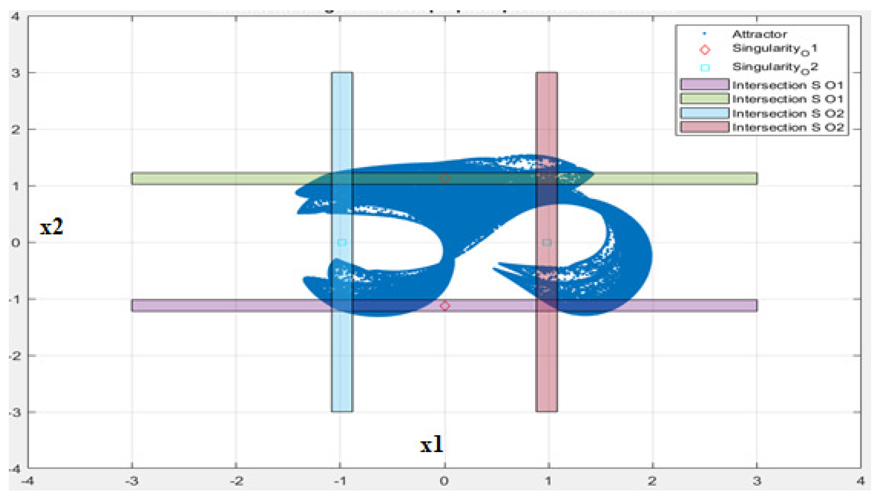
For the Clifford system, the singularity manifolds for both state variables are calculated in (15)–(18):

$${\mathsf{\Phi }}_1:\left\{\begin{array}{c}X=s=x_1\hfill \\ Y=s^{+}={x_1}^{+}=sin(a·x_2)+c·cos(a·x_1)\hfill \end{array}\right.$$

(15)

$$O_1=\left(\begin{array}{cc}1& 0\\ -c·a·sin(a·x_1)& a·cos(a·x_2)\end{array}\right)$$

(16)

$${\mathsf{\Phi }}_2:\left\{\begin{array}{c}X=s=x_2\hfill \\ Y=s^{+}={x_2}^{+}=sin(a·x_1)+d·cos(b·x_2)\hfill \end{array}\right.$$

(17)

$$O_2=\left(\begin{array}{cc}0& 1\\ b·cos(b·x_1)& -d·b·sin(b·x_2)\end{array}\right)$$

(18)

The singularity manifolds are defined by $det\left(O_1\right)=a·cos(a·x_2)$ and $det\left(O_2\right)=-b·cos(b·x_1)$.

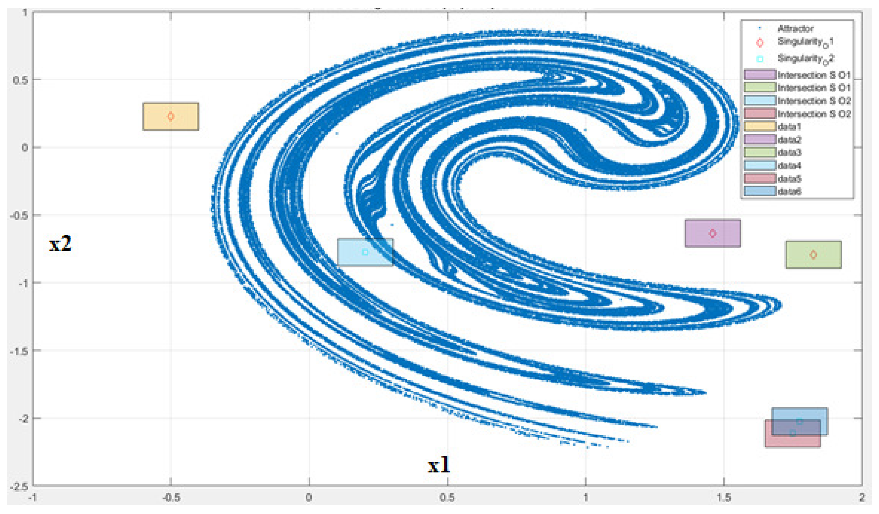
Next, Figure 4 shows in a visual form the overlap between the Clifford system and the singularity manifolds. The belts of different colors are, in theory, lines and are obtained by solving the equations derived from the determinants of the Jacobians calculated above. A 0.2 deviation centered around the theoretical singularity areas/lines was considered in order to find out how many of the experimental attractor points fall into them (the same 0.2 width was used for the other system as well). In this way, an empirical estimation of the overlap between the Clifford attractor and the singularity manifolds was obtained. The red diamonds and the cyan squares are definining the singularity areas/lines for state variables $x_1$ and $x_2$, respectively; $12.26\%$ of the Clifford attractor points overlap with $S_{{\overline{O}}_1}$ and $22.02\%$ overlap with $S_{{\overline{O}}_2}$.

By following a similar approach for the Ikeda map, one can easily obtain the singularity manifolds from (19) and (20):

$$\begin{array}{cc}\hfill S_{{\overline{O}}_1}& =\{(x_1,x_2)\in \mathbb{R}|det\left(O_1\right)=\hfill \\ \hfill & =-u·\left[{\displaystyle \frac{12·[x_2^2·cos\left(t\right)+x_1·x_2·sin\left(t\right)}{{(1+x_1^2+x_2^2)}^2}}+sin\left(t\right)\right]=0\}\hfill \end{array}$$

(19)

$$\begin{array}{cc}\hfill S_{{\overline{O}}_2}& =\{(x_1,x_2)\in \mathbb{R}|det\left(O_2\right)=\hfill \\ \hfill & =-u·\left[{\displaystyle \frac{12·[x_1^2·cos\left(t\right)-x_1·x_2·sin\left(t\right)}{{(1+x_1^2+x_2^2)}^2}}+sin\left(t\right)\right]=0\}\hfill \end{array}$$

(20)

where u and t are defined in (6).

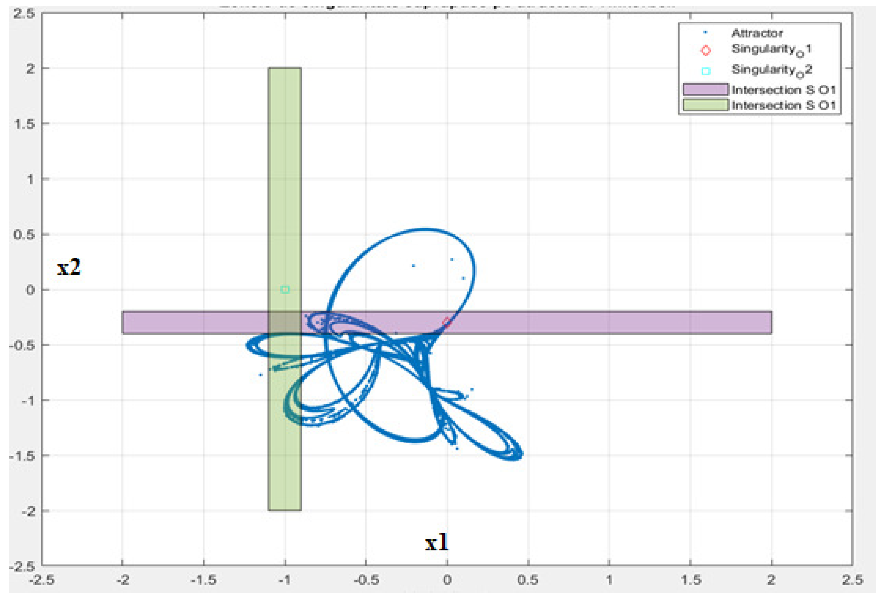
Figure 5 presents the overlap between the Ikeda map and the singularity manifolds. The singularity areas in the attractor region are just dots this time. For reasons of consistency with the Clifford results, an area of 0.2 width around the points was considered in order to evaluate the percentage of overlap between the singularity manifolds and the Ikeda attractor. The red diamonds and the cyan squares are the coordinates of the singularity areas for state variables $x_1$ and $x_2$, respectively; $0\%$ of the Ikeda attractor points overlap with $S_{{\overline{O}}_1}$ and $0.41\%$ overlap with $S_{{\overline{O}}_2}$, much lower figures compared to the Clifford map.

The results for the Tinkerbell map are the easiest to read: one can easily obtain the singularity manifolds from (21) and (22):

$$S_{{\overline{O}}_1}=2·x_2+b$$

(21)

$$S_{{\overline{O}}_2}=-2·x_2-c$$

(22)

where b and c are defined in (7).

Figure 6 presents the overlap between the Tinkerbell map and the singularity manifolds. The singularity areas in the attractor region are again lines, as they were for the Clifford map. For reasons of consistency, the same area of 0.2 width around the lines was considered in order to evaluate the percentage of overlap between the singularity manifolds and the Tinkerbell attractor. The red diamonds and the cyan squares define the coordinates of the lines/singularity areas for state variables $x_1$ and $x_2$, respectively; $2.84\%$ of the Tinkerbell attractor points overlap with $S_{{\overline{O}}_1}$ and $4.83\%$ overlap with $S_{{\overline{O}}_2}$, much lower figures compared to the Clifford map but higher than for the Ikeda map.

The observability and singularity results are combined in a single view in

Table 3. Observability coefficients per state variable and chatic system analyzed.

Chaotic System	${\mathit{\eta }}_1$ Observability Coefficient	${\mathit{\eta }}_2$ Observability Coefficient	Overlap Attractor and ${\mathit{S}}_{{\overline{\mathit{O}}}_1}$	Overlap Attractor and ${\mathit{S}}_{{\overline{\mathit{O}}}_2}$
Clifford	0.54	0.54	12.26%	22.02%
Ikeda	0.17	0.17	0%	0.41%
Tinkerbell	0.44	0.88	2.84%	4.83%

.

3.4. Transient Time and Statistical Independence

The third perspective used to analyze the dynamical systems considered in this paper is the notion of statistical independence. This is an important aspect when judging whether a system is suitable to be used in cryptography and PRNGs. Section 2 describes in detail the theoretical results used to decide if two datasets are statistically independent. The two datasets are extracted from a Monte Carlo simulation for a chosen dynamical system and they are separated by at least the statistical independence distance of the system. There is another important aspect apart from using a big enough time between the moments when the two datasets are selected and that is the transient time. The datasets to be analyzed have to be selected after the transient time elapses. The transient time is a system parameter and is different for each map. It quantifies the moment when the pseudorandom process enters the stationary region.

The Monte Carlo simulation of a generic dynamical system starting with an uniform set of L initial conditions ($x_{i,0}$) is depicted in (23). The term $x_{i,j}^k$ refers to the kth trajectory corresponding to letting the dynamical system run starting from the initial condition $x_{i,0}^k$.

$$M_i=\left(\begin{array}{c}{x}_{i,0}^1{x}_{i,1}^1...x_{i,N}^1\\ x_{i,0}^2{x}_{i,1}^2...x_{i,N}^2\\ .\\ .\\ .\\ x_{i,0}^L{x}_{i,1}^L...x_{i,N}^L\end{array}\right)$$

(23)

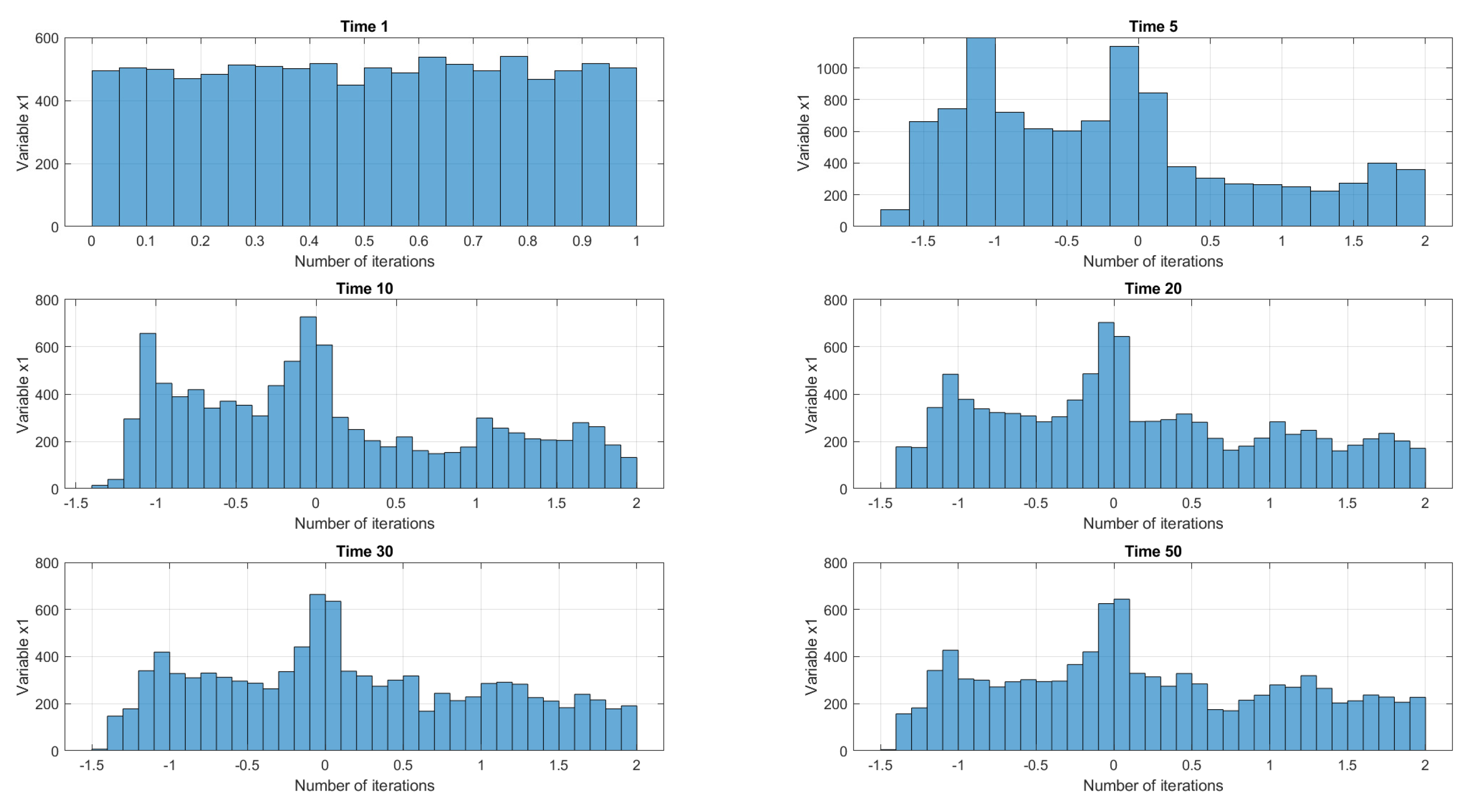
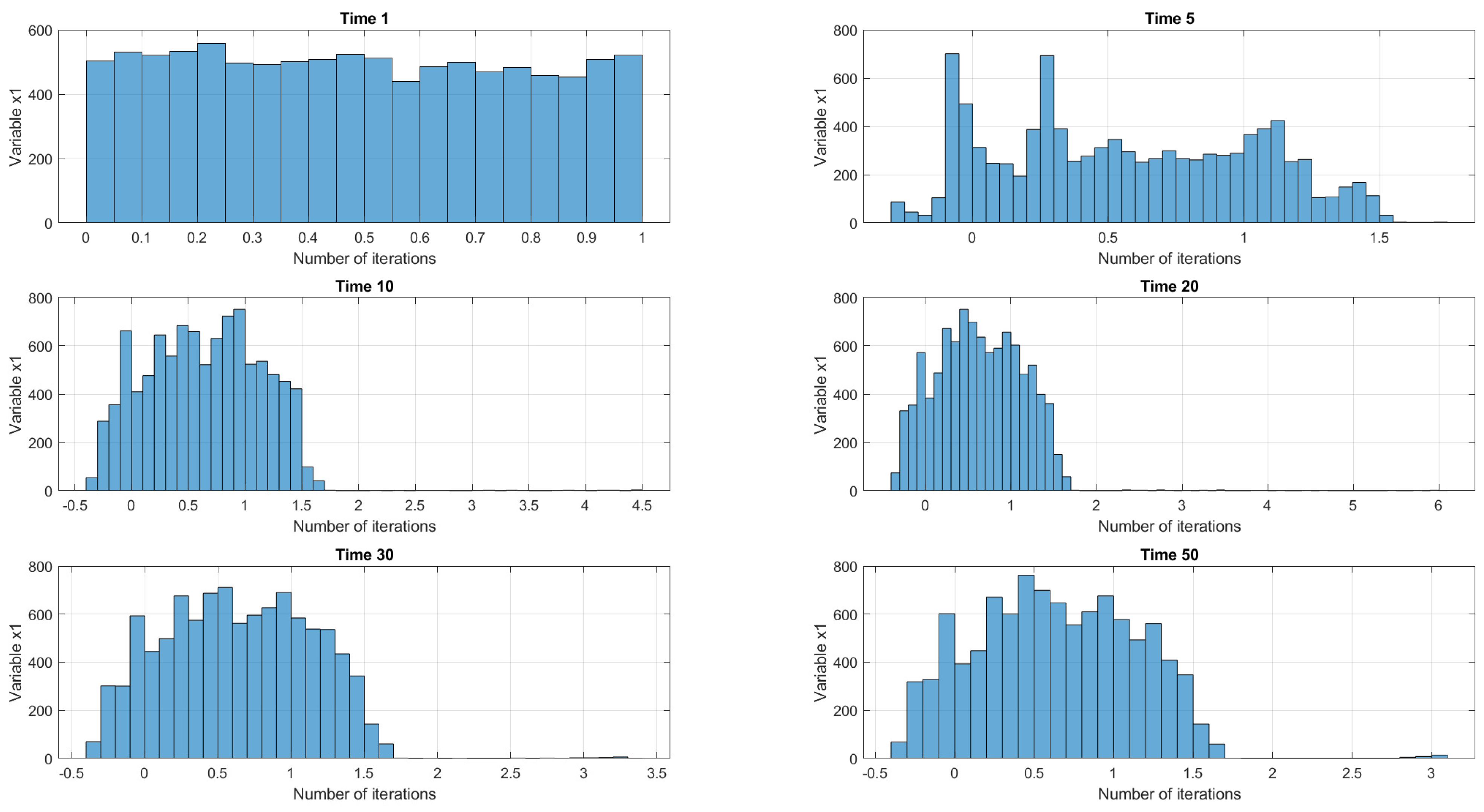
The transient time for the Clifford map is visually depicted in Figure 7. One can easily notice that, at the beginning of the process iteration, the distribution of $x_{1,0}$ is uniform by design (the initial conditions), and as the time goes by ($k\in \{1,5,10,20,30,50\}$), the distribution of values $x_{1,N}^k$ changes to a different one and becomes stable. The transient time for the Clifford system is approximately 30 iterations and, after this moment, the process is stationary. Similar results are obtained for the second state variable $x_2$. It is thus safe to say that the statistical independence distance will be investigated for datasets selected after at least 100 iterations (higher than the transient time), in order to be outside the unstable, non-stationary area of the process.

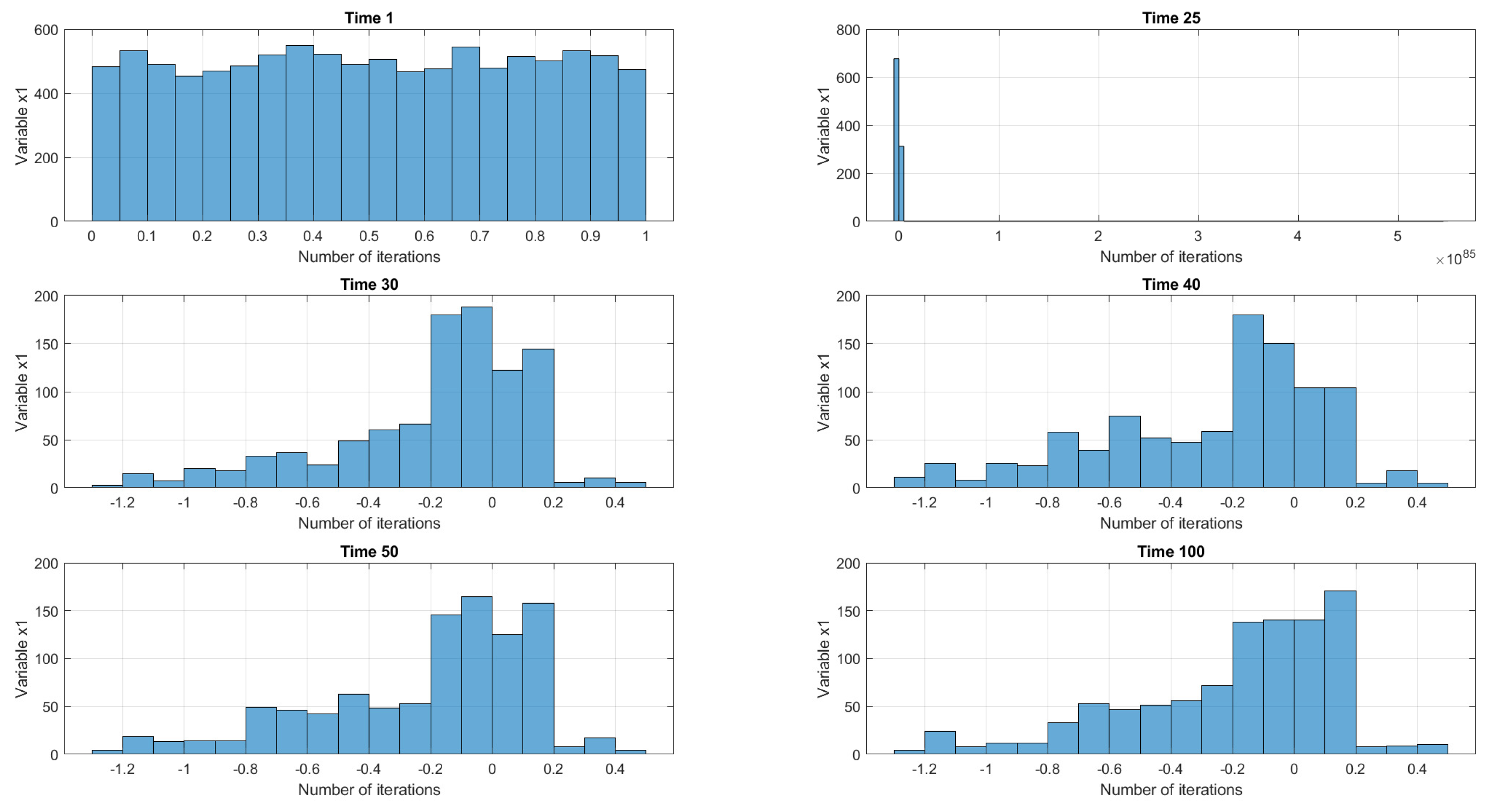
Similar results were obtained for the Tinkerbell (Figure 8) and the Ikeda (Figure 9) maps. What is depicted in the pictures below are the histograms of the $x_1$ variable across multiple iterations obtained via a Monte Carlo simulation at different time moments.

Once the transient time topic is clarified, the next step on the way to find out which of the analyzed systems is suitable to be used as PRNG is to investigate the statistical independence. The statistical independence test described in [18,19] was applied to datasets obtained from the dynamical systems analyzed. The datasets (from iterations $k_1$ and $k_2$) were selected after 100 iterations to be in the stationary area of the chaotic process and were separated by d iterations ($k_2-k_1=d$). State variable $x_1$ was used for the investigation regarding statistical independence, but similar results are obtained when $x_2$ was used instead.

When the statistical independence test passed for a certain minimum d, this was considered the minimum statistical independence distance; any distance higher than d ensured independence as well. Apart from a regular statistical hypotheses test procedure where a test value is compared with a reference value (alpha-quantile) and the test is a Pass or a Fail, the beauty of the Badea–Vlad independence test proposed in [18] is that it allows the researcher to visually evaluate and assess the independence of the datasets in question.

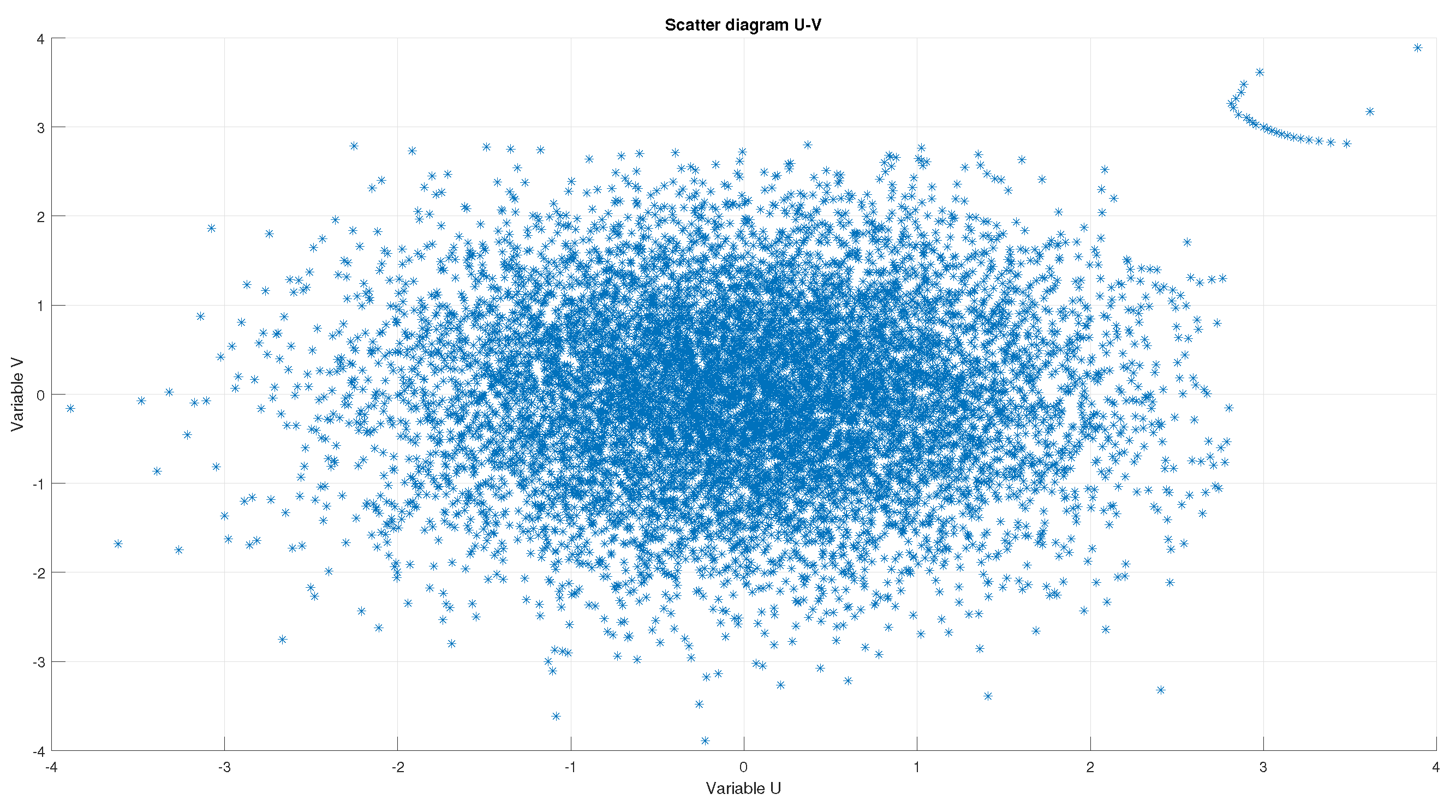
The visual results for the Clifford map are shown in Figure 10. The minimum statistical independence distance for this chaotic system is reasonably low, around 20 iterations. The test procedure passes for any distance higher than the minimum statistical independence distance. The results remain valid independent of the reference $k_1$ iteration where the first data are selected, as long as $k_1$ is higher than the transient time. Visually, the scatter diagrams of the test variables U and V are very similar for $d=20$ and higher. However, for $d=10$, when the test fails, the scatter plot is also much different compared to the joint Gaussian scatter diagram, which is used as a reference, as described in [18,19].

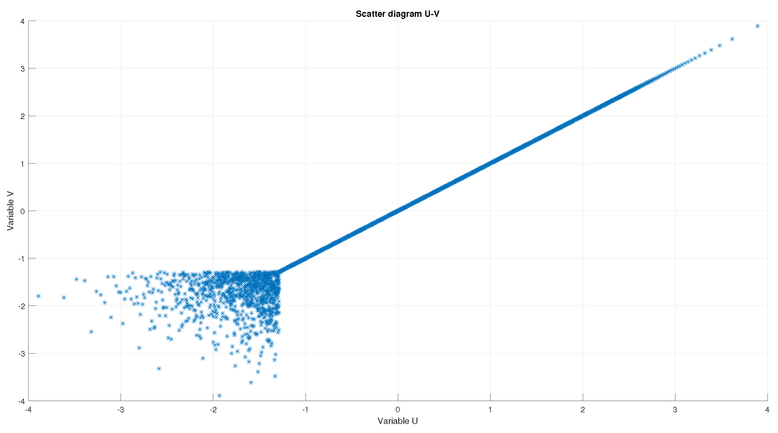
Similar scatter diagrams can be simulated for the Ikeda and Tinkerbell maps. However, these two systems cannot be used to collect independent datasets, as can be seen in Figure 11 and Figure 12. The reason is that the scatter plots do not resemble the one obtained for a jointly bivariate Gaussian variable because there are some clear artifacts linked to data dependency (regular shapes or linear relationships).

4. Conclusions

Taking into account the results presented in Section 3, several important conclusions can be drawn regarding the procedure proposed for the unified testing of different chaotic systems and PRNG selection.

Table 2 shows that there is a correlation between the observability coefficient and the overlap between the attractor and the singularity manifolds (with a slight deviation for state variable $x_2$ for the Tinkerbell map). One can easily notice that the higher the observability coefficient for a specific state variable, the higher the overlap between the singularity region and the attractor of that chaotic system. In practice, systems are chosen such that the overlap is as small as possible because it allows more flexibility during application of data in different cryptographic applications. All in all, from the observability–singularity point of view, out of the three systems analyzed, Ikeda seems the most promising, followed by Tinkerbell and Clifford. Nevertheless, the singularity and observability are not the only concepts that matter. From a statistical independence point of view, as it can be easily noticed in Figure 10, Figure 11 and Figure 12 that the Clifford map is the only one capable of being used as PRNG.

To sum up, this paper presents a novel analysis procedure for dynamical maps, taking into account essential concepts such as statistical independence, singularity, and observability. The great advantage of the thinking flow proposed in this article is that it does not rely entirely on a single notion, no matter how strong that is. Singularity, observability, and statistical independence have been addressed singularly before in the literature, and it is a known fact that they alone can offer important insights into specific problems of interest in cryptography. Nonetheless, making use of the results from all three different perspectives considered together leads to a converged and stronger conclusion that can be used and further investigated from now on by researchers in the field of dynamical systems with cryptographic applications.

The approach proposed can be used for any system, independent of the number of state variables. The experimental results show that there is a fragile equilibrium between the concepts that can be used to select a system for use in cryptography, there is no such concept of one size fits all, and there is more of a compromise that needs to be made by the researcher, depending on the aspect that the respective investigation focuses on.