Article

NARX Deep Convolutional Fuzzy System for Modelling Nonlinear Dynamic Processes

Faculty of Electrical Engineering and Computer Science, University of Maribor, Koroška cesta 46, SI-2000 Maribor, Slovenia
Mathematics 2023, 11(2), 304; https://doi.org/10.3390/math11020304
Submission received: 7 December 2022 / Revised: 25 December 2022 / Accepted: 28 December 2022 / Published: 6 January 2023
(This article belongs to the Special Issue Modeling, Optimization and Control of Industrial Processes)

Abstract

:
This paper presents a new approach for modelling nonlinear dynamic processes (NDP). It is based on a nonlinear autoregressive with exogenous (NARX) inputs model structure and a deep convolutional fuzzy system (DCFS). The DCFS is a hierarchical fuzzy structure, which can overcome the deficiency of general fuzzy systems when facing high dimensional data. For relieving the curse of dimensionality, as well as improving approximation performance of fuzzy models, we propose combining the NARX with the DCFS to provide a good approximation of the complex nonlinear dynamic behavior and a fast-training algorithm with ensured convergence. There are three NARX DCFS structures proposed, and the appropriate training algorithm is adapted. Evaluations were performed on a popular benchmark—Box and Jenkin’s gas furnace data set and the four nonlinear dynamic test systems. The experiments show that the proposed NARX DCFS method can be successfully used to identify nonlinear dynamic systems based on external dynamics structures and nonlinear static approximators.

1. Introduction

Many industrial processes are nonlinear with uncertainty and have time-varying properties. In industrial process modelling, model structure and parameters often change over time. Among the known structural time variations in process plants is the change in the process delay. Obtaining an accurate mathematical model of industrial processes is not an easy task and presents a challenge for system identification. An alternative approach is to develop data-driven (DD) models that do not require a detailed physical understanding of the process and can be extracted from data streams at the same time as data collection. The concept, which assumes the adaptation of both the model structure and the model parameters, is called an evolving system. In [1], an overview of the development of evolving intelligent regression and classification systems is presented, focusing on fuzzy and neuro-fuzzy methods.
In the past, various DD linear model structures have been established, such as state space (SS) models, autoregressive exogenous (ARX) models, Box–Jenkins (BJ) models, and output error (OE) models [2]. These structures can be easily extended to the nonlinear structure, for example, ARX to nonlinear ARX (NARX). However, rule-based (RB) systems, artificial neural networks (ANN) based systems, and a combination of both neuro-fuzzy systems (NFS) can be used to approximate a non-linear static characteristic or an input–output transition function. Fuzzy modelling, as a representative of RB systems, provides fuzzy inference to manage uncertainty and better understand modelling results than ANN or deep learning (DL) methods. It is now well established that fuzzy systems (FS), ANN, and NFS are approximators of all different types of non-linear functions within a compact domain.
In the initial phase of the investigations, linguistic modelling [3] and fuzzy relation equation-based methods [4] were suggested as the basic methods for fuzzy model identification. The Takagi–Sugeno–Kang (TSK) models [5,6,7] have enabled the evolution of more complex rule-based systems where the rules are supported by local regression models. TSK training algorithms are characterised by a division into separate model structure identification and parameter estimation, where structure identification is assumed to be the determination of the number of rules and the parameters of the membership functions of the fuzzy sets in the rules. On the consequent side of the rules are the parameters of the linear models, which are usually determined by the least squares method. Later, researchers started to pay attention to the integration of a non-linear autoregressive model with exogenous input (NARX) into an intelligent model [8,9,10,11,12]. Intelligent models with NARX structure have good predictive properties, and they are widely used for the modelling and identification of nonlinear dynamical systems [13]. Paper [14] reviews hybrid models that combine the advantages of FS and ANN using training algorithms based on supervised learning methods. When modelling complex non-linear systems, these methods have the disadvantage of a large rule base with many rules. Rule generation is complex and often not understandable. In the case of a large training dataset, it is difficult to process it efficiently with iterative learning algorithms, which are characterised by multiple passes over the same pieces of data.
The applicability of FS or NFS is limited by the number of input variables and the number of fuzzy sets defined on the domains of the input and output variables. Increasing these numbers leads to a problem known in the literature as the “curse of high dimensionality”. Researchers have proposed some feature reduction approaches to be used before applying the training algorithm. In our early work [15], we addressed this problem by proposing a method to decompose a single large FS into smaller subsystems. By following the decomposition mechanism of the fuzzy inference procedure, we have applied several simple single-input-single-output (SISO) decomposed fuzzy inference systems (FIS) to model dynamic systems. The proposed decomposition was based on a FS represented by a fuzzy relational equation. In order to improve the performance we later presented the structure of a decomposed NFS ARX model [16] for modelling unknown dynamical systems.
Today, we are dealing with a huge amount of data and many features when modelling complex dynamic processes. As a result, the performance of traditional neuro-fuzzy classification and prediction systems is reduced. A hierarchical fuzzy system (HFS), first proposed by Raju et al. [17], shows better performance than general FS for big data prediction [18,19,20,21,22]. The training algorithms for HFS are mostly of the same types as those for ANN or deep convolutional neural networks (DCNN) [23]. Those algorithms are mainly iterative in their nature and, therefore, they are computationally intensive when applied to problems with a huge amount of data and many features. The deep convolutional fuzzy system (DCFS), proposed in [24], is a hierarchical fuzzy structure, which can overcome the deficiency of general FS when facing high dimensional data. The DCFS hierarchical structure has the form of a pyramid made up of several smaller simple fuzzy subsystems (FSs). A high dimensional data set input into the DCFS is split into several small datasets and delivered to FSs in the first structure layer. The first layer FSs are designed using the WM training method [25,26] and may be represented as the ordinary week estimators [25]. By passing the training data through FSs of the first level, a data set for the second level is generated, and the training procedure may be repeated.
In this paper, we propose to use DCFS as approximators of unknown nonlinear functions, in the NARX structure, to model nonlinear dynamic processes (NDPs). We investigated the significance of the appropriate selection of the structure of the FSs at the first level of the DCFS. We test the proper FSs input–output signal selection at the first level of the DCFS, which has an impact on the final approximation properties. An important result is the definition of three different NARX DCFS structures. For the proposed NARX DCFS, we have adapted the WM algorithm to be suitable for training on the input/output data of different processes.
This paper consists of five sections. In Section 2, we present the basics of nonlinear dynamic input/output modelling with an external dynamic’s principle, the concept and implementation of the Wang–Mendel FS, and the idea of the DCFS. We continue by presenting the main contribution of the research, which is the adaptation of the DCFS for modelling the nonlinear static approximators of the nonlinear time-invariant dynamic systems. There are three different NARX DCFS structures proposed, and the training algorithm is adapted. Section 3 presents the experimental results tested on different data sets to validate the proposed method. The modelling results are evaluated and are analysed in Section 4, where we summarise the strengths and weaknesses of the proposed modelling method. Finally, the last section concludes the paper.

2. Materials and Methods

In this section, we will give details on how to apply a NARX DCFS for nonlinear system modelling. The non-linear behaviour of time-varying dynamical systems is often modelled by approximating static non-linearities in combination with linear dynamical systems. Such models are used to predict the output of a process, which can either be one-step or long-term predictions. In the case of one-step forecasting, a nonlinear static function approximator (NSFA) is used to predict the output of the model based on the past inputs and outputs of the process. Such a model is often used in predictive and adaptive control systems. Alternatively, a NSFA can be used to predict the output of a process over a long-time horizon, in which case a multi-step prediction with a longer prediction horizon is performed.
In the following subsections, we present models, methods, and notations needed to implement and understand the proposed NARX DCFS model and its application for modelling NDPs.

2.1. Nonlinear Dynamic Input/Output Models Based on External Dynamics

A nonlinear SISO system in the continuous time space is defined as
y ( t ) = H ( u ( t ) )
where u ( t ) ,   y ( t ) R are the input variable and output variable, and H ( t ) is a bounded continuous nonlinear function. By performing discretization with sampling time T s ,   t = k · T s , a discrete-time SISO nonlinear system is given as follows
y ( k ) = f ( y ( k 1 ) , y ( k n y ) , u ( k τ 1 ) , u ( k τ n u ) )
where u ( k ) and y ( k ) are the system input and output at a discrete time k , respectively,   n u and n y are the discrete lags for the input and output signals depending on the unknown system orders, τ is a delay, and f ( · ) is an unknown nonlinear function.
The external dynamics (ES) strategy is a popular and widely used structure for nonlinear dynamic system (NDS) modelling. ES means that the nonlinear dynamic model can be divided into two parts: a static approximator of the nonlinear function and a delay mechanism for the input and output signals, as shown in Figure 1.
The structure in the Figure 1 is also well known from linear dynamic models. Most nonlinear dynamic input/output models can be expressed in the following form:
y ^ ( k ) = f ( φ ( k ) )
where φ ( k ) is a regression vector that may include the prior and, optionally, the actual input process data, the previous output process (or model) data, and the prior prediction errors. e ( k i ) ,   i = 1 , 2 n y . By choosing a regression vector, we choose a structure familiar from linear dynamic models. If we only have lagged outputs in the regression vector, then we model nonlinear time series (NTS). Other popular nonlinear input/output models are summarised in Table 1.
Note that, when modelling NDPs, complexity usually increases significantly as the dimensionality of the input space increases. This is the reason why lower dimensionality models—NTS, NARX, and OE—are more widespread.
Over the last three decades, regression techniques, as well as ANN, FIS, and ANFIS [27], have been widely employed for modelling the nonlinear static approximators of the nonlinear time-invariant dynamic systems. ANNs allow accurate predictions, but the resulting model structures are not useful for explaining the physical background of the process being modelled. FSs and NFSs are inherently better suited for interpreting physical behaviour, as their properties are usually described by if-then rules. A simple FS and a corresponding DD learning method, called the Wang–Mendel (WM) method, proposed in [25], was one of the first methods to model FSs from data and is still a strong and applicable method for DD learning. As WM is the FS used in DCFS, we describe it, in detail, in the next subsection.

2.2. WM Fuzzy System

The WM fuzzy system is standard FS designed with fuzzy rules. Following fuzzy IF-THEN rules allow for modelling the behaviour of the output variable y depending on the input variables x = ( x 1 ,   , x n   ) T :
IF   x 1   is   A 1 ( q )   and and   x m   is   A m ( q )   THEN   y   is   B ( q )
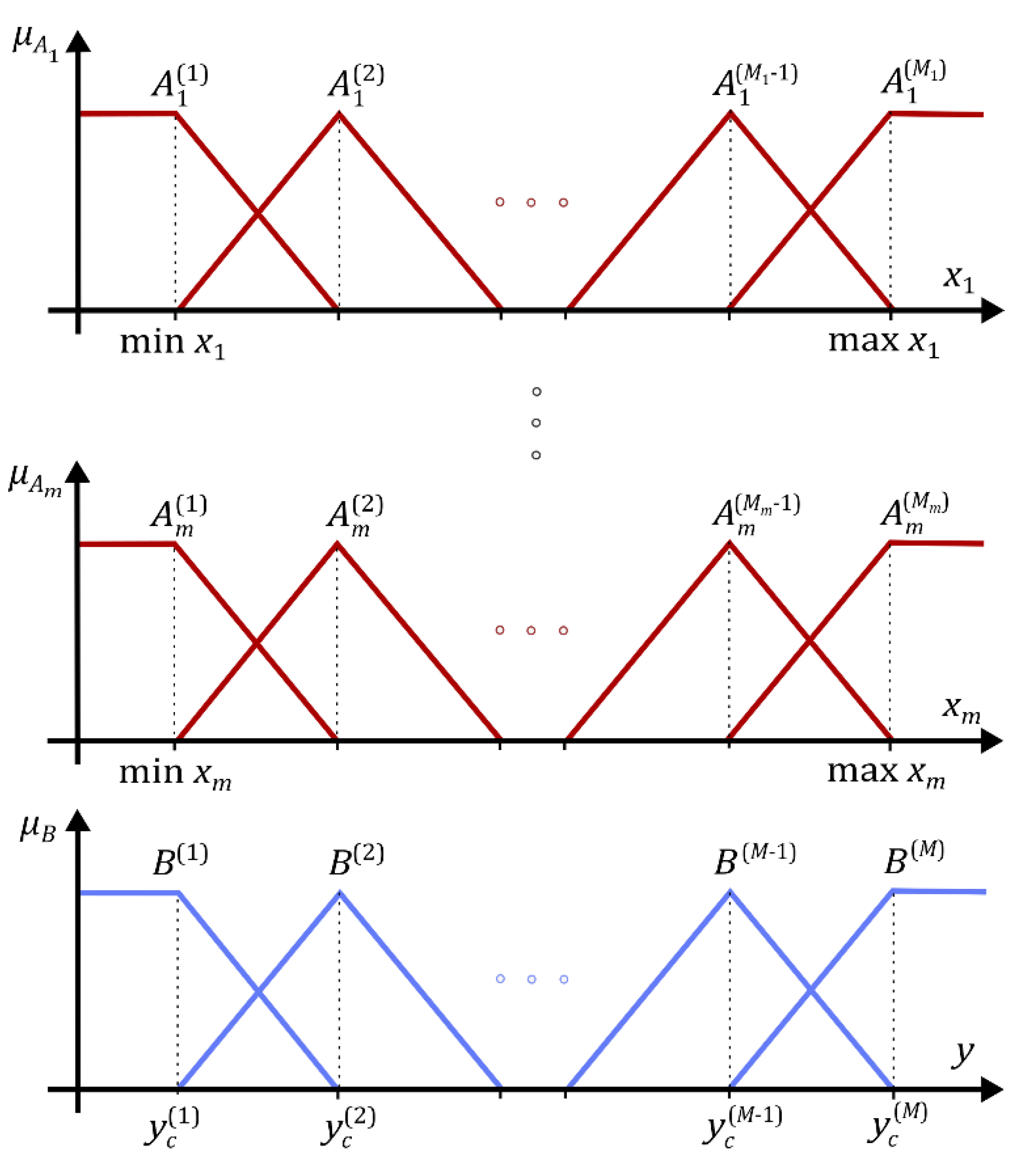
where A j ( q ) and B ( q ) are fuzzy sets defined in rule base R, q is the index of the rule, and ( j = 1 , , m   ) is a subset of ( 1 , , n   ) . The selection of the m input variables in (4) with m n means that the rules can consist of a limited selection of input variables. Fuzzy sets A j ( q ) and B ( q ) are defined as shown in Figure 2, where the centers of the fuzzy sets are equidistant between min   x j and max   x j . For simplicity, assume that M 1 = M j = M m in the following notation. Therefore, the maximum number of rules is M = M i m .
A fuzzy inference mechanism aggregates the rules from a fuzzy rule base into a mapping from fuzzy input set A in the input space R m to fuzzy set B in the output space R . The fuzzifier f u z z ( x ) converts the crisp input x , into the fuzzy set A , and the defuzzifier d e f u z z ( B ) determines a crisp single point y in the output space R that best represents the fuzzy set B . For fuzzy reasoning, the product fuzzy inference mechanism is
μ B ( y ) = max q = 1 , M { sup x R m   [ μ A ( x ) j = 1 m μ A j ( q ) ( x j ) μ B ( q ) ( y ) ] } ,
where m is number of inputs x i 1 ,   , x i m we used following singleton fuzzifier
μ A ( x ) = f u z z ( x ) = { 1 ,   if   x = x 0 ,   otherwise
and center–average defuzzifier
y = d e f u z z ( B ) = q = 1 M y c ( q ) ( j = 1 m μ A j ( q ) ( x j ) ) q = 1 M ( j = 1 m μ A j ( q ) ( x j ) ) ,
where y c ( q ) are the midpoints of the symmetric triangular membership functions of the output fuzzy sets B ( q ) . Note that, for the membership functions presented in Figure 2, we simplify the expression by recognizing that q = 1 M ( j = 1 m μ A j ( q ) ( x j ) ) = 1 , and the denominator of the FS (7) is equal to 1, and FS is simplified to
y = q = 1 M y c ( q ) ( j = 1 m μ A j ( q ) ( x j ) ) .
Note that the FS (8) is considered from the M fuzzy rules (4), with each rule covering a cell ( j 1 , , j m   ) in the m dimensional input space, which means that FS implements local inference with one rule representing one input–output relationship. As a result, this relationship can be represented by the parameter y c ( q ) .
The mapping of the non-linear function of the dynamical system (3) is created using only the information, which is written into the appropriate regression vector depending on the structure of the chosen nonlinear input/output model from Table 1. The inputs to the FS (8) for modelling a nonlinear static approximator are, therefore, x ( k ) = φ ( k ) and the dimension of the input vector can be quite large. Both FSs and non-FSs methods based on fuzzy rules (4) are characterised by the problem of the curse of dimensionality. This means that, in the case of many input variables m and a large number of fuzzy sets, M i of fuzzy sets per input variable greatly increases the number of rules M . In our previous research [28], the problem of too many fuzzy rules to model more complex dynamical systems was solved by decomposing the FS into several simple FSs with fewer input variables. The principle is based on the decomposition of the inference mechanism. As an example, the approximation of the nonlinear function with the decomposed FS having n u + n y input variables would be replaced by n u + n y FSs with one input and one output, as well as with two-dimensional fuzzy relations R i . The output of the simplified decomposed fuzzy model is
y = 1 n u + n y · { d e f u z z [ f u z z ( u ( k τ 1 ) ) ° R b 1 ] + + d e f u z z [ f u z z ( u ( k τ n u ) ) ° R b n u ] + d e f u z z [ f u z z ( y ( k 1 ) ) ° R a 1 ] + + d e f u z z [ f u z z ( y ( k n y ) ) ° R a n y ] } ,
where ° represents a set of composition operators (i.e., max–min, max–prod, sum–prod, etc.) and R is the relational matrix. The structure of the dynamical system (9) used to model the non-linear process is like that of the discrete linear ARX model. The difference is that the linear parameters a i and b i of the linear ARX model are substituted with simple FSs. In [16], we analyze the advantages of this approach and outline the drawbacks. Advantages of the simplified decomposed fuzzy model are fewer rules in rule base; two-dimensional fuzzy relations; code optimization and hardware inference realization are possible; similarity between the structure of the suggested model and the discrete linear ARX model. However, the analysis of the results also showed certain weaknesses resulting from the decomposition of a FS into several simple ones. In the case of approximation of complex nonlinear dynamic function, the trained model is worse at predicting the output of the process than in the case of an undecomposed FS. We have concluded that simplifying the structure of a FS into several simple FSs connected at a single level brings limitations in the approximation of complex non-linear functions. We started to look for a solution in the multilevel connection of simple FSs, which led us to study the hierarchical FSs, which include DCFS.

2.3. Deep Convolutional Fuzzy System

The key idea behind deep modelling is mostly in the multi-layer nature of the method, the transformation of features in the model, and the sufficient complexity of the model. DCFS, proposed in [24], represents a new principle of development—a hierarchical FS based on the WM method—in particular, for high-dimensional mappings. The DCFS is based on the use of the WM method of learning from data to determine simple multilevel multidimensional FSs. The design proceeds from lower levels to higher levels using the WM method [25,26]. The number of inputs of simple FSs is determined by a so-called moving window, which acts as a convolution operator.
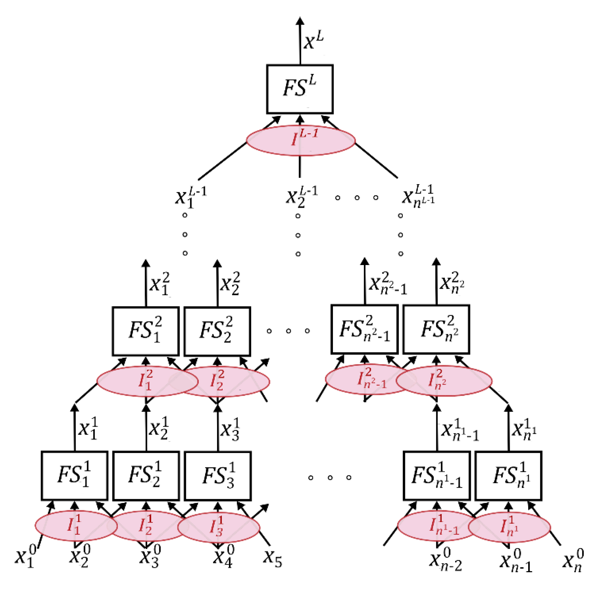
In [24], DCFS was developed for stock index prediction. The structure of the DCFS is presented in Figure 3. The DCFS contains n inputs mapped to the input vector ( x 1 0 , x 2 0 , , x n 0 ) , and the scalar output x L . Level l   ( l = 1 ,   2 ,     , L 1 )   is composed of n l fuzzy systems F S i l   ( i = 1 ,   2 ,     , n l ) , the outputs of which are marked as x i l , and represents inputs to higher level l + 1 FSs. At the last level, there is only one F S L , which processes the n L 1 outputs from level L 1 and gives the final DCFS output x L . The fuzzy systems F S 1 l ,   F S 2 l ,   , F S n l l   ( l = 1 ,   2 ,     , L 1 ) and their inputs were obtained as outputs from the lower level F S i l 1 outputs x 1 l 1 , x 2 l 1 , , x n l 1 l 1 . Those using a moving window are grouped into the input sets I 1 l , I 2 l , , I n l l . The purpose of the moving window is to determine the number of FSs in the layers and the number of inputs to a particular F S i l . It performs a double task. Namely, it determines the size m l of the moving window, and it determines the moving pattern, which refers to the number of inputs that are moved in each step.
.
The choice of the length m of the moving window is important and can be different for F S i l at different levels. The number should not be too large, as this will lose the advantages of DCFS over a conventional FS. At the same time, it should not be too small. It is usually chosen between 2, 3, 4, or 5, and it may move one input at a time or more than one input at a time to cover all variables in the level. The strategy of moving inputs to individual F S i l can also be changed. This provides a variety of DCFS structure options.
In [24], the author argues that the DCFS learned from the data with the WM learning method has a better model interpretation capability compared to the DCNN results. The WM training method determines the parameters y c ( l ) , l = 1 ,   2 , , M of the FS (8), which is used for all F S i l ( i = 1 ,   2 , , n l ) and ( l = 1 ,   2 , , L 1 ) in the DCFS. Details on the adaptation of the WM training method [26] for DCFS training are detailed in [24].
In next section, we will give details on how to apply a DCFS for system modelling of the nonlinear dynamic input/output models based on a nonlinear static approximator and an external tapped delay line.

2.4. Nonlinear Dynamic Input/Output Models Based NARX DCFS

The main contribution of this research is the adaptation of DCFS for modelling the nonlinear static approximators of the nonlinear time-invariant dynamic systems, which are based on ED structures, such as the NARX structure. First, it is necessary to investigate the appropriate structure of the DCFS input vector fitted to the input regression vector of the NARX structure (Table 1). There are many possibilities, but several structures make more sense, which we describe below.

2.4.1. Different NARX DCFS Structures

NARX DCFS structures differ in the number of l, (l = 1, 2,     ,   L) hierarchical levels of the DCFS, the number of nl fuzzy subsystems F S i l in each level, the selection and number of inputs to the fuzzy subsystems (moving window I i l ), and the way in which all the fuzzy subsystems are implemented. The fuzzy subsystems F S i l are defined by the number of inputs, as well as the number of fuzzy sets on the input and output variables. The FSs may be equal at all levels, or they may be different. In the following, we assume the same number M = M 1 = M m of fuzzy sets on the inputs and outputs of all fuzzy subsystems F S i l .
First, let’s start by defining the general structure of the order n.
Definition 1.
The General NARX DCFS structure of the order nu, ny maps the input regression vector  φ ( k ) = [ y ( k 1 ) , y ( k n y ) , u ( k τ 1 ) , u ( k τ n u ) ] directly to the DCFS input vector  ( x 1 0 , x 2 0 , , x n 0 ) , where n = nu + ny, and τ is a dead-time. The input sets  I 1 l , I 2 l , , I n l l to the fuzzy systems  F S 1 l ,   F S 2 l ,   , F S n l l   (l = 1, 2,   , L 1 ) are selected from the previous level’s outputs  x 1 l 1 , x 2 l 1 , , x n l 1 l 1 using a moving window of the length m with moving scheme where it may move one variable at a time starting from  x 1 l 1   until  x n l 1 l 1 .
Note that the general NARX DCFS has FSs in the first level where the inputs in the moving window I 1 1 , I 2 1 , , I n 1 1 are not arranged according to any rule. The inputs are ordered sequentially, as they are written in the regression vector. An example of general NARX DCFS with nu = 3, ny = 3, n1 = 4, m 1 = m 2 = 3 ,   m 3 = 2 , and L = 3 is presented in Figure 4a. When selecting the inputs for the F S i 1 at the first level, it is reasonable to select the inputs from the regressor vector φ ( k ) in a way that makes sense. The next NARX DCFS structure choice is based on combining the delayed inputs u ( k τ 1 ) , u ( k τ n u ) together as inputs for the moving windows of the first half of F S i 1 at the first level. Similarly, the combined delayed outputs y ( k 1 ) , y ( k n y ) of the regression vector are inputs for the second half of F S i 1 at the first level. This principle can be continued at higher levels up to the last level. Due to the division of FSs into input and output parts, we called this structure the Input-output NARX DCFS structure.
Definition 2.
The Input-output NARX DCFS structure of the order nu, ny maps the input regression vector  φ ( k ) = [ y ( k 1 ) , y ( k n y ) , u ( k τ 1 ) , u ( k τ n u ) ] to the DCFS input vector  ( x 1 0 , x 2 0 , , x n 0 ) , where n = nu + ny, and τ is a dead-time. At the first level, FSs are divided into input part consisting of  F S u i 1 with the moving windows  I u i 1 which contain input regressors u ( k τ 1 ) , u ( k τ n u ) , and output part consisting of  F S y i 1 with the moving windows  I y i 1 which contain input regressors  y ( k 1 ) , y ( k n y ) .
An example of input–output NARX DCFS with nu = 3, ny = 3, n1 = 4, m1 = 2, m2 = 3, m3 = 2, and L = 3 is presented in Figure 4b. The first two FSs at the first level, F S 1 1 and F S 2 1 , process delayed inputs, and the second two, F S 3 1 and F S 4 1 , process delayed outputs.
The next option for selecting the inputs for the F S i 1 at the first level, which is frequently used in hierarchical FSs-based dynamical models, is the selection of lower-order dynamic sub-models.
Definition 3.
The Sub-model NARX DCFS structure of the order nu, ny maps the input regression vector  φ ( k ) = [ y ( k 1 ) , y ( k n y ) , u ( k τ 1 ) , u ( k τ n u ) ] to the DCFS input vector  ( x 1 0 , x 2 0 , , x n 0 ) , where n = nu + ny, and τ is a dead-time. At the first level, FSs are organized as lower order sub-models with the moving windows I i 1 which contain input regressors  u ( k τ i ) , u ( k τ i n u i 1 ) , y ( k i ) , y ( k i n y i 1 ) , where  n u i 1 n u   and  n y i 1 n y are lags for the output and input signals if sub-models.
An example of input–output NARX DCFS with nu = 3, ny = 3, n1 = 3, n u 1 1 = n u 2 1 = n u 3 1 = 1 , n y 1 1 = n y 2 1 = n y 3 1 = 1 , m 1 = m 2 = m 3 = 2 , and L = 3 is presented in Figure 4c. We see that, at the first level, we have three FSs that approximate the dynamic behaviour of the first order. Similarly, we could have higher-order systems. Structures of each of the FSs are not necessarily always the same, and the possibilities are almost unlimited.
Remark 1.
With the proper selection of parameters, practically any FS may be presented as a DCFS. The selection of parameters l = 1, n1 = nu + ny, m1 = nu + ny fuzzy subsystem  F S 1 1 gives a structure which is the same as general fuzzy system (GFS) based on the ARX model structure presented in [4]. In a similar way, the choice of parameters l = L, n1 = nu + ny, m1 = 1, ml = 2,  l = 2 , 3 L can be combined to give a structure like the simple decomposed fuzzy ARX model of the SISO dynamic system (9) proposed in detail in reference [16]. Instead of a multi-level structure, the outputs of the first level can be averaged, resulting in exactly same structure.
The system identification procedure of a nonlinear dynamic input–output model involves constructing an appropriate model from input–output data. In the next subsection, we present a training algorithm that enables fast parameter training of F S i l based on input–output data.

2.5. Fast Training Algorithm for NARX DCFS Structures

The main training algorithm of DCFS is the Wang–Mendel (WM) method [25,26]. The original MATLAB code of the DCFS training algorithm [24] is published in a text file at: https://ieeexplore.ieee.org/ielx7/91/9130783/8788632/code_training_algorithm.pdf?arnumber=8788632&tag=1, accessed on 27 December 2022.
We have adapted the training algorithm code to the proposed NARX DCFS structures. It is not an iterative method; rather, it is based on a rule extraction approach from data. Given the N input–output data pairs u ( k ) ,   y ( k ) , k = 1 , 2 N , where y ( k ) and u ( k ) are the at time k , the task of the training algorithm is to design a NARX DCFS parameter to match this input–output pair. The training method for DCFS proposed in [24] has been modified to allow effective training of the NARX DCFS structures. We continue with the description of the extended training method, which we present as an Algorithem 1, as follows.
Algorithm 1
Step 1. Choose the structure of the NARX DCFS.
     Define the n y , n u , τ of regression vector φ ( k ) = [ y ( k 1 ) , y ( k n y ) , u ( k τ 1 ) , u ( k τ n u ) ] .
     Define the NARX DCFS structure and the way the NARX regression vector φ ( k ) is mapped to the DCFS input vector ( x 1 0 , x 2 0 , , x n 0 ) .
     Create data pair for DCFS training [ x 1 0 ( k ) , , x n 0 ( k ) ;   y 0 ( k ) ] ,   k = 1 , 2 N .
Step 2. Choose the structure of the DCFS.
     Define the number hierarchical levels of the DCFS of L, the number of nl fuzzy subsystems F S i l in each level, and the number of inputs to the fuzzy subsystems m l , l = 1 , 2 L (moving window I i l ).
     Choose the moving scheme I i l .
     Choose the number M of fuzzy sets for all inputs and all F S s .
Step 3. Design the first level F S i 1 (i = 1, 2,   , n 1 ) in the form of (8), using the WM method [24,25,26], where the data pairs are [ x i 0 ( k ) , , x m + i 1 0 ( k ) ;   y 0 ( k ) ] ,   k = 1 , 2 N .
    Step 3.1. For each cell ( j 1 ,   j 2 , , j m ) with j 1 ,   j 2 , , j m = 1 , 2 , , M set the initial values of the weight parameter w j 1 , , j m and the weight output parameter u j 1 , , j m equal to zero.
    Step 3.2. For each input x i 0 , , x i + m 1 0 to F S i 1 , consider the M fuzzy sets A 1 ,   , A M , with membership functions of triangular shape, symmetrically arranged as in the Figure 2, and choose the endpoints as
min   x i 0 = min ( x i 0 ( k ) | k = 1 , 2 N ) max   x i 0 = max ( x i 0 ( k ) | k = 1 , 2 N ) min   x m + i 1 0 = min ( x m + i 1 0 ( k ) | k = 1 , 2 N ) max   x m + i 1 0 = max ( x m + i 1 0 ( k ) | k = 1 , 2 N ) (10)
    Step 3.3. For each data pair [ x i 0 ( k ) , , x m + i 1 0 ( k ) ;   y 0 ( k ) ] ,   k = 1 , 2 , , N determine the fuzzy sets A j 1 * ,   , A j m * that achieve the maximum membership values among the M fuzzy sets A 1 ,   , A M at x i 0 ( k ) , , x i + m 1 0 ( k ) . Determine
j 1 * = arg   max j { 1 , 2 , M } ( A j ( x i 0 ( k ) )   ) j m * = arg   max j { 1 , 2 , M } ( A j ( x m + i 1 0 ( k ) )   ) (11)
    Step 3.4. Update the weight parameters w j 1 * ,   , j m * and weight output parameters u j 1 * ,   , j m * for cell j 1 * ,   , j m *
w j 1 * ,   , j m * = w j 1 * ,   , j m * + A j 1 * ( x i 0 ( k ) )   A j m * ( x m + i 1 0 ( k ) ) u j 1 * ,   , j m * = u j 1 * ,   , j m * + ( A j 1 * ( x i 0 ( k ) )   A j m * ( x m + i 1 0 ( k ) ) ) · y 0 ( k ) (12)
    Step 3.5. Repeat Steps 3.3 and 3.4 for k = 1 , 2 N . For the cells ( j 1 , , j m ) with w j 1 , , j m 0 , determine the parameters y c j 1 , , j m in the F S i 1 of (8) as
y c j 1 , , j m = u c j 1 , , j m w c j 1 , , j m .(13)
        Cells ( j 1 , , j m ) with w j 1 , , j m 0 are covered by data, and define
Y c ( 0 ) = { ( j 1 , , j m )   | ( j 1 , , j m )   where   is   w j 1 , , j m 0   } .(14)
    Step 3.6. For each cell ( j 1 , , j m ) not in Y c ( 0 ) , search its neighbors to see whether they are in Y c ( 0 ) , where two cells, ( j 1 , , j m ) and ( j 1 , , j m ) , are neighbours to each other if j i = j i for all i = 1 , 2 , , m except at one location r, such that the j r = j r + 1 or j r = j r 1 . For the cells ( j 1 , , j m ) not in Y c ( 0 ) that have at least one neighbor in Y c ( 0 ) , determine the y c j 1 , , j m as the average of the y c j 1 , , j m ’s of its neighbors in Y c ( 0 ) . Define
Y c ( 1 ) = Y c ( 0 )     { ( j 1 , , j m )   |   y c j 1 , , j m   is   determined   in   this   step } (15)
    Step 3.7. Repeat Step 3.6 with Y c ( 0 ) replaced by Y c ( 1 ) , and Y c ( 1 ) replaced by Y c ( 2 ) , and continue this process to get Y c ( 3 ) ,   Y c ( 4 ) , , Y c ( p ) that contain the cells ( j 1 , , j m ) with j 1 , , j m =   1 , 2 , , M . For more features of the Wang–Mendel (WM) method and a detailed description, refer to [25,26].
Step 4. Repeat Step 2 for l = 2 up to L, designing the FSs at all levels. For example, for level l we design the s F S i l , i = 1 , 2 , , n l , assuming that, in the previous step, we have designed all FSs from level l-1.
    Step 4.1. For each k = 1 , 2 N put x 1 0 ( k ) , x 2 0 ( k ) , , x n 0 ( k ) input to DCFS level 1 and compute upwards along the DCFS to get the outputs of level l-1. The outputs of FSs of level l-1 are denoted by x 1 l 1 ( k ) , x 2 l 1 ( k ) , , x n l 1 l 1 ( k ) . We create new input–output data pairs [ x 1 l 1 ( k ) , x 2 l 1 ( k ) , , x n l 1 l 1 ( k ) ,   y 0 ( k ) ] ,     k = 1 , 2 N for designing the level l  F S i l .
    Step 4.2. Repeat Step 3, and train the level l  F S i l , i = 1 , 2 , , n l with the new input–output data pairs [ x 1 l 1 ( k ) , x 2 l 1 ( k ) , , x n l 1 l 1 ( k ) ,   y 0 ( k ) ] , with k = 1,2⋯N.
    Step 4.3. Set the l = l +1 and repeat Steps 4.1 and 4.2 until the last F S L on the level L is designed.
Note that the proposed training algorithm is much faster than the standard gradient descent-based algorithms, such as back propagation (BP). All the F S i l in the DCFS are designed with N data, which are applied once in the training procedure, rather than iteratively several times, as is necessary for gradient-based and other iterative learning methods. In the following, we present the proposed NARX DCFS structure for the prediction of nonlinear dynamical systems.

3. Experimental Studies

With the aim of evaluating the applicability of the NARX DCFS for modelling non-linear dynamic systems, all three structures defined in Section 2.4.1 were tested on different sets of benchmark test data in ordering, gas furnace system input–output modelling, and several nonlinear dynamic test processes. All experiments were performed in MATLAB R2021b on a PC with Intel® Core™ i7 CPU 870 @ 2.93 GHz 2.93 GHz and Windows 10 Pro operating system. The program code for all experiments in the study and the necessary data sets are available as Supplemental Material.

3.1. Gas Furnace Model Identification

We selected Box and Jenkin’s benchmark [29] to test, analyse, and validate the modelling results. The data in this dataset were obtained as measurements from the combustion process in an industrial furnace. The input data is the methane flow rate, while the output data is the CO2 concentration in the combustion gases. The modelling data represent 296 measurements that were sampled with a sampling time of 9s. The modelling objective is to predict y(k) at a fixed iteration k based on the available knowledge of the behaviour of the system at previous time instances. The objective of the modelling is to predict the output based on the past input–output data and, since it is a dynamic system, a regression vector of appropriate dimensions and with appropriate delay is first chosen. The new y(k) is affected by the following input–output variables [y(k-1), ⋯y(k-ny), u(k- τ -1), ⋯u(k- τ -nu)]. In the above examples, n u = 3 and n y = 3 were chosen, and the delay τ was varied between 1 and 4.
For comparing the quality of performance, a mean square error (MSE) was chosen as a measure of the prediction quality
M S E = 1 N τ n u + 1 k = τ + n u   N [ y ( k ) y ^ ( k ) ] 2
Calculating the MSE of the output variable tells us what the average estimation error of our model is. For example, M S E = 0.5 represents an average estimation error of about 1.3 % . From this, we conclude that the M S E 0.5 values for this benchmark are already a reasonably good result. In this study, we take the MSE index as a measure to compare the output prediction results of different fuzzy models against the predictions of the proposed NARX DCFS model structures.
In our first experiment, we used a WM FS (7) proposed and the WM system identification method. When modelling with FSs, some standard steps must be implemented at the start, such as the choice of the number of fuzzy sets M on each input and output variable, the shape of the membership functions, and the placement of these fuzzy sets on the definition ranges of the input and output variables. Triangular shapes of the membership functions, which were placed symmetrically to equally cover the entire definition ranges of the variables, were chosen. Another important step in modelling dynamical systems is the correct choice of the delay τ and orders nu, ny, of the system, which have important impacts on the structure of the regressor vector that is the input to the FS. Setting a suitable delay is related to prior knowledge of the process and is often chosen empirically. In our research, we set the delay between 0 and 4, and we mostly found a suitable result with a value of τ = 3.
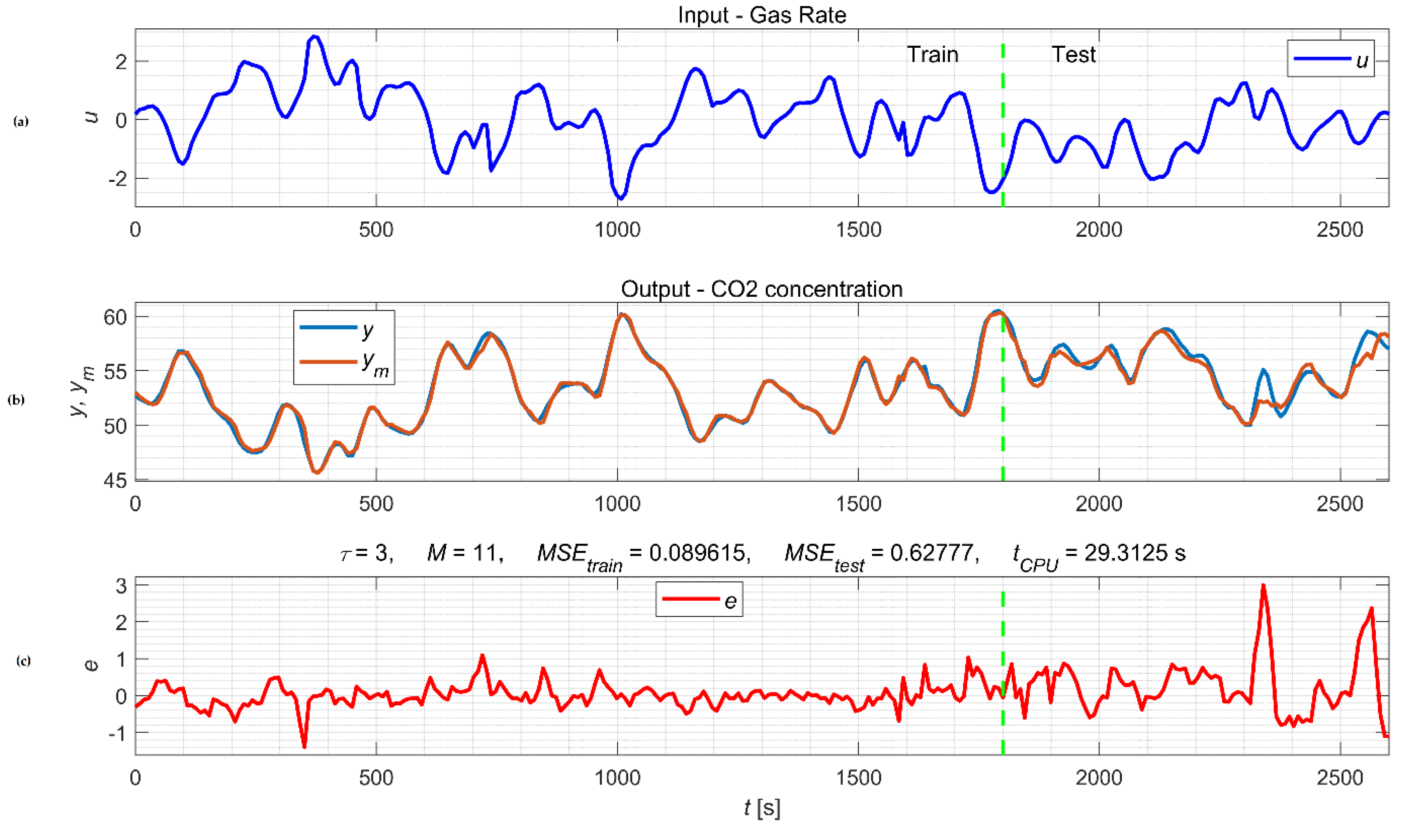
We simulated five cases where we varied the number of M fuzzy sets on each input variable from 5, 7, 11, 13, and 15. Since a WM FS (7) has six input variables, the number of possible rules increases exponentially as the number of fuzzy sets M increases. Accuracy rises with larger M, but at the same time, the processing time tCPU of the training algorithm increases dramatically. The performance result of this fuzzy model is shown in Figure 5, where Figure 5a depicts the original input u of the system, namely gas flow rate, and Figure 5b compares the output of the process y with the predicted output ym of the identified model.
Figure 5b shows the error e between the model output and the predicted process output for the data used for training and for the input test signal. The MSE obtained of our model is 0.08962 by train input signal and 0.62777 by test input signal. By selecting a relatively large number of fuzzy sets M = 11 on the six inputs, we were faced with a large processing time of the training algorithm tCPU = 29.32 s. An important conclusion from testing with WM FS is that, as the number of fuzzy sets M increases, the running time tCPU of the training algorithm increases exponentially. Figure 5b,c shows that the MSEtest of the prediction with the test input signal is much larger than the MSEtrain of the prediction with the training input.
Over the same set of input–output data, all three proposed NARX DCFS structures for output prediction were tested. The results are summarised and presented in Table 2. We first tested out the general NARX DCFS as defined in Definition 1, and with selected parameters, nu = 3, ny = 3, n1 = 4, m 1 = m 2 = 3 ,   m 3 = 2 , and L = 3 are presented in Figure 4a. Such a DCFS structure is characterised by seven FSs with three input variables and one output variable, which are organised into three levels. The inputs are ordered sequentially, as they are written, in the regression vector. For comparison purposes, we have kept the same delay τ but varied the number of fuzzy sets M. As expected, accuracy improved as M increased. Note that the processing time tCPU of the training algorithm increased more slowly with increasing M than in the case of the WM FS, although M is much larger (30 compared to 11). Similarly, we tested the other two proposed NARX DCFS structures, as defined by Definitions 2 and 3 and presented in Figure 4b,c. We observe that the processing time tCPU of the training algorithm is even smaller for the same number of fuzzy sets M. This is the result of fewer inputs to FSs at some levels, and it is a consequence of fewer FSs inputs at some levels, which, in turn, results in a slightly worse MSE performance measure.
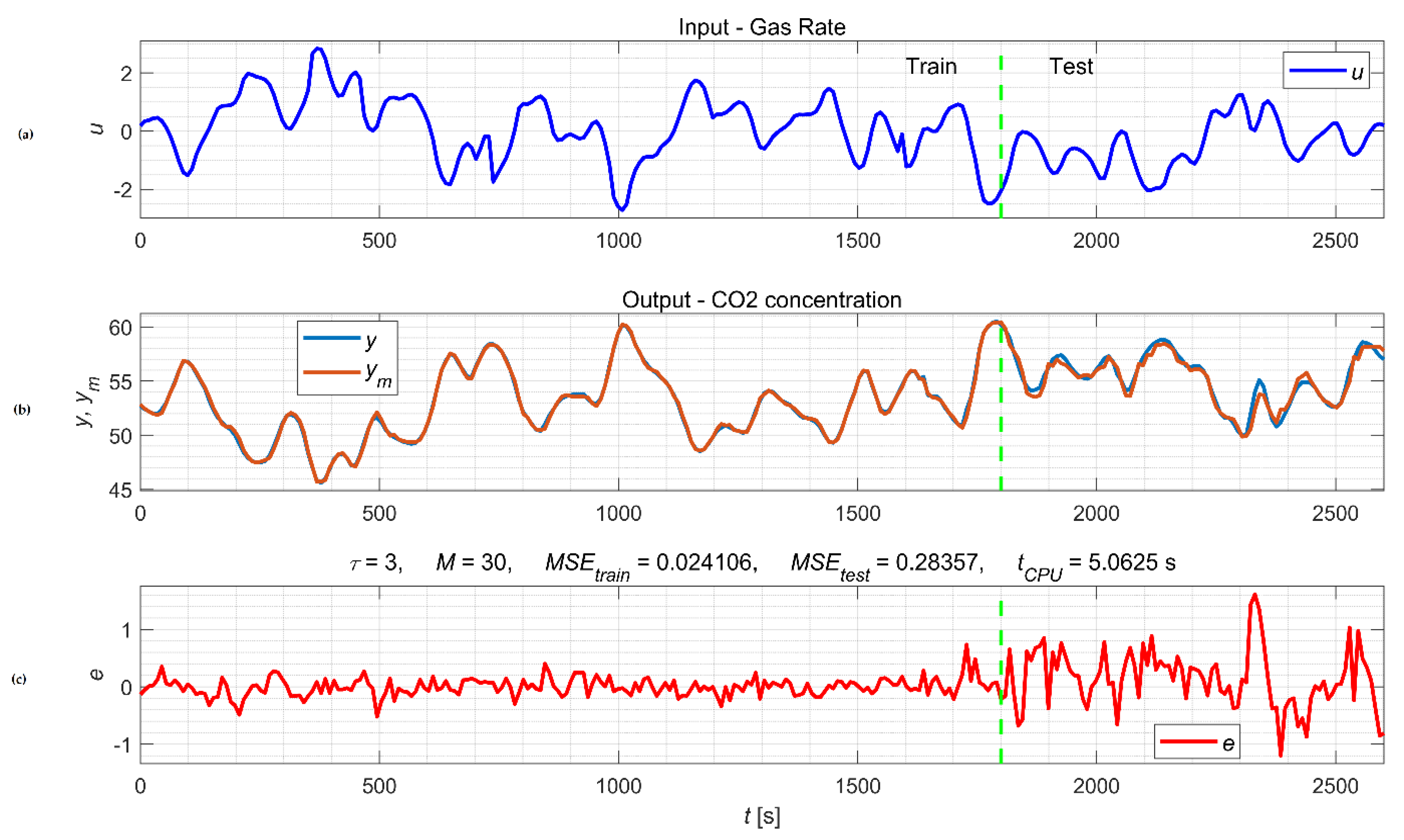
The prediction results are given in Table 2. The results for the General NARX DCFS with M = 30, where we achieved the best performance measures MSEtrain = 0.02411 and MSEtest = 0.28357, are highlighted. The prediction result of General NARX DCFS-based model is shown in Figure 6. The figure indicates that the testing error of the model is larger than the training model. Although we have chosen a relatively large number of fuzzy sets M = 30, the processing time of the training algorithm was relatively small tCPU = 5.07s.
To evaluate the results, we made a comparative analysis of the results of the proposed NARX DCFS structure with other identification methods known from the literature. The methods are different by structure, by the fuzz systems used, and by the methods of learning from the data. We have selected some identification methods [3,4,15,30,31] based on fuzzy relational matrix identification to describe the inference mechanism of the FS. In these methods, we are dealing with comparable learning algorithms, which belong to non-iterative learning methods. We also selected two results based on Sugeno’s fuzzy inference [5,6]. One method is from the field of classical modelling [29]. The three methods described in papers [15,16] are characterised by the use of the FS decomposition principle. The results of these methods compared to NARX DCFS are presented in Table 3.
The table shows that the Sugeno-type FS [5] model is the closest to the General NARX DCFS model in terms of MSE. It should be noted that Sugeno FS is based on rules with linear functions on the consequent side of the rule. Verification result MSE = 0.024 of proposed General NARX DCFS indicates that identification methods based on hierarchical structures, such as the proposed NARX DCFSs, allow for avoiding the use of gradient identification methods and enable the efficient use of identification methods based on a rule extraction approach from data.

3.2. Nonlinear Dynamic Test Processes Identification

The four nonlinear dynamic test systems presented below serve as examples to illustrate the suitability of NARX DCFS for modelling various non-linear processes [2]. They cover different types of non-linear behaviour to demonstrate the universality of the approach.
  • For a Hammerstein system, which is the typical coupling of a static non-linear function and a dynamic linear system, the example is given by a differential equation:
y ( k ) = 0.01867 · a r c t a n [ u ( k 1 ) ] + 0.01746 · a r c t a n [ u ( k 2 ) ] + 1.7826 · y ( k 1 ) 0.8187 · y ( k 2 )
  • As the opposite, a Wiener system is a linear dynamic system in series with a static, non-linear function, and the example is given by a differential equation:
y ( k ) = a r c t a n [ 0.01867 · u ( k 1 ) + 0.01746 · u ( k 2 ) + 1.7826 · t a n ( y ( k 1 ) ) 0.8187 · t a n ( y ( k 2 ) ) ]
  • A nonlinear differential equation (NDE) system is the approximation of a non-minimum phase system of a second order with parameters: gain 1, time constants 4 s and 10 s, and a zero at 0.25 s. Output feedback is a parabolic nonlinearity:
y ( k ) = 0.07289 · [ u ( k 1 ) 0.2 · y 2 ( k 1 ) ] + 0.09394 · [ u ( k 2 ) 0.2 · y 2 ( k 2 ) ] + 1.68364 · y ( k 1 ) 0.70469 · y ( k 2 )
  • A not separable dynamic (NSD) system has a nonlinearity which cannot be divided into a static non-linear part and a dynamic linear part. The behaviour of the system depends on the input variable:
y ( k ) = 0.133 · u ( k 1 ) 0.0667 · u ( k 2 ) + 1.5 · y ( k 1 ) 0.7 · y ( k 2 ) + u ( k ) · [ 0.1 · y ( k 1 ) 0.2 · y ( k 2 ) ]
To identify NARX DCFSs, we excited the non-linear processes with an amplitude modulated pseudo random binary signal (APRBS), which is shown in Figure 7a. APRBS are designed to ensure good excitation of the process at different operating points and are, therefore, suitable for the excitation of non-linear processes. To test the NARX DCFSs, we generated the test signal presented in Figure 7b.
The test signal consists of step functions over the entire range of the input signal, followed by a ramp, and finally ending with a period of the sinusoidal signal.
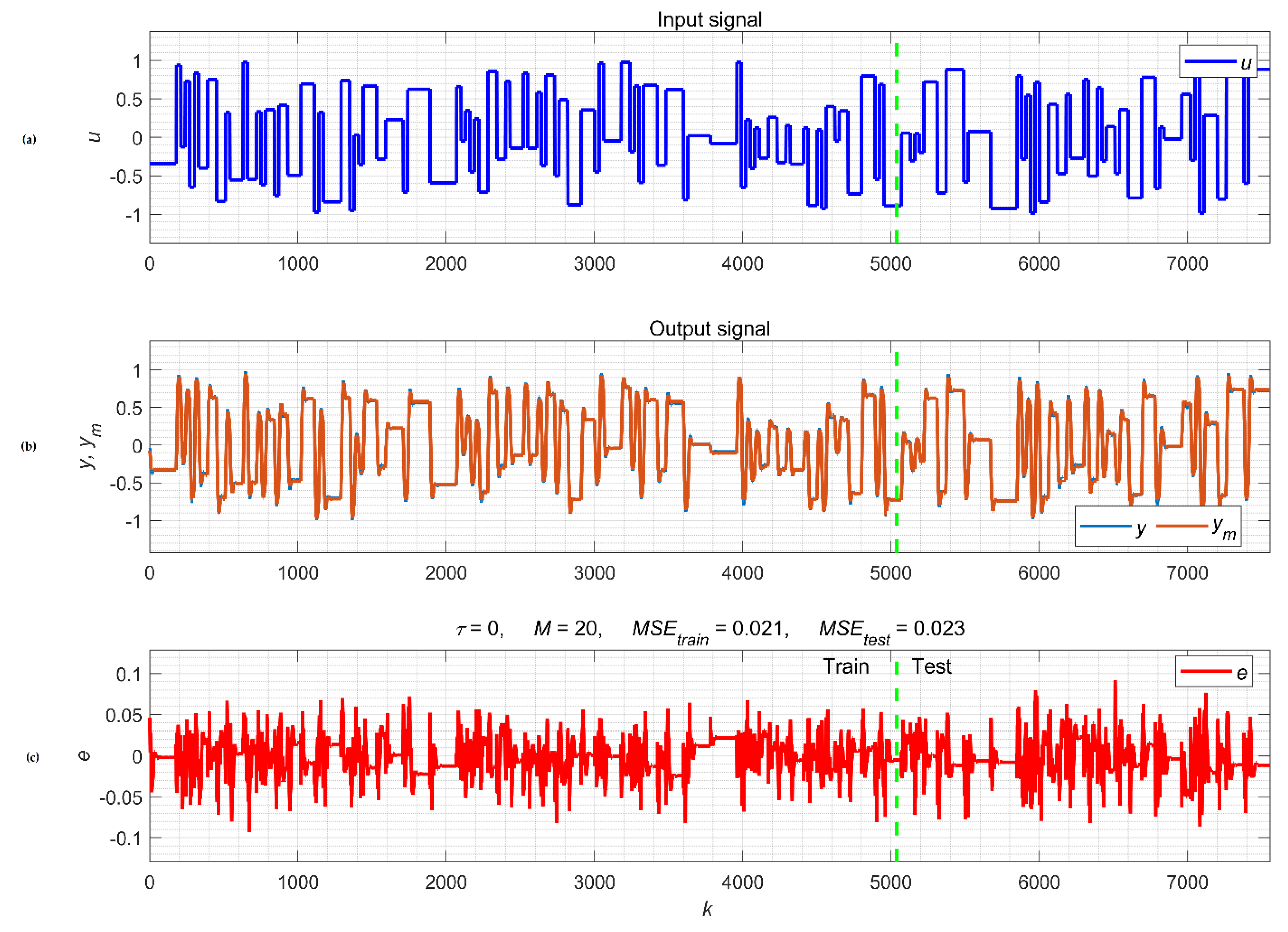
Figure 8 shows the results of training the model with the General NARX DCFS structure to model the first of the four test non-linear processes, namely the Hammerstein system with the parameters given in Equation (17). Figure 8a shows the input signal used for training in a discrete time space from k = 0 to approximately k = 5000, as well as for model testing from k = 5000 to the end. The training and testing results are good, as confirmed by the acceptable MSEtrain = 0.021 and MSEtest = 0.023 values. A comparison of the model output signal y m ( k ) and the output y ( k ) of the process is given in Figure 8b, and the corresponding error e ( k ) is given in Figure 8c. We continued testing with the test signal shown in Figure 9a. Comparison of the results in Figure 9b, where the model output and the process output are presented, shows a good match between the model and the process. The error in the figure is also within acceptable limits. In addition to errors due to transients in step excitation, the largest deviations of the model output from the process output are in the region k = 3400 to k = 3800 and in the k = 6000 to k = 6200.
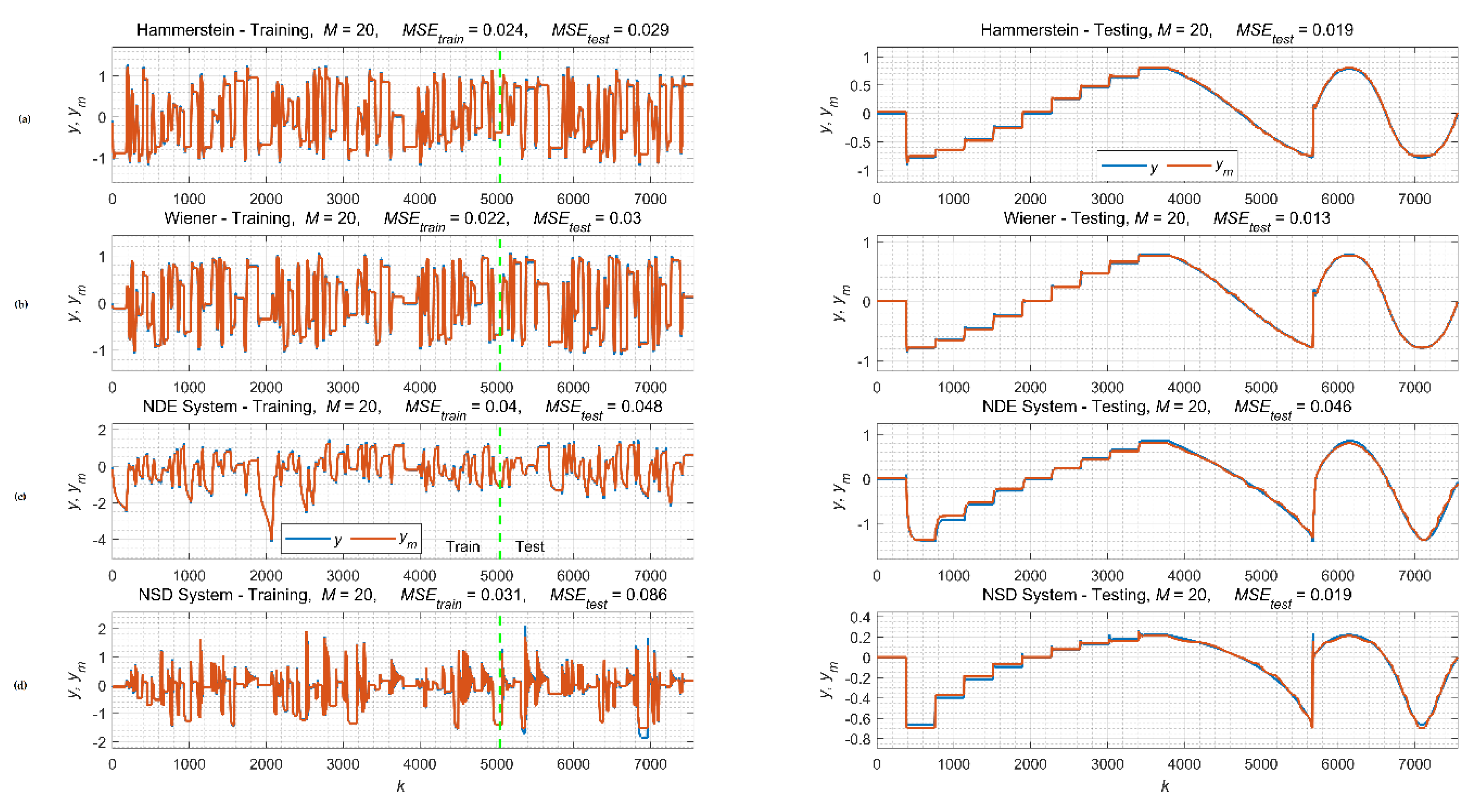
The training and testing results of the other three nonlinear dynamic test processes implemented by Equations (18)–(20) were similar. A slightly worse prediction model was obtained in the case of NDE system identification, which resulted in a larger acceptable MSEtrain and MSEtest. Comparison between all four NDPs and identified NARX DCFS model outputs on training data and test data for all four NDPs is presented in Figure 10.

4. Discussion

We were interested in the modelling results with different combinations of input signals into DCFS and, therefore, we were defined three different families of possible NARX DCFS structures. The first experiment showed, as illustrated by the modelling results presented in Table 2, that all three structures are useful. The results are comparable to the similar WM FS, which, however, requires much more CPU time to execute the training algorithm. Note that, in the case of the presented results we have chosen the simple structures presented in Figure 4, especially in the case of the input–output NARX DCFS structure and the sub-model NARX DCFS structure. Better prediction accuracy is obtained by increasing the number of M fuzzy sets on the input variables of fuzzy systems. In contrast to WM FS, increasing the number of M results in a reasonable increase in the time tCPU required to execute the training algorithm. This is an important advantage of NARX DCFS over WM FS, as M can be scaled up to large numbers, much higher than 30, improving the accuracy of the model prediction.
Figure 8, Figure 9 and Figure 10 show that the results of the second experiment, namely modelling four different types of NDSs for prediction purposes, are also encouraging. The results also show some weaknesses. From the model output responses in Figure 9b and the associated error, an increase in the deviation is seen in the interval from k = 3400 to k = 3800 and, similarly, in the interval from k = 6000 to k = 6200. The error varies depending on the range of the input signal, and in this range, the dynamic system was not sufficiently excited during training. This is due to two reasons. The first is in the input excitation signal, which did not provide enough information in this region to successfully generate FSs’ rules to cover this area. The results can be improved by a more appropriate distribution of the amplitude levels of the excitation input signal presented in Figure 7a. The second reason is an inappropriate choice of the parameter M. If too small of a value is chosen, the training algorithm generates fewer rules, and the result is expressed in worse approximation properties. Comparison of the modelling results of the Hammerstein NDS in Figure 10a and the Wiener NDS in Figure 10b, obtained with the General NARX DCFS structure, shows similar properties. Small deviations are present, which differ from the operating point within the process definition range. Where the process has been adequately excited by the training procedure, the results are better, while others show a slight increase in the deviation between the model and the output of the process. The feature of these two NDSs, a separate non-linear static system and a linear dynamic system, proves to be suitable for modelling with NARX DCFS structures. The order of nonlinearity before the linear system (Hammerstein) or the nonlinearity after the linear system (Wiener) does not significantly affect the result. However, the decoupling of the nonlinear and linear system is not significant for the third and fourth test NDSs. Comparatively, the MSE results are slightly worse, but the deviation is not significant. From Figure 10c,d, we observe slightly more oscillations when tracking the model to the ramp excitation and harmonic signal. Either way, the results are useful for applications with single-step output predictions.
In Table 3, we compare the results of the NARX DCFS modelling with other similar methods. Some are based on fuzzy relational systems with non-iterative training algorithms, and others use FIS, where a combination of linear function rules and training from the data is implemented iteratively. There are several studies that also address neuro-fuzzy modelling of non-linear dynamical systems. We have reviewed recent publications, and the following is a brief overview. In [32], a review of fuzzy and neural prediction interval modelling of nonlinear dynamical systems is presented. The difference between the methods summarised in this review article and our method is that these methods predict a prediction interval, which has the advantage of specifying an interval of model output values. Most of these methods are based on various more-complex FIS structures, such as Type-2 fuzzy system, and use complex iterative training algorithms. Such a FIS was proposed in [33] for predicting the short-term wind power. The advantage of this method over the NARX DCFS is its ability to predict very precisely. The disadvantage lies in the complexity of the learning methods, as it uses the gravitational search algorithm (GSA) for an optimization interval Type-2 fuzzy system. The most similar in concept to our NARX DCFS model is the prediction model proposed in the paper [34] and called the deep neural network-based fuzzy cognitive maps model. It is characterised by both good prediction properties and good possibilities for linguistic interpretation of the results. An alternate function gradient descent, combined with a BP method, is used for a training algorithm. A partial similarity with the NARX DCFS structure can be detected in the study [35], where WM FSs and a combined learning method, consisting of the WM method and a complex-valued neural network, are used to predict dynamic nonlinear systems. The training algorithm is non-iterative. The study [36] presents a similar DCFS with an improved WM method adapted to solve complex classification problems. The use of ANNs to model and predict the outputs of nonlinear systems is a hot research area with many published studies. We highlight this research [37], which presents a new ANN training algorithm based on a hybrid artificial bee colony algorithm that has been used to efficiently approximate nonlinear static systems as well as dynamic systems. Due to the complexity, it is difficult to compare the results with our method. We also reviewed more recent studies [38,39,40,41] that used the same Box and Jenkin’s benchmark in experimental studies. Compared to NARX DCFS, the results are better or comparable. This is a consequence of the proposed more time-consuming training algorithms and optimization methods.
To conclude the discussion, let us summarise the advantages and disadvantages of the proposed method. The good features of the NARX DCFS models are:
  • The hierarchical multilevel structure of DCFS allows the approximator of a non-linear function to be implemented with many more inputs in the regressor vector and without exponential growth in the number of rules.
  • There are many different possibilities when creating a DCFS input vector from a regression vector. This allows us to have different structures. In this work, we present three of them.
  • The training algorithm remains non-iterative, as is typical for DCFS. The N input–output data are processed only once.
  • The ability to predict the output of the nonlinear system is satisfactory.
However, the following drawbacks are also present:
  • The excitation signal must be chosen appropriately, providing both an adequate frequency bandwidth and a large variety of amplitude levels.
  • The results of testing with a training signal are often much better than the results with a test signal, such as in Figure 6b.
  • Once the NARX DCFS parameters and the input signal have been selected, the prediction results cannot be improved by repeating the training procedure.
The above features require further improvements.

5. Conclusions

This study provides a new NARX DCFS model for modelling dynamic nonlinear processes that is simple, allows fast training from input–output data, and does not suffer from the problem of rule explosion in the case when a nonlinear function approximator has many inputs. The main contributions of our study are the definitions of three structures, which differ in the number of hierarchical levels of the DCFS, the number of fuzzy subsystems at each level, the choice of the moving window, and the way in which all fuzzy subsystems are implemented. With the appropriate choice of parameters, practically any FS can be represented as a DCFS. Only minor changes were needed to adapt the DCFS training algorithm to model the NARX DCFS. The experimental results show that NARX DCFS structures are useful for modelling nonlinear dynamical systems where there are many inputs to the static nonlinearity approximator and the speed and convergence of the training algorithm are important, while the accuracy of the model prediction is less relevant.
Our future work will be oriented to research the impact of NARX DCFS system structure on prediction accuracy, as well as applying NARX DCFS models to real process modelling, identification, and control problems.

Supplementary Materials

The following supporting information can be downloaded at: https://www.mdpi.com/article/10.3390/math11020304/s1, S1: MATLAB_Code.zip.

Funding

The author acknowledges the financial support from the Slovenian Research Agency (Research Core Funding No. P2-0028).

Institutional Review Board Statement

Not applicable.

Informed Consent Statement

Not applicable.

Data Availability Statement

Acknowledgments

The author would like to thank the reviewers for their very insightful comments that helped to improve the paper.

Conflicts of Interest

The author declares no conflict of interest.

References

  1. Škrjanc, I.; Iglesias, J.A.; Sanchis, A.; Leite, D.; Lughofer, E.; Gomide, F. Evolving Fuzzy and Neuro-Fuzzy Approaches in Clustering, Regression, Identification, and Classification: A Survey. Inf. Sci. 2019, 490, 344–368. [Google Scholar] [CrossRef]
  2. Nelles, O. Nonlinear System Identification; Springer: Berlin/Heidelberg, Germany, 2001; ISBN 978-3-642-08674-8. [Google Scholar]
  3. Tong, R.M. The Evaluation of Fuzzy Models Derived from Experimental Data. Fuzzy Sets Syst. 1980, 4, 1–12. [Google Scholar] [CrossRef]
  4. Pedrycz, W. An Identification Algorithm in Fuzzy Relational Systems. Fuzzy Sets Syst. 1984, 13, 153–167. [Google Scholar] [CrossRef]
  5. Takagi, T.; Sugeno, M. Fuzzy Identification of Systems and Its Applications to Modeling and Control. IEEE Trans. Syst. Man Cybern. 1985, SMC-15, 116–132. [Google Scholar] [CrossRef]
  6. Sugeno, M.; Yasukawa, T. A Fuzzy-Logic-Based Approach to Qualitative Modeling. IEEE Trans. Fuzzy Syst. 1993, 1, 7. [Google Scholar] [CrossRef] [Green Version]
  7. Su, S.-F.; Yang, F.-Y.P. On the Dynamical Modeling with Neural Fuzzy Networks. IEEE Trans. Neural Netw. 2002, 13, 1548–1553. [Google Scholar] [CrossRef]
  8. Kyoung Kwan Ahn; Ho Pham Huy Anh Inverse Double NARX Fuzzy Modeling for System Identification. IEEEASME Trans. Mechatron. 2010, 15, 136–148. [CrossRef]
  9. Zemouri, R.; Gouriveau, R.; Zerhouni, N. Defining and Applying Prediction Performance Metrics on a Recurrent NARX Time Series Model. Neurocomputing 2010, 73, 2506–2521. [Google Scholar] [CrossRef] [Green Version]
  10. Cogollo, M.R.; González-Parra, G.; Arenas, A.J. Modeling and Forecasting Cases of RSV Using Artificial Neural Networks. Mathematics 2021, 9, 2958. [Google Scholar] [CrossRef]
  11. Ali, W.; Khan, W.U.; Raja, M.A.Z.; He, Y.; Li, Y. Design of Nonlinear Autoregressive Exogenous Model Based Intelligence Computing for Efficient State Estimation of Underwater Passive Target. Entropy 2021, 23, 550. [Google Scholar] [CrossRef]
  12. Rangel, E.; Cadenas, E.; Campos-Amezcua, R.; Tena, J.L. Enhanced Prediction of Solar Radiation Using NARX Models with Corrected Input Vectors. Energies 2020, 13, 2576. [Google Scholar] [CrossRef]
  13. Lewis, F.L.; Campos, J.; Selmic, R. Neuro-Fuzzy Control of Industrial Systems with Actuator Nonlinearities; Frontiers in applied mathematics; Society for Industrial and Applied Mathematics: Philadelphia, PA, USA, 2002; ISBN 978-0-89871-505-7. [Google Scholar]
  14. De Campos Souza, P.V. Fuzzy Neural Networks and Neuro-Fuzzy Networks: A Review the Main Techniques and Applications Used in the Literature. Appl. Soft Comput. 2020, 92, 106275. [Google Scholar] [CrossRef]
  15. Golob, M.; Tovornik, B. Identification of Non-Linear Dynamic Systems with Decomposed Fuzzy Models. In Proceedings of the IEEE International Conference on Systems, Man and Cybernetics, Nashville, TN, USA, 8–11 October 2000; Volume 5. [Google Scholar]
  16. Golob, M.; Tovornik, B. Input-Output Modelling with Decomposed Neuro-Fuzzy ARX Model. Neurocomputing 2008, 71, 875–884. [Google Scholar] [CrossRef]
  17. Raju, G.V.S.; Zhou, J.; Kisner, R.A. Hierarchical Fuzzy Control. Int. J. Control 1991, 54, 1201–1216. [Google Scholar] [CrossRef]
  18. Wang, L.X. A Mathematical Formulation of Hierarchical Systems Using Fuzzy Logic Systems. In Proceedings of the 1994 IEEE 3rd International Fuzzy Systems Conference, Orlando, FL, USA, 26–29 June 1994; IEEE: Orlando, FL, USA, 1994; pp. 183–188. [Google Scholar]
  19. Sun, L.; Huo, W. Adaptive Fuzzy Control of Spacecraft Proximity Operations Using Hierarchical Fuzzy Systems. IEEEASME Trans. Mechatron. 2016, 21, 1629–1640. [Google Scholar] [CrossRef]
  20. Yu, W.; Rodriguez, F.O.; Moreno-Armendariz, M.A. Hierarchical Fuzzy CMAC for Nonlinear Systems Modeling. IEEE Trans. Fuzzy Syst. 2008, 16, 1302–1314. [Google Scholar] [CrossRef]
  21. Kamthan, S.; Singh, H. Hierarchical Fuzzy Logic for Multi-Input Multi-Output Systems. IEEE Access 2020, 8, 206966–206981. [Google Scholar] [CrossRef]
  22. Zeng, X.-J.; Goulermas, J.Y.; Liatsis, P.; Wang, D.; Keane, J.A. Hierarchical Fuzzy Systems for Function Approximation on Discrete Input Spaces With Application. IEEE Trans. Fuzzy Syst. 2008, 16, 1197–1215. [Google Scholar] [CrossRef]
  23. Hinton, G.E.; Osindero, S.; Teh, Y.-W. A Fast Learning Algorithm for Deep Belief Nets. Neural Comput. 2006, 18, 1527–1554. [Google Scholar] [CrossRef]
  24. Wang, L.-X. Fast Training Algorithms for Deep Convolutional Fuzzy Systems with Application to Stock Index Prediction. IEEE Trans. Fuzzy Syst. 2019, 28, 1301–1314. [Google Scholar] [CrossRef]
  25. Wang, L.-X.; Mendel, J.M. Generating Fuzzy Rules by Learning from Examples. IEEE Trans. Syst. Man Cybern. 1992, 22, 1414–1427. [Google Scholar] [CrossRef] [Green Version]
  26. Wang, L.-X. The WM Method Completed: A Flexible Fuzzy System Approach to Data Mining. IEEE Trans. Fuzzy Syst. 2003, 11, 768–782. [Google Scholar] [CrossRef]
  27. Jang, J.-S.R. ANFIS: Adaptive-Network-Based Fuzzy Inference System. IEEE Trans. Syst. Man Cybern. 1993, 23, 665–685. [Google Scholar] [CrossRef]
  28. Golob, M.; Tovornik, B. Decomposed Neuro-Fuzzy ARX Model. In Advances in Soft Computing—AFSS 2002; Pal, N.R., Sugeno, M., Eds.; Lecture Notes in Computer Science; Springer: Berlin, Heidelberg, 2002; Volume 2275, pp. 260–266. ISBN 978-3-540-43150-3. [Google Scholar]
  29. Box, G.E.P.; Jenkins, G.M. Time Series Analysis: Forecasting and Control; Holden-Day: San Francisco, CA, USA, 1970; ISBN 978-0-8162-1094-7. [Google Scholar]
  30. Xu, C.; Lu, Y. Fuzzy Model Identification and Self-Learning for Dynamic Systems. IEEE Trans. Syst. Man Cybern. 1987, 17, 683–689. [Google Scholar] [CrossRef]
  31. Branco, P.J.C.; Dente, J.A. A New Algorithm for On-Line Relational Identification of Nonlinear Dynamic Systems. In Proceedings of the 1993 Second IEEE International Conference on Fuzzy Systems, San Francisco, CA, USA, 28 March–1 April 1993; IEEE: San Francisco, CA, USA, 1993; pp. 1173–1178. [Google Scholar]
  32. Cartagena, O.; Parra, S.; Munoz-Carpintero, D.; Marin, L.G.; Saez, D. Review on Fuzzy and Neural Prediction Interval Modelling for Nonlinear Dynamical Systems. IEEE Access 2021, 9, 23357–23384. [Google Scholar] [CrossRef]
  33. Zou, W.; Li, C.; Chen, P. An Inter Type-2 FCR Algorithm Based T–S Fuzzy Model for Short-Term Wind Power Interval Prediction. IEEE Trans. Ind. Inform. 2019, 15, 4934–4943. [Google Scholar] [CrossRef]
  34. Wang, J.; Peng, Z.; Wang, X.; Li, C.; Wu, J. Deep Fuzzy Cognitive Maps for Interpretable Multivariate Time Series Prediction. IEEE Trans. Fuzzy Syst. 2021, 29, 2647–2660. [Google Scholar] [CrossRef]
  35. Xue, C.; Mahfouf, M. A New Deep Complex-Valued Single-Iteration Fuzzy System for Predictive Modelling. In Proceedings of the 2022 IEEE International Conference on Fuzzy Systems (FUZZ-IEEE), Padua, Italy, 18–23 July 2022; IEEE: Padua, Italy, 2022; pp. 1–7. [Google Scholar]
  36. Wang, Y.; Liu, H.; Jia, W.; Guan, S.; Liu, X.; Duan, X. Deep Fuzzy Rule-Based Classification System With Improved Wang–Mendel Method. IEEE Trans. Fuzzy Syst. 2022, 30, 2957–2970. [Google Scholar] [CrossRef]
  37. Kaya, E. A New Neural Network Training Algorithm Based on Artificial Bee Colony Algorithm for Nonlinear System Identification. Mathematics 2022, 10, 3487. [Google Scholar] [CrossRef]
  38. Yan, S.; Zhou, J.; Zheng, Y.; Li, C. An Improved Hybrid Backtracking Search Algorithm Based T–S Fuzzy Model and Its Implementation to Hydroelectric Generating Units. Neurocomputing 2018, 275, 2066–2079. [Google Scholar] [CrossRef]
  39. Ustundag, B.B.; Kulaglic, A. High-Performance Time Series Prediction With Predictive Error Compensated Wavelet Neural Networks. IEEE Access 2020, 8, 210532–210541. [Google Scholar] [CrossRef]
  40. Waheeb, W.; Ghazali, R. Forecasting the Behavior of Gas Furnace Multivariate Time Series Using Ridge Polynomial Based Neural Network Models. Int. J. Interact. Multimed. Artif. Intell. 2019, 5, 126. [Google Scholar] [CrossRef] [Green Version]
  41. Lyu, J.; Liu, F.; Ren, Y. Fuzzy Identification of Nonlinear Dynamic System Based on Selection of Important Input Variables. J. Syst. Eng. Electron. 2022, 33, 737–747. [Google Scholar] [CrossRef]
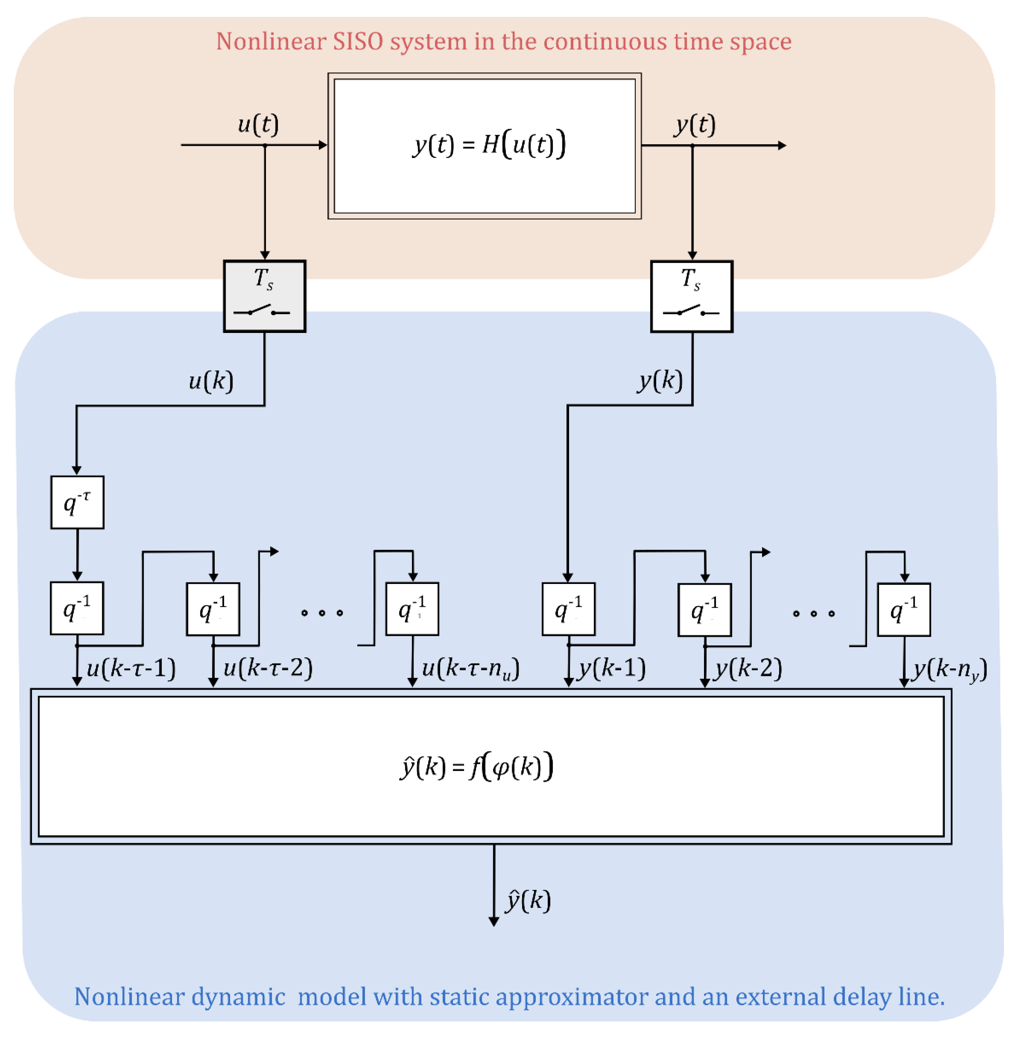
Figure 1. Nonlinear dynamic system modelling structure based on external dynamics strategy.
Mathematics 11 00304 g001
Figure 2. Membership functions of the FS with m inputs x and one output y.
Mathematics 11 00304 g002
Figure 3. General structure of a DCFS with moving window size m l = 3 .
Mathematics 11 00304 g003
Figure 4. Different NARX DCFS structures are possible, and three are presented: (a) general structure of a NARX DCFS, (b) input–output NARX DCFS structure, and (c) sub-model NARX DCFS structure.
Mathematics 11 00304 g004
Figure 5. Comparison of WM FS model output and original system output for Box and Jenkin’s gas furnace data set: (a) input signal—gas rate, (b) outputs comparison, and (c) respective error. The green line divides the training data from the test data.
Mathematics 11 00304 g005
Figure 6. Prediction result of General NARX DCFS model output and original system output for Box and Jenkin’s gas furnace data set: (a) input signal—gas rate, (b) output comparison, and (c) respective error. The green line divides the training data from the test data.
Mathematics 11 00304 g006
Figure 7. Input signals for the nonlinear processes identification with NARX DCFS: (a) excitation input signal is an amplitude modulated pseudo random binary signal; (b) testing input signal.
Mathematics 11 00304 g007
Figure 8. Comparison between desired outputs y and predicted outputs ym for the Hammerstein nonlinear dynamic test process obtained in the training session: (a) amplitude modulated pseudo random binary signal (APRBS); (b) model output signal y m and the output y of the process; (c) model error e . A dotted green line separates the training area and the testing area.
Mathematics 11 00304 g008
Figure 9. Comparison between desired outputs y and predicted outputs ym for the Hammerstein nonlinear dynamic test process obtained in the testing session: (a) testing input signal; (b) model output signal y m and the output y of the process; (c) model error e .
Mathematics 11 00304 g009
Figure 10. Comparison between desired outputs y and predicted outputs ym for the nonlinear dynamic test processes: (a) Hammerstein, (b) Wiener, (c) NDE, and (d) NSD. The left-hand side shows the training data session results, and the right-hand side the test data session results.
Mathematics 11 00304 g010
Table 1. Structures of regression vectors for common input/output models.
ModelRegression Vector φ(k)
NTS φ ( k ) = [ y ( k 1 ) , y ( k n y ) ]
NARX φ ( k ) = [ y ( k 1 ) , y ( k n y ) , u ( k 1 ) , u ( k n u ) ]
NARMAX φ ( k ) = [ y ( k 1 ) , y ( k n y ) , u ( k 1 ) , u ( k n u ) , e ( k 1 ) , e ( k n y ) ]
OE φ ( k ) = [ y ^ ( k 1 ) , y ^ ( k n y ) , u ( k 1 ) , u ( k n u ) ]
Table 2. Comparison of the performance of the proposed methods in Box–Jenkins system identification problem.
Model τ MMSEtrainMSEtesttCPU [s]
350.282350.760691.10
370.178430.542433.21
WM FS (7) [26]3110.089620.6277729.32
3130.056810.5512094.25
3150.040510.90677261.52
350.493030.381330.79
General NARX DCFS3150.110420.324131.83
3300.024110.283575.07
350.455350.500220.77
Input-output NARX DCFS3150.122080.246391.18
3300.045370.44843.58
350.382980.596550.50
Sub-model NARX DCFS3150.130690.349040.85
3300.036970.582401.11
Table 3. Identification results for the Box–Jenkins gas furnace.
ReferenceNo. of VariablesMSE
Box Jenkins [29]-0.71
Tong [3]y(k-1), u(k-4)0.469
Pedrycz [4]y(k-1), u(k-4)0.320
Xu [30]y(k-1), u(k-4)0.328
Costa Branco [31]y(k-1), u(k-4)0.312
Sugeno-Yasukawa [6]y(k-1), y(k-2), y(k-3)
u(k-1), u(k-2), u(k-3)
0.190
Takagi Sugeno [5]y(k-1), u(k-3), u(k-4)0.068
Golob ARX min-max [15]y(k-1), u(k-4)0.73
Golob ARX sum-prod [15]y(k-1), u(k-4)0.57
Golob DNF ARX [16]y(k-1), u(k-4)0.196
General NARX DCFSy(k-1), y(k-2), y(k-3),
u(k-4), u(k-5), u(k-6)
0.024
Disclaimer/Publisher’s Note: The statements, opinions and data contained in all publications are solely those of the individual author(s) and contributor(s) and not of MDPI and/or the editor(s). MDPI and/or the editor(s) disclaim responsibility for any injury to people or property resulting from any ideas, methods, instructions or products referred to in the content.