Article

Study on the Stiffness and Dynamic Characteristics of a Bridge Approach Zone: Tests and Numerical Analyses

1
Department of Engineering Management, Hunan University of Finance and Economics, Changsha 410205, China
2
School of Civil Engineering, Central South University, Changsha 410018, China
*
Author to whom correspondence should be addressed.
Mathematics 2023, 11(19), 4202; https://doi.org/10.3390/math11194202
Submission received: 6 September 2023 / Revised: 1 October 2023 / Accepted: 4 October 2023 / Published: 8 October 2023

Abstract

:
This study focuses on the stiffness and dynamic characteristic rules of a bridge approach zone in a high-speed railway (HSR). Indoor and in situ tests were performed to explore the stiffness and dynamic characteristics of the roadbed filling. Based on the test results, an effective track-subgrade finite element model (FEM) of a high-speed train (HST) was established. The FEM simulated the train load and model boundaries based on the obtained loads and viscoelastic artificial boundaries. Suitable elements were then selected to simulate the various components of the system and the constraint equations were established and solved using multi-point constraints. The model was verified by comparing the time–history curve characteristics, the frequency-domain characteristics and the results obtained from different modeling methods with the measured results. The influence of stiffness on the dynamic characteristics of the bridge approach zone were subsequently analyzed based on the aforementioned tests and simulations. The results indicate that (i) the model produced reliable results using the proposed approach; (ii) the influence of train load on the embankment was generally reflected in the upper part of the structure, and thus, bed structures are recommended to be strengthened; and (iii) under stationarity, the stiffness ratio between the bridge and normal subgrade is recommended as 1:6, with a transition length of 25 m.

1. Introduction

Transition zones are special structures that connect numerous components in high-speed railways (HSRs) such as bridges, culverts and tunnels. The strength, deformations and stiffness of which are distinct from normal subgrade, which inevitably results in settlement differences, and thus represent the weakest sections under high-speed train loads [1,2,3,4]. Cristina [5] conducted on-site tests on the transition zone of a culvert at a Portuguese HSR, revealing that the track displacement of the structure and reinforcement zone were 45% and 30% lower than that of the roadbed, respectively, with minimal changes in longitudinal acceleration along the line. European scholars have suggested that more research needs to focus on transitions [6,7,8]. Researchers in the USA [9,10,11] determined that the stiffness ratio between the bridge and normal subgrade can reach up to 2. Compared with normal tracks, the transition section requires four times more maintenance and double the costs. Therefore, research into the stiffness and dynamic properties of transition zones is critical for the stability of HSRs.
Numerous studies have investigated the dynamic characteristics of transition zones using field tests and by analyzing the dynamic responses of the track and subgrade [5,12,13,14], most of which focus on standard railway lines with low train speeds. Additional research has examined the stiffness variation law by wave tests, excitation experiments and analyzing the elastic modulus and dynamic stiffness along the transition [15,16,17]. However, the majority of these studies test the index solely on the test point rather than targeting the index in the entire cross-section. Bonopera [18], Wang [19] investigated the stiffness and dynamic characteristics of concrete bridges using experimental tests on simply supported prestressed concrete beam specimens.
The aforementioned research has made great progress in furthering our understanding and providing reference for the dynamic and stiffness characteristics of transition zones. However, such studies are difficult to carry out as they require special organization, as well as extensive manpower and financial resources. Therefore, simulation analysis has become a supplement to investigate the dynamic characteristics of the transition zones of high-speed railways.
Heydari [20] established a three-dimensional train-track model to evaluate the dynamic characteristics of the transition section connecting ballasted and ballastless tracks, without considering the vibration of the roadbed for simplification. Fu [21,22] modeled and analyzed the transition section based on wave analysis, and suggested that gradual changes in the stiffness of the transition section can enhance the dynamic stability of the track roadbed. Chen [23] proposed a new method based on Green’s function to effectively simulate the vertical dynamic interaction of vehicle track subgrade. The system is divided into two subsystems, namely, the vehicle track subsystem and the slab subgrade subsystem, which are coupled through fastener connections. However, the establishment of the track-subgrade system induced by trains in transition zones requires further investigation in terms of several key properties. These include determining how to simulate both the train load and subgrade, how to correctly and effectively simulate the energy radiation of infinite foundation, how to simulate the damping of the CA (cement asphalt) mortar layer and how to eliminate and handle different units of freedom of rotation.
Therefore, based on the objective of studying the dynamic and stiffness characteristics of transition zones from experimental tests and numerical simulations, this paper initially investigated the basic properties of roadbed filling and stiffness characteristics in transition zones using experiments. We then established an effective three-dimensional train-track-subgrade model by (i) determining the wheel-rail force in the transition and normal sections by rail acceleration; (ii) reducing the model size through manual boundary processing; (iii) establishing and solving the constraints of different elements of the model; and (iv) verifying the model under different perspectives. Following this, we calculated and analyzed the comprehensive stiffness and dynamic characteristics of a bridge approach via experiments and numerical simulations.

2. Experiments

The testing section selected for the experiments was a bridge approach with a 3.5 m height filling roadbed located in the Wuhan Guangzhou HSR. The tail section of the bridge contains section DK1252 + 887.27, followed by a regular trapezoid approach in DK1252 + 885, which gradually heads towards the normal embankment. The foundation is reinforced by 0.5 m-diameter CFG piles. The bed surface is made up of 0.4 m thick graded crushed stones, and the bottom layer of the roadbed is filled with group A and B fillers.

2.1. Trial Run Test

Figure 1 presents the longitudinal section of the bridge approach. In bridge tail section DK1252 + 855, the vibration sensors were buried on the surface and bottom of the bed surface, the center and the bottom of the subgrade to test the dynamic responses of each layer and to verify the model (Section 4). Two accelerometers were attached to the waist of the rail in transition section DK1252 + 885 (bridge tail) and embankment section DK1252 + 863 (normal subgrade) to test the rail acceleration and determinate the train load (Section 3.2). The data were collected with an imc CL-5016-ET data-acquisition system (Germany) at the sampling frequency of 1000 Hz, and processed using the imc famos 7.4-software (Berlin, Germany).
Two operating vehicles were used for the trail run tests. The first was a CHR2-type HST, consisting of six motor trains and two trailers, with a 14-ton train axle, a 2.5 m long fixed wheelbase bogie, and a 4.2 m long front and rear wheelbases. The operating speed gradually increased from 200 km/h to 350 km/h. The second vehicle was a track inspection train with a 25-ton axle load and operating speed of 160 km/h.
During the construction process, 891-2 type velocity sensors with a 1 × 10⁻⁶ m accuracy were buried on the top of the bed surface. In addition, DYB-5 type resistance strain dynamic earth pressure boxes with a 0.05–1.0 MPa range, 0.083% F•S resolution and 0.8% F•S integrated error were buried on the top of the bed bottom layer. After testing the dynamic responses, the physical units were calibrated and the trend items were removed to preprocess the dynamic response test data.
Trail tests were performed during the joint debugging and testing period in the early stage of construction. The test data were collected using the imc CL-5016-ET acquisition instrument with a sampling frequency of 1024 Hz. The instrument was calibrated and interconnected by shielded cables. The analysis software was calibrated before testing.
Figure 2 depicts the typical time–history curves of dynamic acceleration following preprocessing. The loading and unloading processes of the wheelset and the train carriages are clearly distinguishable in the time–domain curves. The close distance between the rear bogies of the front carriage and the front bogies of the rear carriage creates a superimposed effect on the dynamic load of the wheel sets. Therefore, the peak response of each adjacent bogie during the action process is taken as the sample data. Thus, N-1 sample data can be extracted from each driving record, where N is the number of carriages. After removing significant abnormal data, the upper limit of the 95% confidence interval was calculated as the dynamic response amplitude for the subsequent analysis.

2.2. Indoor Parameter Experiments

The bed fillings of the bridge approach include group A and B fillers, graded crushed stone and graded crushed stone with 5% cement, each with a maximum particle size close to 60 cm (coarse particle fillers). In order to maximize the accuracy of the modeling parameters, particle size analysis, compaction testing and triaxial compression testing of the bed fillings were performed according to the Code for Soil Tests of Railway Engineering [24].
The uniformity coefficient of the graded crushed stone and group A and B fillers were determined as 16.2 and 26, respectively, both of which are greater than 10. Moreover, the curvature coefficient of the graded crushed stone and group A and B fillers were calculated as 1.44 and 2.67, respectively, lying within the interval [1,3]. Thus, the two grading indicators meet the requirements for railway subgrade filling materials.

2.3. In Situ Wave Velocity Testing

The dynamic modulus, dynamic Poisson’s ratio and other dynamic parameters are key indices for the dynamic analysis model. Thus cross-hole and down-hole wave velocity tests were conducted in sections +855 (normal subgrade), +880 (bridge approach) and +887 (bridge tail) according to the Code for the Measurement Methods of the Dynamic Properties of Subsoils [25].
Figure 3 depicts the schematic diagram of the drilling arrangement for the wave test. The experiment adopted a linear arrangement of drilling holes with one hole for excitation and two holes for reception. The holes had an aperture of 127 mm and depths of 6 m and 9 m according to the roadbed height at different measurement points. The gaps around the casing were filled with cement mortar. Table 1 reports the test results.
Table 1 reveals that the aforementioned dynamic parameters vary considerably. This is attributed the type of filling material rather than the roadbed depth. Comparing the dynamic parameters of different materials shows that the wave velocity propagates fastest in graded crushed stone + 5% cement, followed by graded crushed stone, with group A and B fillers exhibiting the slowest propagation. This agrees with the results of Ed and Gd. However, Poisson’s ratio is the opposite, which is consistent with the inverse ratio of the elastic modulus to Poisson’s ratio.
Moreover, the test results of the down-hole method are slightly lower than those of the cross-hole method. This is due to the synergistic relationship between the structural plane features and the direction of the test section during cross-hole testing.

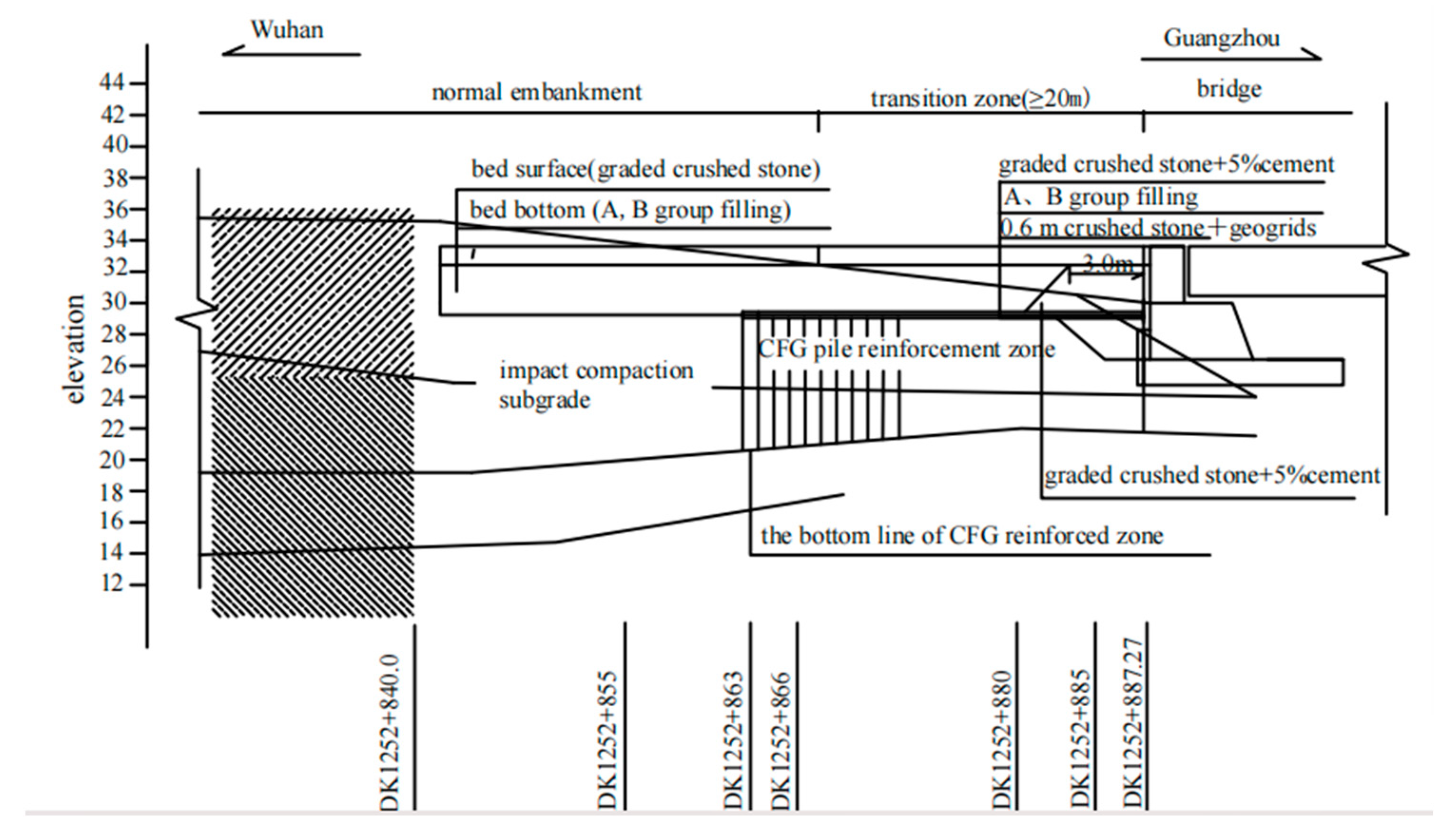
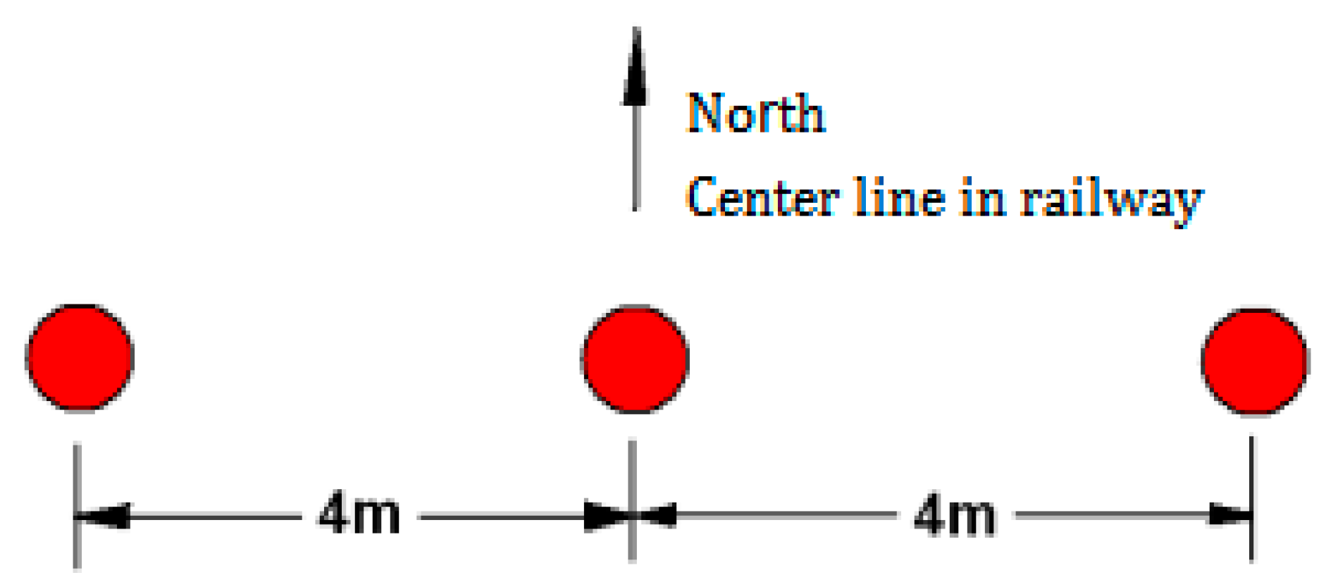
2.4. In-Situ Excitation Experiment

We performed an excitation experiment to obtain the dynamic rigid parameters and verify the simulation results. Figure 4 presents the methodological principle used for the excitation tests, which were carried out in sections +853, +880, +866 and +887.
Two C30-concrete model blocks were prefabricated, with hanging rings preset at the four corners. Four 20 mm diameter and 400 mm long bolts were embedded in the center of the block to fix the excitation motor, ensuring that the disturbance line of the excitation machine passes through the center of gravity and the center of the bottom surface during operation. An intelligent frequency converter was used to adjust the vertical vibration frequency of the excitation motor. Different frequencies were adopted to force the transition section structural layer to vibrate, with 941-type sensors used to pick up the vibration signals. The signals were amplified and converted into digital signals via a signal amplifier and INV306 dynamic signal acquisition instrument. The vibration frequency and amplitude of the system under this frequency of forced vibration were recorded. The excitation frequency ranged from 5 Hz to 50 Hz, and the test data were measured at every 1 Hz increment.
The curves of vertical amplitude variation with frequency are shown in Figure 5. And the results are shown in Table 2.

3. Numerical Modelling

3.1. Dynamics Fundamentals

The model was implement using ANSYS (ANSYS, Inc., Canonsburg, PA, USA) [26]. In the model, the bridge was established at 6 m, and the total bridge approach length was 58.2 m. Figure 6 presents the single-line model, which accounts for the symmetry of the two-line structure of the HSR. The model specifications are described in the following.
Parameters: Table 3 lists the model parameters. The asterisks denote the parameters determined by the tests, while the remaining parameters were obtained from references.
Damping: We adopted Rayleigh damping for the model.
Constitutive model: A viscoelastic constitutive model was used here with a spring and glue pot parallel connection, where and were obtained via wave and excitation tests, respectively.
Boundary constraint: For the bridge, a fixed constraint was applied for its great stiffness.
For the bridge approach and normal embankment, a viscoelastic artificial boundary was adopted (Figure 6b). Figure 7 presents the specific implementation method, where X and Y are the tangential directions along the artificial boundary, and Z is the normal direction. The physical component parameters of the viscoelastic artificial boundary nodes are described as
K 1 = K 2 = 2 G R i = 1 I A i ,   C 1 = C 2 = ρ c s i = 1 I A i ,   K 3 = 4 G R i = 1 I A i ,   C 3 = ρ c p i = 1 I A i  
where A i is the area represented by the nodes on the artificial boundary, with I = 4 in Figure 5; R denotes the radial coordinates, ρ is the density of medium, and G, cs, cp were determined via wave speed tests (Table 3).

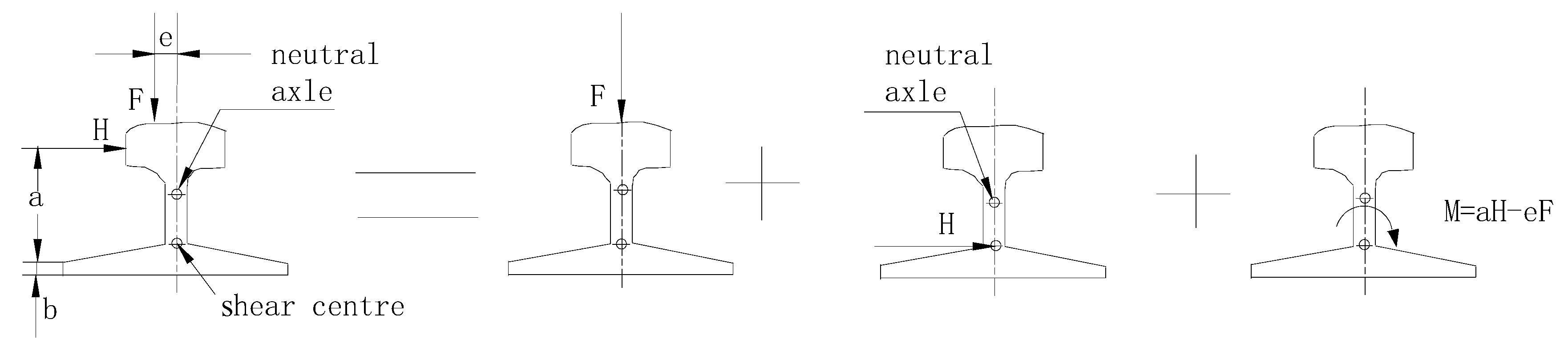
3.2. Modeling of Train Load

Train load is always simplified by a moving wheel rail force. What is different in this paper is that the vibration caused by the train was regarded as a stationary Gaussian process [27,28]. The wheel rail force were determined via test rail acceleration.
Determination of train load: The train load was simulated via the following steps: (i) rail acceleration time–history curve was obtained via testing, (ii) the wheel–rail force time–history curve was determined from the test data, (iii) the wheel–rail forces in the bridge approach and normal embankment were obtained and subsequently applied in the model.
Measured acceleration and deterministic load: In the discrete sampling of vertical orbit vibration acceleration waveform, N was assumed to equal 1024, and the measured acceleration time–history curve after filtering at 330 km/h is shown in Figure 8a,b, whereas the determined wheel–rail interaction force time–history curves are depicted in Figure 8c,d.
The results indicate that the wheel–rail force of section DK1252 + 885 fluctuates by around 30 kN with a maximum amplitude of 63 kN and a minimum of 7 kN, while the wheel–rail force of section DK1252 + 863 fluctuates by around 27 kN with a maximum amplitude of 57 kN and a minimum of 6 kN.
Comparison of vibration loads: The determined wheel–rail force was compared with the measured wheel–rail force of a Rheda2000 type ballastless track provided by ASTRI [24,29,30], and the obtained results are shown in Table 4. There was only a difference of 3.8% in the transition section and a difference of 9.9% at the ordinary embankment between the determined and measured results. The test location of the ASTRI was in a curved embankment, while the location of the accelerometer used in this paper was in a straight line. This difference inevitably leads to a difference in wheel–rail force.
Train load modelling: As shown in Figure 9, let the longitudinal length of the train be l and let the train speed be v. At the beginning, the train is located on node 1, while the train dynamic load p1(t) acts on node 1, then the load p2(t) acts on node 2 after l/v seconds when the train reaches Section 2, and so on. It was assumed that the train passed Section 1 completely after t0 s and the train load ceased to act on node 1, then the train passed Section 2 completely after t0 + l/v s, and the train load ceased to act on node 2, and so on.
For the bridge approach zone, the wheel-track force time–history curve of each node on the rail is different for a bridge, an embankment and the transition. However, due to the limited number of buried components, some simplifications and assumptions must be made in the train–load simulation. In the actual calculation, the load of the transition section is simulated by the data of the DK1252 + 885 section, while the load of common subgrade is simulated by the data of section DK1252 + 863.

3.3. Track and Subgrade

The elements and dimensions of the model are illustrated in Table 5. The mesh size is 0.6–1 m. The structures of HSR are as follows:
The rail is the first layer. It was made of No.60 rail in Japan and the cross section was an “I”-shaped beam; the space between rails is 1435 mm. Beam element BEAM188 is good for simulating the rail.
The second layer is the fasteners and sub-track rubber cushion system with initial length of 38 m, which was simulated by a spring and damping element COMBIN14.
The third layer is the track plate. Due to the extremely thin thickness (190 mm) of the track board compared to its length (4930 mm) and width (2340 mm), with ratios of about 1/26 and 1/12, respectively, the track board layer is simulated by shell element SHELL143 instead of a solid element.
The fourth layer is cement asphalt (CA) mortar. It is an important link in improving the elasticity of slab track and mitigating vibration. On the one hand, considering the flexural deformation of CA mortar under train load, and on the other hand, considering the vibration reduction effect of the CA mortar layer. It is simulated by shell element SHELL143 and a spring damping element instead of shell element SHELL143.
The fifth to eighth layers were C20 concreate supporting layer, roadbed and subgrade. Solid element SOLID45 is suitable to simulate it.

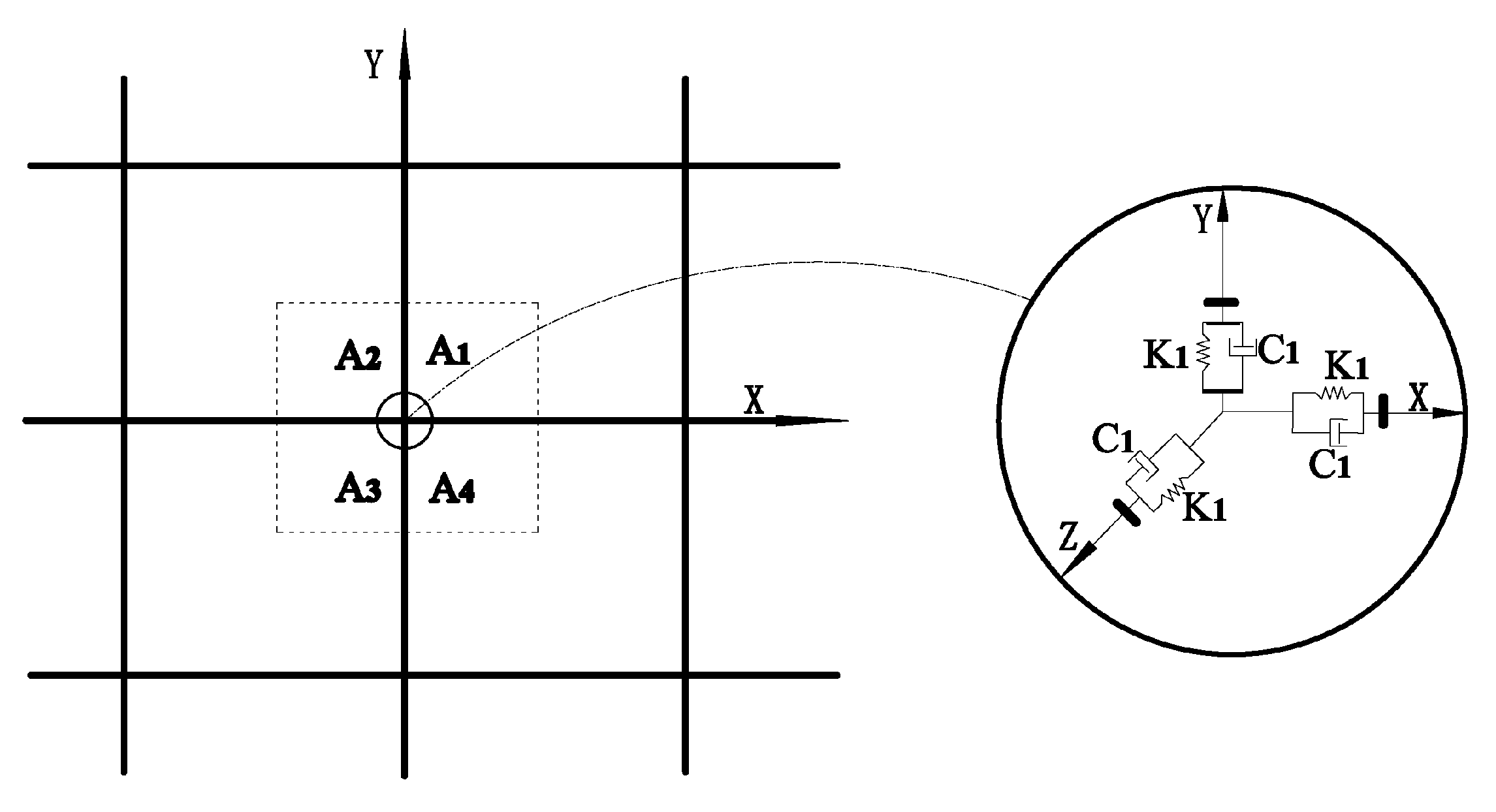
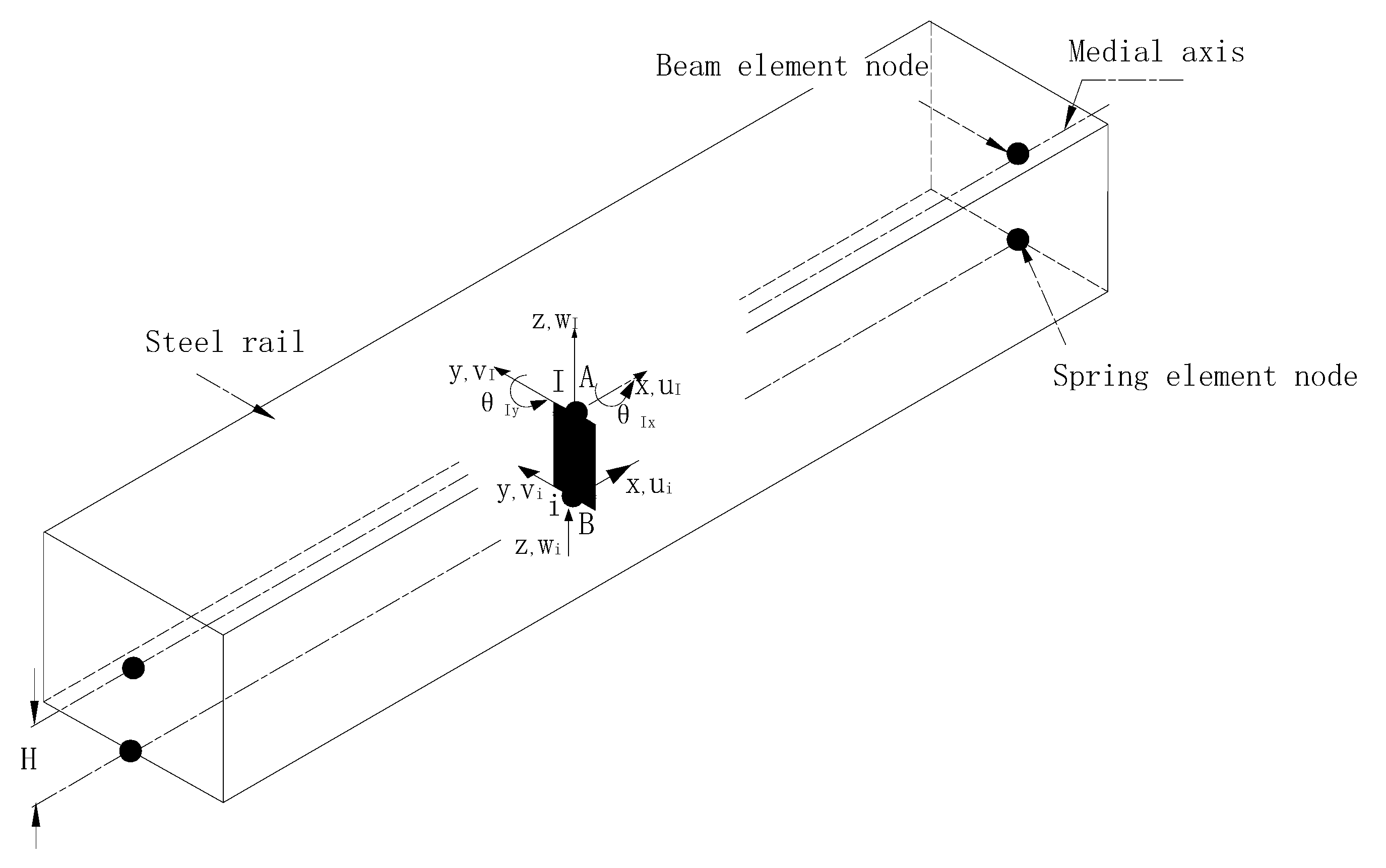
3.4. Establishment of Multi-Point Constraint Equations

In this study, direct introduction method was used to obtain the constraint equations of different type elements, then the equations were introduced into the weak integral form of Galerkin method and transferred to solid stiffness matrix and load vectors. Finally, equation solutions were obtained by forming the system stiffness matrix and load vectors from gathering the shell or beam stiffness matrix or load vector. The last step was to calculate the numerical solution of the equations.
The offset connections include that between beam axis and spring element, that between spring element and shell element, that between shell–shell elements and that between shell–solid element connection. However, for lack of space, only the first two linking methods will be explained as follows.
(1)
Offset connection between beam axis and spring element
While the vehicle is running on the track, the vertical wheel loads are not forced in the centerline of the track and the transverse loads are not exerted in shear-three-center of the track section, which causes torsion movement on the track. Under general conditions, the track’s vertical and transverse displacements and rotation angles are independent from each other, all of which could be superposed linearly and thus the three aspects may be considered, respectively, as shown in Figure 10. As for the sub-track dynamic response, only the action of vertical wheel loads was considered.
As seen in Figure 11, in terms of mechanism conditions, it could be assumed that the track, fasteners and sub-track rubber cushion under the unballasted track of HSR are hinged and the track is able to rotate freely and with the same displacements at interfaces.
If the fasteners and sub-track rubber cushion are stimulated by spring elements and the track by a beam element is able to rotate freely, both the longitudinal symmetric globe z-axis through the spring element’s node i and middle surface’s normal through the beam element’s node I are at the same line. Moreover, It in the beam element’s normal and ib in the longitudinal symmetric axis of the spring element are connected; after deformation, the line remains linear and unchanged, viz., the line I-It-ib-i still remains linear, and It and ib remain connected. Thus, the multi-point constraint equations are as following, when the beam element is below the spring elements:
u i = u I H θ y I       or       u i u I + H θ y I = 0
v i = v I + H θ x I         or         v i v I H θ x I = 0
w i = w I ,       or           w i w I = 0
Equations (2)–(4) was then written using matrix forms:
[ u i v i w i ] = [ 1 0 0 0 H 0 1 0 H 0 0 0 1 0 0 ] [ u I v I w I θ x I θ y I ]
where H is the half of beam depth.
(2)
Offset connection between spring element and shell element
The connection between the spring element and the shell element is shown in Figure 12, which is similar to the connection between the spring element and the beam element. The difference is that when the spring element is located above the shell element, the multi-point constraint equation is
u i = u I + H θ y I   or   u i u I H θ y I = 0
v i = v I H θ x I   or   v i v I + H θ x I = 0
w i = w I   or   w i w I = 0
shell element node; i—spring element node;
ui, uI—displacement component along x-axis of point I, i;
vi, vI—displacement component along y-axis of point I, i;
wi, wI—displacement component along z-axis of point I, i;
θxI, θyI—angular displacement of I around the x, y-axis at t;
H—half of shell depth.
Equations (6)–(8)was then written using matrix forms:
[ u i v i w i ] = [ 1 0 0 0 H 0 1 0 H 0 0 0 1 0 0 ] [ u I v I w I θ x I θ y I ]
Figure 12. Offset between spring and shell element.
Mathematics 11 04202 g012

4. Comparison between Experimental Results and Numerical Modelling

In order to validate the accuracy of the simulation model, the calculated results were compared with test result from follow aspects.

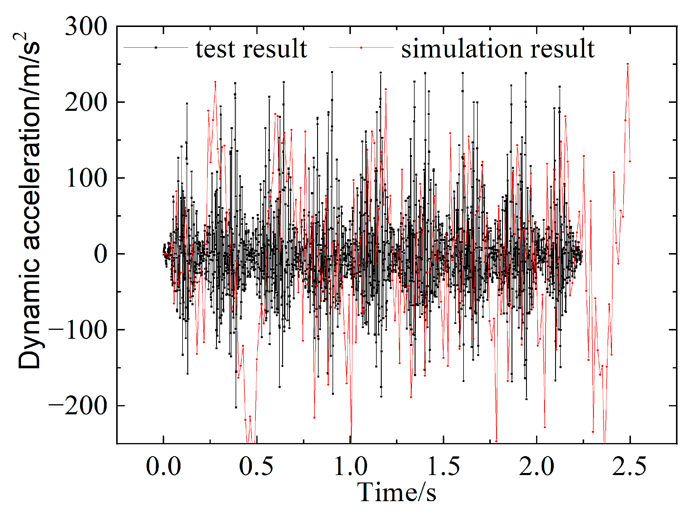
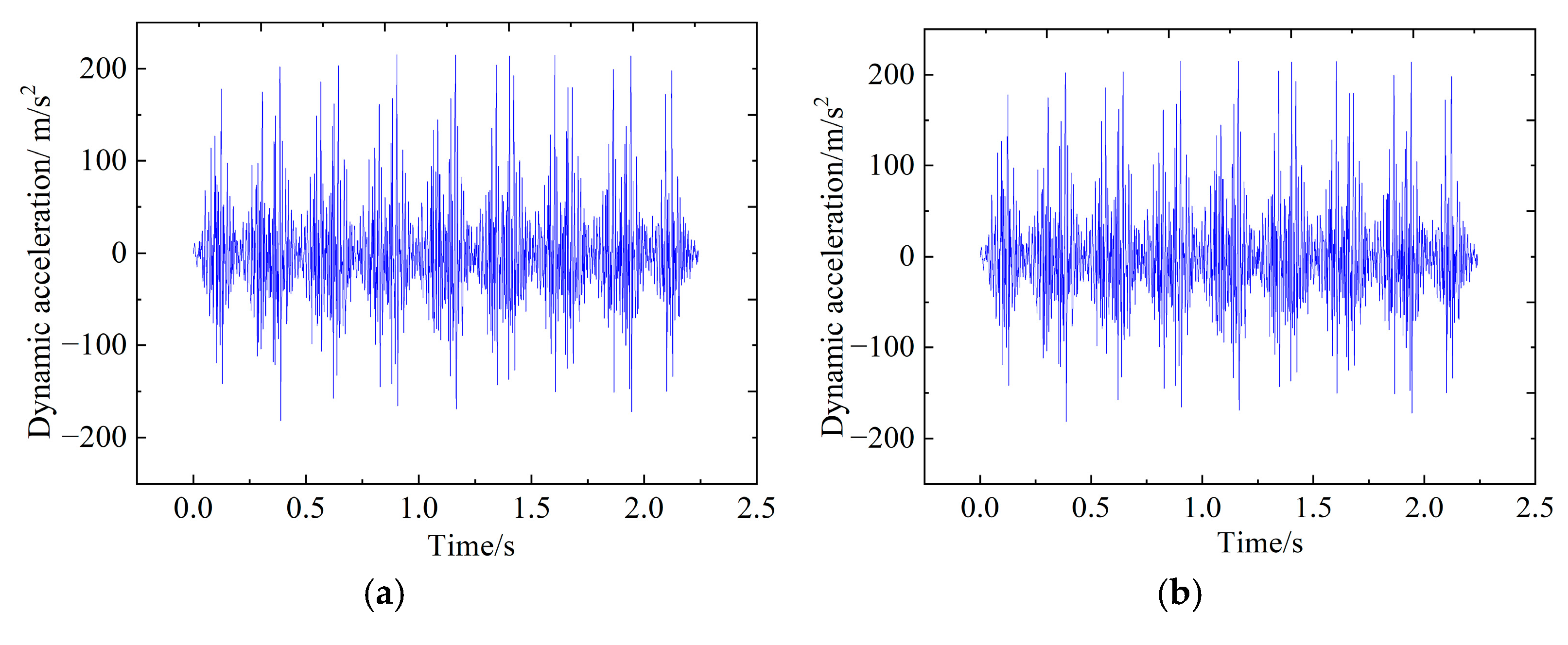
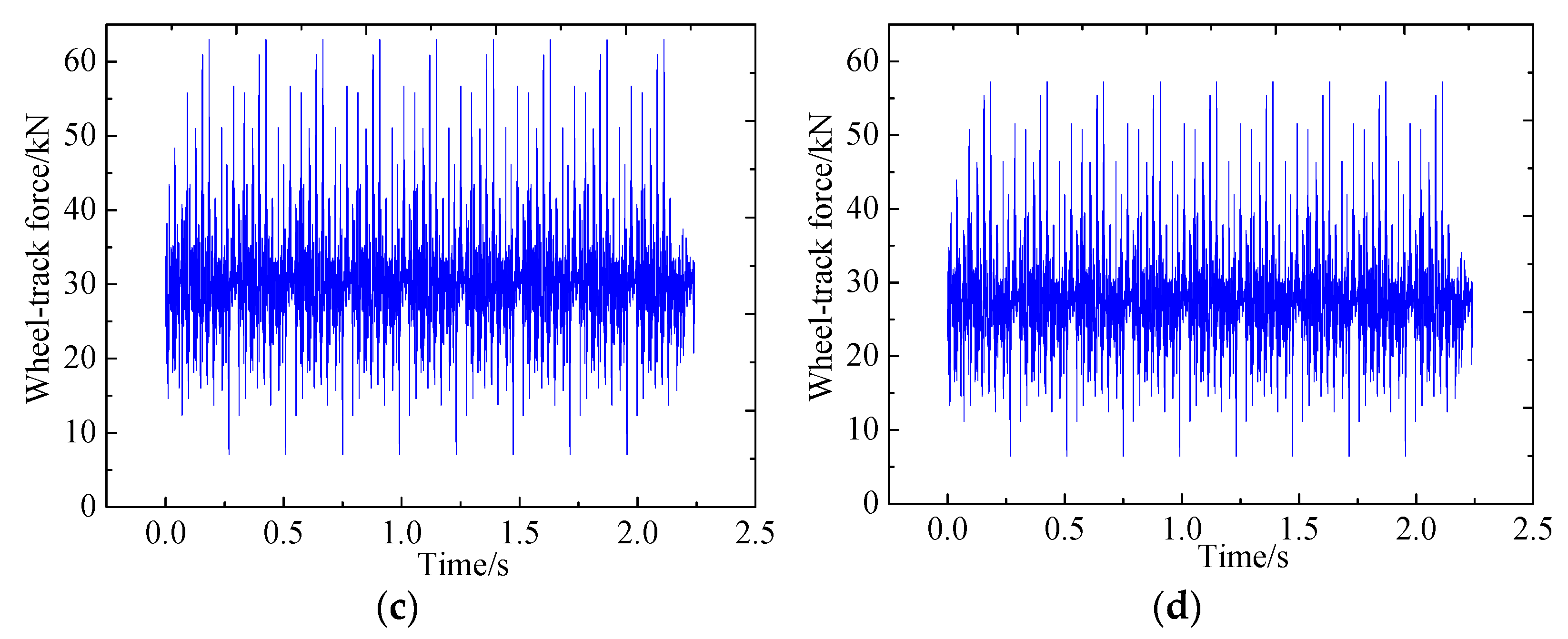
4.1. Time–History Curves

Figure 2 compares the calculated rail acceleration time–history curve with the test results. Figure 13 presents the calculated time–history dynamic responses at a train speed of 350 km/h on a bed surface. The figures reveal that the peaks correspond to the dynamic responses when the wheel passes the section, while the troughs correspond to the dynamic responses when the wheel has passed the section. A bogie passing is equivalent to two times the load and unload. The dynamic response begins to increase following a reduction when the front axle of the bogie passes the rail. This is the superposition result of the front and rear axle load acting on the roadbed. Moreover, the dynamic response is small when the front wheel passes and large when the rear wheel passes.
The natural frequency of the measured bed surface is determined as 21 Hz, while the second order frequency of the finite element model is 21.46 Hz, which is very close to the measured natural frequency. These results prove the reliability of the model.
The subgrade is observed to vibrate and overcome the damping of the subgrade soil under the action of the moving loads. As the depth increases, the vertical dynamic displacement, velocity and acceleration diffuse and attenuate, namely, the incidence of waves refraction, energy dissipation at different material interfaces. The vertical dynamic displacement, dynamic velocity, dynamic acceleration and dynamic stress on the rail surface rapidly decay after passing through the pads, fasteners, rail plates, etc. Furthermore, the dynamic elastic strain does not decrease with the increasing depth.
The mechanical properties of the interface between the graded crushed stone and the grade A and B filling layers change suddenly and intermittently. The vertical stress mutates 10 times from the concrete layer to the bed layer. In the above numerical calculation, the elastic modulus of graded crushed stone is about 3.68 times that of the group A and B fillers. Thus, the abrupt change in stress on the interface is not only related to the different elastic modulus, but also to the interface strain on both sides of the material. Stress and strain discontinuities also exist at the interfaces of other materials. The stress discontinuities with an equal magnitude are related to the constitutive properties and strain at both sides of the material. Furthermore, due to the damping effect, the train load dissipates energy in the form of a deeply propagated dynamic wave. Therefore, the dynamic stress attenuates with the increase in depth. The results also confirm this conclusion.

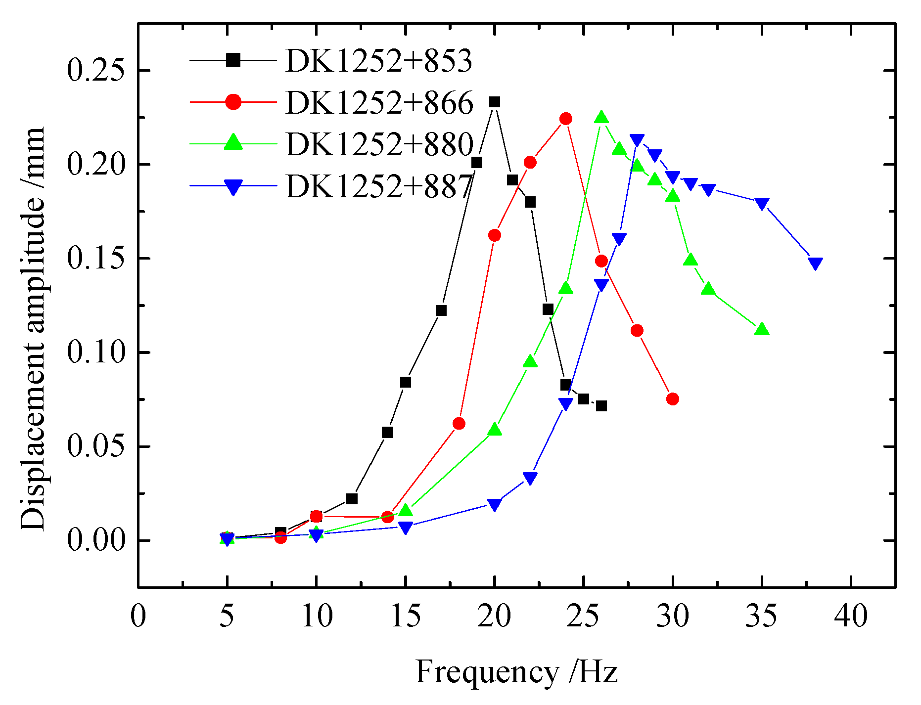
4.2. Frequency Domain

Modal analysis was performed to obtain the calculated frequency. The first vertical mode is 16.85 Hz, and the second vertical mode is 21.46 Hz (Figure 14).
The measured frequency was also tested with the excitation and pulse experiments according to the Code for the Measurement Methods of the Dynamic Properties of Subsoil using the test equipment described in Section 2.2. Here, we focus on the transverse frequency of the subgrade, and thus the transverse “resonance” frequency was analyzed and compared with the simulation data via maximum entropy analysis. Table 6 reports the obtained power spectra. The frequencies of the pulse method in sections DK1252 + 887 and DK1252 + 880 were 21 Hz and 22 Hz, respectively, with a maximum relative error below 5%. The peak frequency of the excitation method was 20 Hz, with a maximum relative error of less than 10%. Therefore, the subgrade natural frequency can essentially be determined as 21 Hz.

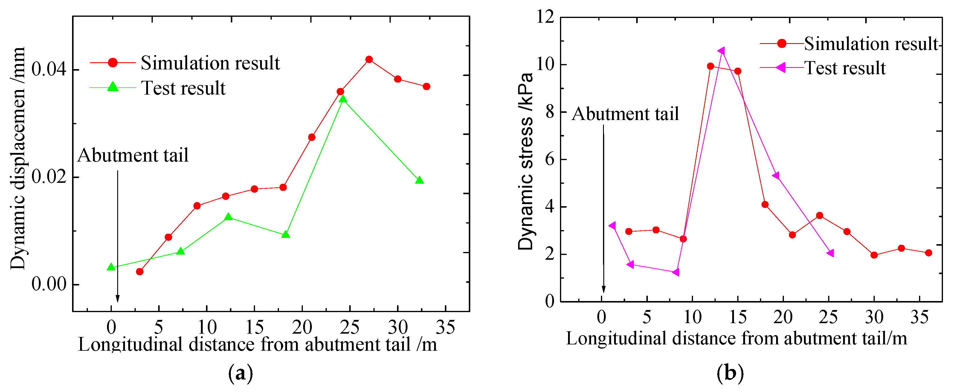
4.3. Comparison with Test Results

To further verify the accuracy of the simulation model, the simulation results were compared with the test dynamic displacements and stresses. Figure 15 compares the measured and simulated results of the dynamic displacement and stress on a bed surface at 350 km/s. The simulation results generally agree with the test results. In particular, the simulation stress determined in this paper is at the same order of magnitude as the stress reported in the literature [2], with a dynamic stress at the surface layer equal to 15.63 kPa. The slightly lower stress values obtained in this work compared to those in the literature [2] may be attributed to the distinct parameters used in the two models.

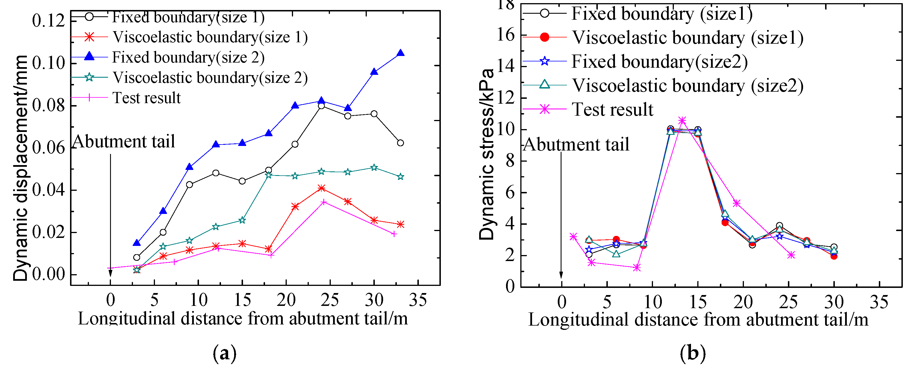
4.4. Comparison of Different Modeling Methods

Figure 16 compares the measured results with calculated dynamic displacement and stress with different boundaries and modeling sizes on a bed surface at 350 km/s. Figure 17 reveals the calculated dynamic stress values to be in general agreement across boundary treatment methods and model sizes, and the variation law is essentially consistent with the measured dynamic stress. However, the dynamic displacement varies with the boundary treatment method and model size, and it is evident that the calculated dynamic displacement considering a viscoelastic artificial boundary is closest to the measured value. This indicates that the viscoelastic artificial boundary not only absorbs the energy of the wave at the boundary of the model well, but also greatly reduces the size of the model and increases the speed of the computer.
Figure 18a compares the simulated and test results of dynamic stress with and without structural damping. The calculated results with added structural damping are closer to the measured results. This is because the dynamic stress is consistently attenuated along the depth of the subgrade. However, the attenuation degree of the calculated results is less than the mean. Figure 18b compares the simulated and test results of the dynamic stress under different CA models. It is more practical to simulate CA mortar with the spring-damping and shell elements. This is mainly reflected in the dynamic stress of the bed surface. The addition of the spring-damping unit can simulate the damping property of the CA mortar. The dynamic stress simulated by the two methods differs by 2 kPa, while the dynamic stress changes under the bed surface are consistent.
Figure 18c compares the simulated and test results of dynamic stress amplitude under different train load modeling methods. The results calculated with the deterministic load are closer to the test results compared to those of the other loads.

5. Discussion

In order to determine the comprehensive deformation modulus of a multi-layer foundation, it is necessary to calculate the deformation modulus of each soil layer and weight it according to the thickness of the soil layer. This process can be described as
E d m = i = 1 k h i E i / i = 1 k h i ,
where Edm is the comprehensive deformation modulus of the multi-layer foundation, Ei is the deformation modulus of each soil layer, and hi is the thickness of the soil layer. The comprehensive shear modulus Gdm is calculated using the same approach.
Based on the cross-hole test, the Edm of graded crushed stone + 5% cement, graded crushed stone, and group A and B fillers were determined as 1923.0 MPa, 695.80 MPa and 521.33 MPa, respectively, and the Gdm as 748.26 MPa, 262.84 MPa and 194.73 MPa, respectively.
Based on the lower hole test, the Edm of graded crushed stone + 5% cement, graded crushed stone and group A and B fillers was determined as 1856.55 MPa, 652.18 MPa and 498.93 MPa, respectively, and the Gdm as 726.81 MPa, 245.73 MPa and 186.40 MPa, respectively.

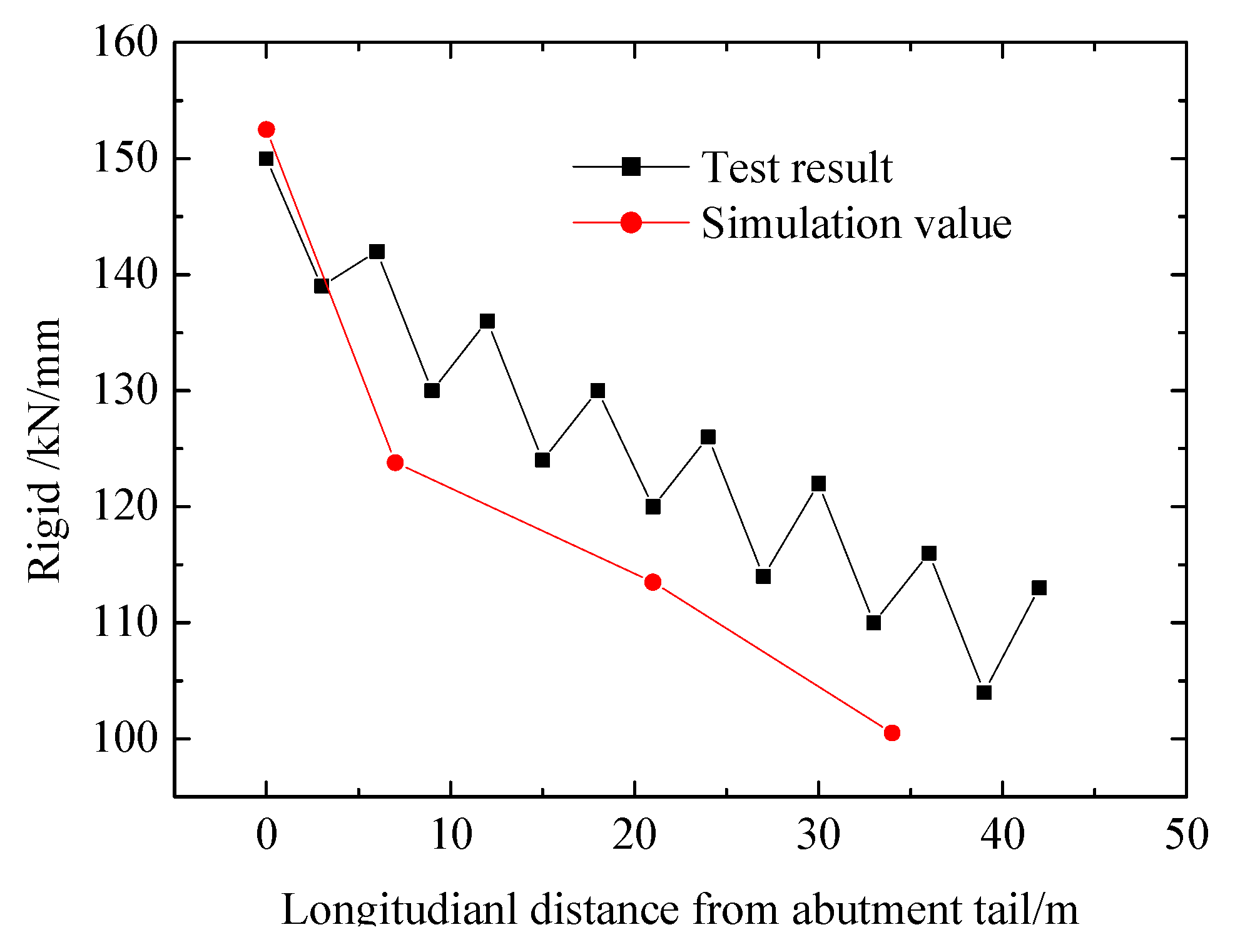
5.1. Variation Law of Stiffness along the Transition Section

In order to explore the variation laws of stiffness and modulus along the transition section, numerous scholars have investigated the overall modulus of the cross-section, principally using tests. In this paper, we obtained the comprehensive deformation modulus and rigid via simulations and tests (Table 7).
Figure 19 compares the experimental and simulated stiffness. Through simulation analysis, the stiffness of the bridge abutment and roadbed were determined as 150 kN/mm and 95 kN/mm, respectively, with the former just 1.58 times greater than the latter. The stiffness change rate from the bridge abutment to the roadbed through the transition section was calculated as 1.18 kN/mm/m. The variation trend of the comprehensive stiffness at the track with the distance from the bridge abutment is essentially consistent with the experimental results, and the calculated value is slightly smaller than the experimental value. This validates the results of the simulation model. These results are generally consistent with the design requirements, namely, the stiffness ratio of the bridge to the road should not exceed 2. This difference can essentially eliminate the impact of structural mutations, allowing the stiffness of the roadbed structure to transition more evenly. Furthermore, the deflection of the roadbed under wheel load tends to be consistent, greatly improving the service level and driving quality of the bridgehead pavement.
Through the excitation and cross-hole method tests, and based on the actual structural dimensions, the comprehensive modulus of the bridge abutment and roadbed were determined as 2001.16 MPa and 605.55 MPa, respectively, with the former only 3.3 times that of the latter. The change rate of the comprehensive elastic modulus from the bridge abutment to the roadbed through the transition section was 41 MPa/m. The stiffness of the bridge abutment and the roadbed were calculated as 152.72 kN/mm and 100.5 kN/mm, respectively, with the former just 1.52 times that of the latter. The stiffness change rate from the bridge abutment to the roadbed through the transition section was 1.53 kN/mm/m.
The excitation test results are clearly in good agreement with the simulation results. However, the results of the wave velocity test are relatively large, and the comprehensive modulus ratio of the transition section is determined as 3.3. Although this is also within the limit design value of the transition section, the calculation accuracy of the results requires further work.

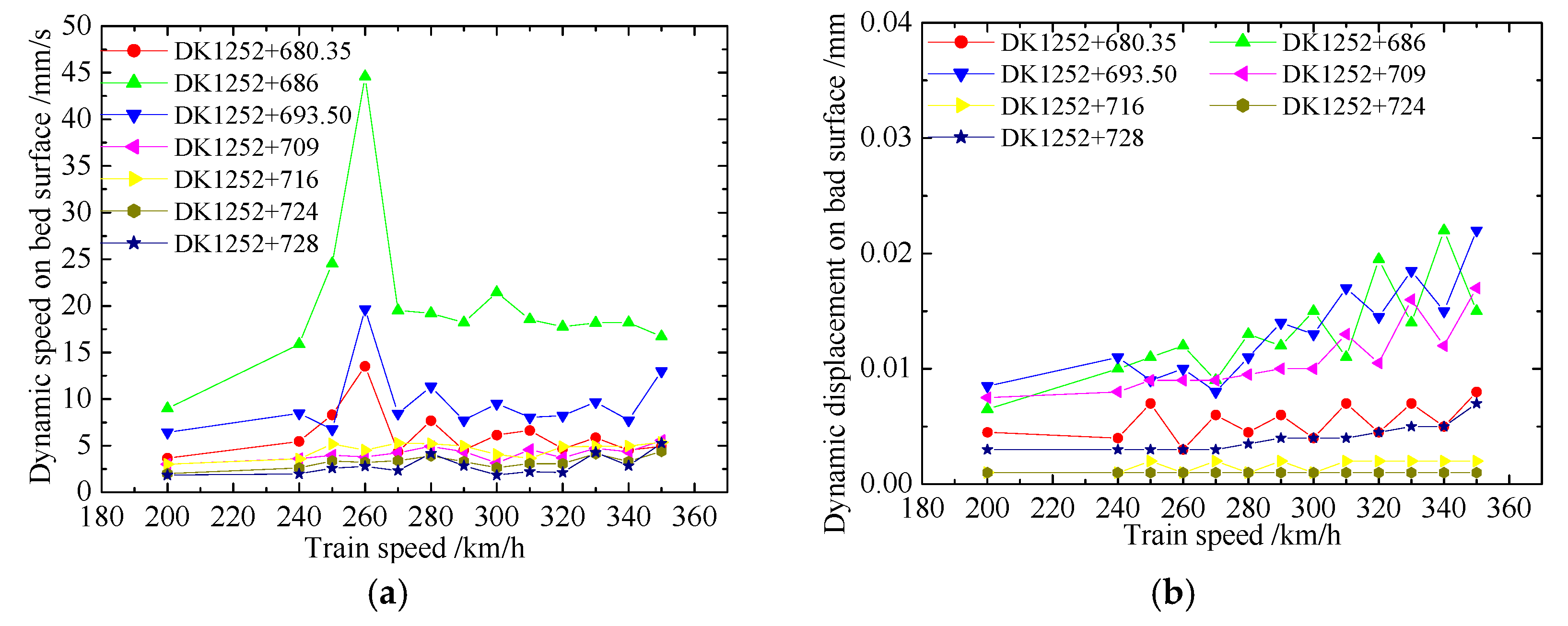
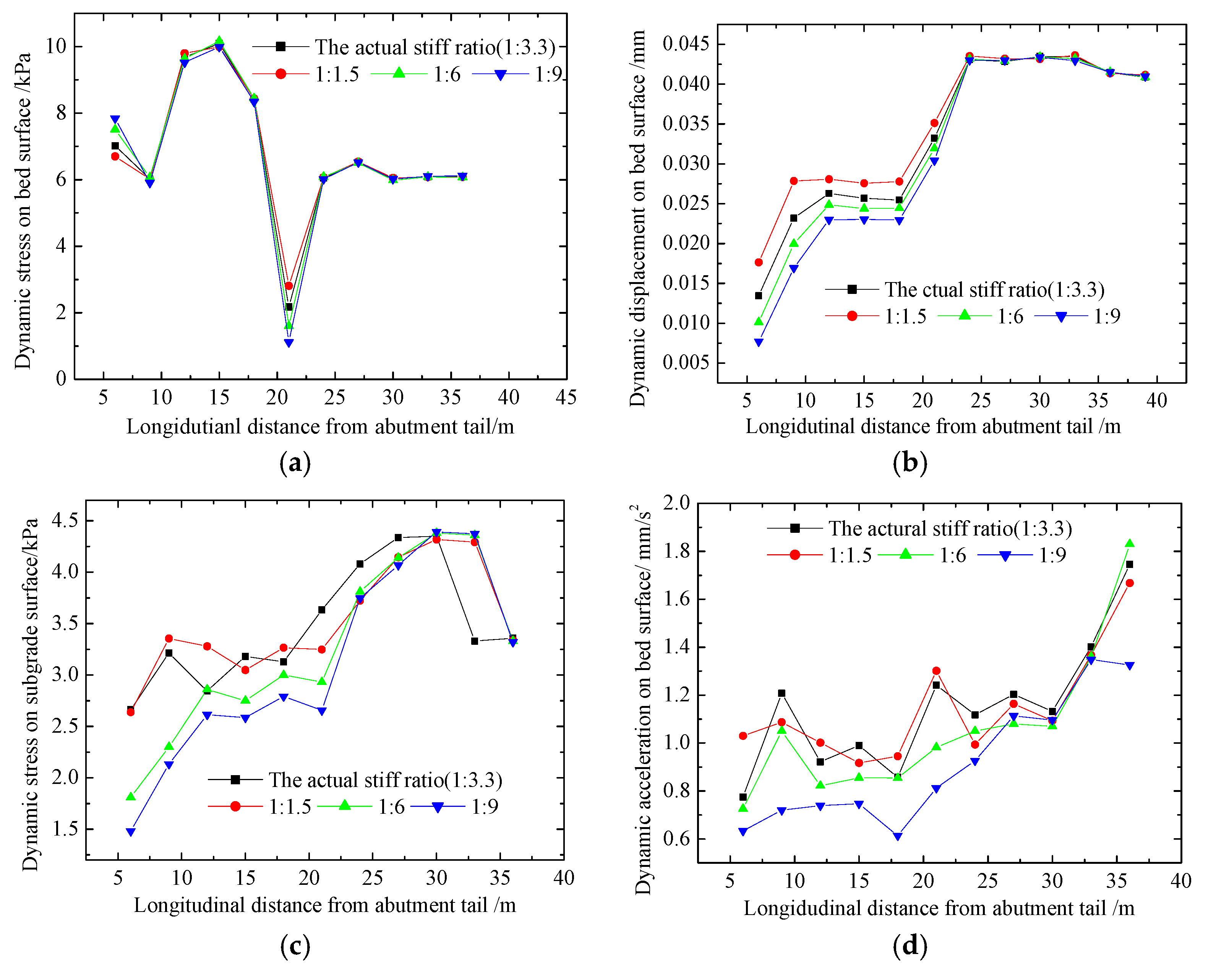
5.2. Analysis of the Influence of Transition Section Stiffness on Roadbed Dynamics

In order to explore the influence of the transition section stiffness ratio on the dynamic response of the transition, in the following, we only considered the stiffness irregularities in the simulation. In particular, the maximum amplitude of the actual road bridge transition section (stiffness ratio 1:3.3) and the stiffness ratios 1:1.5, 1:6 and 1:9 were compared and analyzed. Note that the stiffness of the ordinary roadbed remained unchanged, but the stiffness of the transition section increased. Table 8 reports the maximum amplitude calculated along the transition based on a 350 km/h-train speed, 0-rail surface-bending, 0-differential settlement, 20 m-transition length and a regular trapezoid-transition section. Figure 20 shows the variation curves of the dynamic parameters along the longitudinal distance at the tail of Wuhan station.
Table 8 reveals that the maximum amplitude of the dynamics do not vary greatly with the stiffness. However, the longitudinal variation characteristics exhibit substantial variation, particularly in the transition section. The greater the stiffness ratio, the smaller the dynamic displacement of the bed surface, yet the opposite is observed for the stress. This may be because the rigidity is the direct result of the displacement. This indicates that the difference in the stiffness of the structures at both ends of the transition section does not have a significant impact on the train passing the transition section. The on-site investigation of the status of the road bridge transition section also revealed that as long as the track is regularly lifted and repaired with ballast, and the track surface is kept smooth, the track inspection car can pass smoothly without the deduction of points.
Figure 20 shows that that the closer to the bridge, the greater the change in the dynamic response with the stiffness ratio. For the cross-section far from the transition section, the dynamic response is almost unaffected by the stiffness ratio, with 25 m determined as the boundary point.
In the bridge approach, as the rigid ratio increases, the dynamic responses change sharply along the longitudinal distance. When the stiffness ratio is greater than 1:6, these parameters increase more significantly, yet they do not exceed the standard value. Therefore, it is recommended to control the stiffness ratio of the transition section within 1:6 from the stationarity underneath.

6. Conclusions

In this paper, indoor and in situ tests were conducted to obtain the basic and stiffness index, providing parameters for the FEM and revealing the stiffness change law along the bridge approach. An effective track-subgrade FEM induced by a high-speed train on a bridge approach zone was then established by simplifying the train load, processing the boundary, and exploring the solutions of the constraint equations constrained by different elements.
The FEM proved to be effective by simplifying the train action and applying artificial boundaries. Future research will focus on improving the simulation of the dynamic effects of trains and the long-term interaction between trains and tracks. The comprehensive stiffness method can effectively explore the stiffness of a whole section, and this method can be adapted and improved to reflect the stiffness characteristic of a complex cross-section. Moreover, the stiffness and dynamic characteristics of the bridge approach are critical in the transition zone of high-speed railways, and the long term stability of the transition should be a focal point in design and management decisions.
Based on the results of this paper, we have made the following conclusions:
(1)
The calculated results of the time–history characteristics and dynamic changes along the longitudinal direction coincided with the test results, with the calculated and test natural frequencies determined as 21.46 Hz and 21 Hz (20 Hz or 22 Hz), respectively. This proves the reliability of the dynamic calculation model.
(2)
The difference between the wheel–rail force determined by the measured rail acceleration and the vertical wheel–rail force measured via ASTRI was less than 10%. This indicates that the is model more effective than establishing a whole vehicle-track-subgrade system.
(3)
The spring-damping and shell elements can simulate the damping property of the CA mortar better than the shell and board elements. Each type of element established and solved by the multi-point constraint equations produced strong connections and eliminated the additional stress generated using conventional methods.
(4)
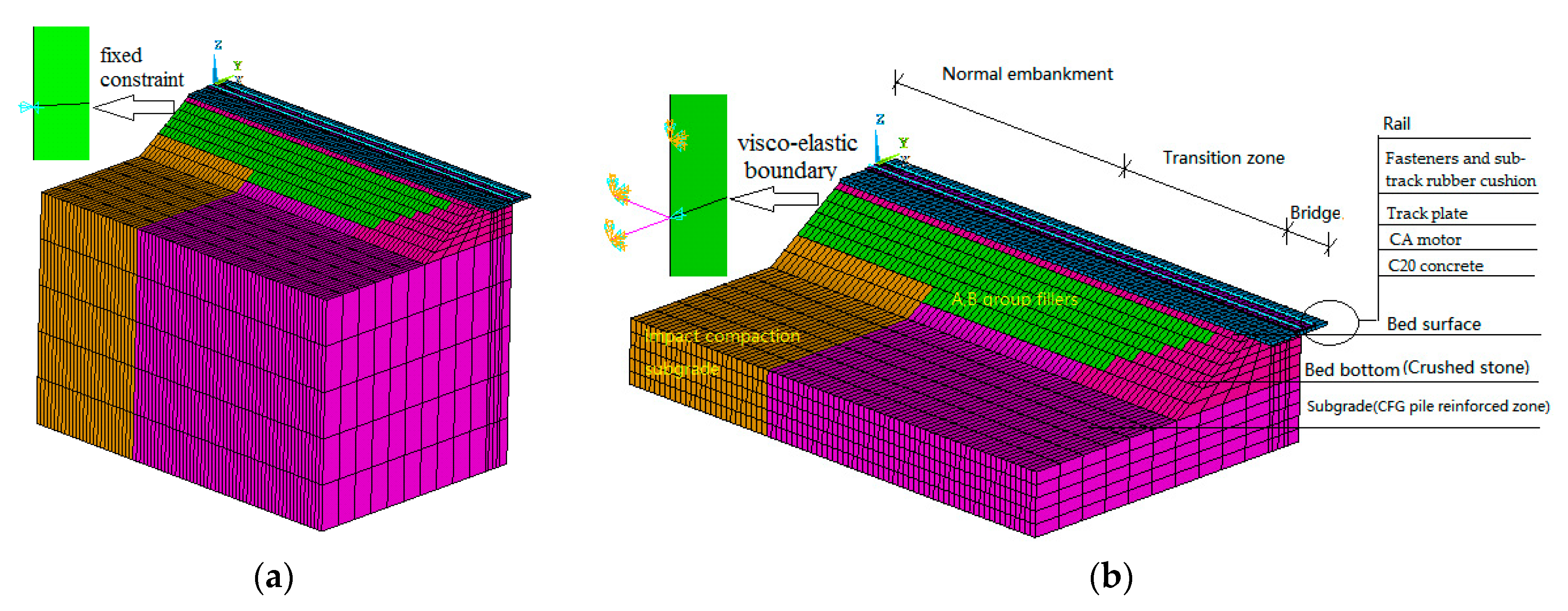
The viscoelastic artificial boundary-processing methods reduced the model size to one fifth of that of the model with fixed boundaries, and the calculation results were also closer to the test result than the calculation results with the fixed boundaries.
(5)
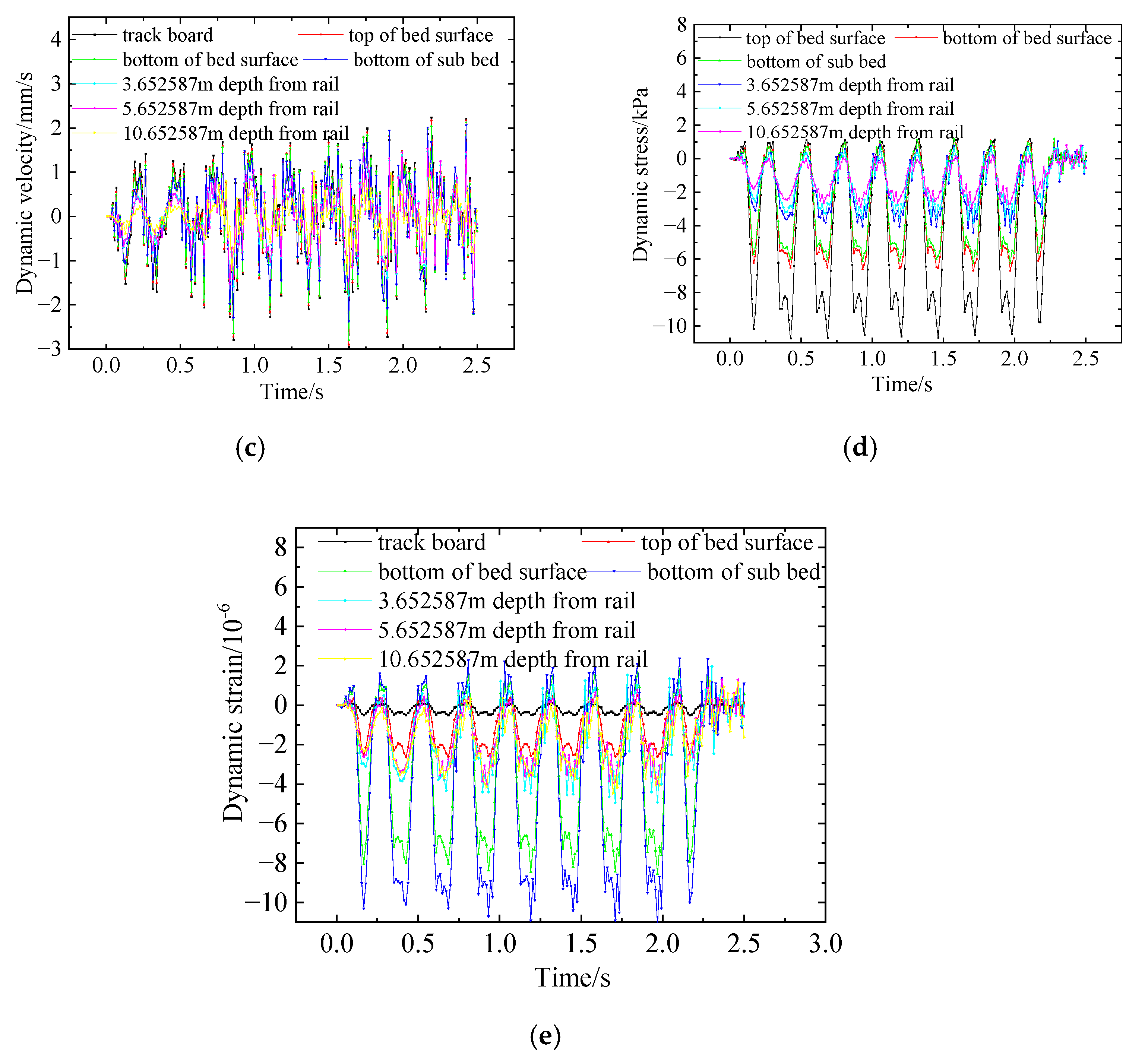
The numerical analysis shows that, under the train load, the vertical dynamic response at different depths of the same section is mainly attenuated from the surface of the bed to the bottom. Furthermore, the influence of the train load on the embankment is primarily reflected in the upper part of the structure. Consequently, the subgrade bed structure must be strengthened to ensure an effective HSR performance.

Author Contributions

Conceptualization, P.H.; methodology, W.L.; software, H.L.; validation, L.W. and H.L.; formal analysis, P.H. and W.G.; investigation, L.W., Y.W. and W.L.; resources, P.H. and W.G.; data curation, W.L.; writing—original draft preparation, P.H. and W.L.; writing—review and editing, P.H. and W.L.; visualization, P.H.; supervision, W.G.; funding acquisition, P.H. and W.G. All authors have read and agreed to the published version of the manuscript.

Funding

This research was funded by the National Natural Science Foundation of China (No. 50678177), and Excellent Youth Fund of Hunan Provincial Department of Education (Funder: Ping Hu; No. 20B098). National University Student Innovation and Entrepreneurship Project (S202311532014, S202111532023, S202111532015).

Data Availability Statement

The data presented in this study may be available on reasonable request from the first or corresponding author.

Conflicts of Interest

The authors declare no conflict of interest.

References

  1. Moliner, E.; Martínez-Rodrigo, M.D.; Museros, P. Dynamic performance of existing double track railway bridges at resonance with the increase of the operational line speed. Eng. Struct. 2017, 132, 98–109. [Google Scholar] [CrossRef]
  2. Shan, Y.; Shu, Y.; Zhou, S. Finite-infinite element coupled analysis on the influence of material parameters on the dynamic properties of transition zones. Constr. Build. Mater. 2017, 148, 548–558. [Google Scholar] [CrossRef]
  3. Shan, Y.; Albers, B.; Savidi, S.A. Influence of different transition zones on the dynamic response of track-subgrade systems. Comput. Geotech. 2013, 48, 21–28. [Google Scholar] [CrossRef]
  4. Bian, X.; Jiang, H.; Chang, C.; Hu, J.; Chen, Y. Track and ground vibrations generated by high-speed train running on ballastless railway with excitation of vertical track irregularities. Soil Dyn. Earthq. Eng. 2015, 76, 29–43. [Google Scholar] [CrossRef]
  5. Ribeiro, C.A.; Calçada, R.; Delgado, R. Experimental assessment of the dynamic behaviour of the train-track system at a culvert transition zone. Eng. Struct. 2017, 138, 215–228. [Google Scholar] [CrossRef]
  6. Zhai, W. Train-Rail Coupling Dynamics, 4th ed.; Railway Press: Beijing, China, 2016. [Google Scholar]
  7. Bebianoa, R.; Calçadab, R.; Camotima, D.; Silvestre, N. Dynamic analysis of high-speed railway bridge decks using generalised beam theory. Thin-Walled Struct. 2017, 114, 22–31. [Google Scholar] [CrossRef]
  8. Sheng, X.; Zhon, T.; Li, Y. Vibration and sound radiation of slab high-speed railway tracks subject to a moving harmonic load. J. Sound Vib. 2017, 395, 160–186. [Google Scholar] [CrossRef]
  9. Chai, J.C.; Shrestha, S.; Hino, T.; Ding, W.Q.; Kamo, Y.; Carter, J. 2D and 3D Analyses of an Embankment on Clay Improved by Soil-Cement Columns. Comput. Geotech. 2015, 68, 28–37. [Google Scholar] [CrossRef]
  10. Berggren, E. Railway Track Stiffness. Dynamic Measurements and Evaluation for Efficient Maintenance. Division of Rail Vehicles; Royal Institute of Technology (KTH): Stockholm, Sweden, 2009. [Google Scholar]
  11. TB10102-2010; Code for Soil Test of Railway Engineering. China Railway Publishing House: Beijing, China, 2010.
  12. Madshus, C.; Kaynia, A.M. High-speed railway lines on soft ground: Dynamic behaviour at critical train speed. J. Sound Vib. 2000, 231, 689–701. [Google Scholar] [CrossRef]
  13. Galvín, P.; Domínguez, J. Experimental and numerical analyses of vibrations induced by high-speed trains on the Córdoba-Málaga line. Soil Dyn. Earthq. Eng. 2009, 29, 641–657. [Google Scholar] [CrossRef]
  14. Costa, P.A.; Calçada, R.; Cardoso, A.S. Track-ground vibrations induced by railway traffic: In-situ measurements and validation of a 2.5D FEM-BEM model. Soil Dyn. Earthquak Eng. 2012, 32, 111–128. [Google Scholar] [CrossRef]
  15. Shan, Y.; Zhou, S.; Shu, Y. Differential Settlement and Soil Dynamic Stress of a Culvert-embankment Transition Zone Due to an Adjacent Shield Tunnel Construction. KSCE J. Civ. Eng. 2018, 22, 2325–2333. [Google Scholar] [CrossRef]
  16. Hu, P.; Zhang, C.; Chen, S.; Wang, Y.; Wang, W.; Duan, W. Dynamic responses of bridge–embankment transitions in high speed railway: Field tests and data analyses. Eng. Struct. 2018, 175, 565–576. [Google Scholar] [CrossRef]
  17. Dürrwang, R.; Hotz, C.; Schulz, G. Erfahrungen mit dem Erdbaukonzept ARCADIS-Messungen unter Verkehr. EI-Der Eisenbahningenieur 2005, 1, 24–31. [Google Scholar]
  18. Bonopera, M.; Liao, W.C.; Perceka, W. Experimental-theoretical investigation of the short-term vibration response of uncracked prestressed concrete members under long-age conditions. Structures 2022, 35, 260–273. [Google Scholar] [CrossRef]
  19. Wang, T.H.; Huang, R.; Wang, T.W. The variation of flexural rigidity for post-tensioned prestressed concrete beams. J. Mar. Sci. Technol. 2013, 21, 300–308. [Google Scholar]
  20. Heydari-Noghabi, H.; Varandas, J.N.; Esmaeili, M.; Zakeri, J. Investigating the Influence of Auxiliary Rails on Dynamic Behavior of Railway Transition Zone by a 3D Train-Track Interaction Model. Lat. Am. J. Solids Struct. 2017, 14, 2000–2018. [Google Scholar] [CrossRef]
  21. Fu, Q.; Wu, Y. Three-dimensional finite element modelling and dynamic response analysis of track-embankment-ground system subjected to high-speed train moving loads. Geomech. Eng. 2019, 19, 241–254. [Google Scholar]
  22. Germonpré, M.; Degrande, G.; Lombaert, G. A track model for railway-induced ground vibration resulting from a transition zone. Proc. Inst. Mech. Eng. Part F J. Rail Rapid Transit 2018, 232, 1703–1717. [Google Scholar] [CrossRef]
  23. Chen, M.; Sun, Y.; Zhai, W. High efficient dynamic analysis of vehicle-track-subgrade vertical interaction based on Green function method. Vechicle Syst. Dyn. 2019, 58, 1076–1100. [Google Scholar] [CrossRef]
  24. GB/T 50269-2015; Code for Measurement Methods of Dynamic Properties of Subsoil. Planning Press: Beijing, China, 2015. (In Chinese)
  25. Li, D.; Davis, D. Transition of railroad bridge approaches. J. Geotech. Geoenviron. Eng. ASCE 2005, 131, 1392–1398. [Google Scholar] [CrossRef]
  26. Nakasone, Y.; Yoshimoto, S.; Stolarski, T.A. Engineering Analysis with ANSYS; Elsevier: Amsterdam, The Netherlands, 2011; 480p. [Google Scholar]
  27. Dewu, L. A deterministic analysis of dynamic train loading. J. Gansu Sci. 1998, 10, 25–29. (In Chinese) [Google Scholar]
  28. Sun, S.C. Theoretical Research on Wheel/Rail Contact Force Identification and Its Application. Ph.D. Thesis, Railway Academy, Beijing, China, 2016. (In Chinese). [Google Scholar]
  29. Hu, P.; Zhang, C.; Wen, S.; Wang, Y. Dynamic responses of high-speed railway transition zone with various subgrade fillings. Comput. Geotech. 2019, 108, 17–26. [Google Scholar] [CrossRef]
  30. TB 10001—2016; National Railway Administration of the People’s Republic of China. Code for Design of Railway Earth Structure. Railway Publishing House: Beijing, China, 2017.
Figure 1. Longitudinal section of bridge approach.
Mathematics 11 04202 g001
Figure 2. Comparison of the distance–history between the simulation results and the measured data.
Mathematics 11 04202 g002
Figure 3. Schematic diagram of the drilling arrangement used for the tests.
Mathematics 11 04202 g003
Figure 4. Principle of the excitation method tests. (Note: Kz is the compressive stiffness of the foundation and foundation (kN/m), m is the total mass of the vertical vibration of the foundation kg), ζ z is vertical damping ratio of foundation; P(t) is excitation force.).
Mathematics 11 04202 g004
Figure 5. Amplitude–frequency response curves of in bridge approach.
Mathematics 11 04202 g005
Figure 6. 3D bridge approach simulation model (a) Fixed boundary. (b) Viscoelastic artificial boundary.
Mathematics 11 04202 g006
Figure 7. Three-dimension viscoelastic artificial boundary.
Mathematics 11 04202 g007
Figure 8. Processing of deterministic load. (a) Time–history curve atDK1252 + 885 section. (b) Time–history curve at DK1252 + 863 section. (c) Wheel–track force at DK1252 + 885 section. (d) Wheel–track force at DK1252 + 863 section.
Mathematics 11 04202 g008aMathematics 11 04202 g008b
Figure 9. Diagram of dynamic load application.
Mathematics 11 04202 g009
Figure 10. Superposition of three forces on track.
Mathematics 11 04202 g010
Figure 11. Offset connection between beam axis and spring element.
Mathematics 11 04202 g011
Figure 13. Time–history curves on the bridge approach zone section. (a) Dynamic displacement. (b) Dynamic acceleration. (c) Dynamic speed. (d) Dynamic stress. (e) dynamic elastic strain.
Mathematics 11 04202 g013aMathematics 11 04202 g013b
Figure 14. First- and second-order modes in the bridge approach zone. (a) The first order (16.85 Hz). (b) The second order (21.46 Hz).
Mathematics 11 04202 g014
Figure 15. Comparison of measured dynamic results and simulation results. (a) Dynamic displacement. (b) Dynamic stress.
Mathematics 11 04202 g015
Figure 16. Comparison of measured dynamic results and simulation results with different boundaries. (a) Dynamic stress. (b) Dynamic acceleration.
Mathematics 11 04202 g016
Figure 17. Comparison of dynamic results with the results of different modeling methods. (a) Dynamic displacement. (b) Dynamic stress.
Mathematics 11 04202 g017
Figure 18. Comparison chart of dynamic results with different modeling methods. (a) Different damping. (b) Different CA motor. (c) Different moving load.
Mathematics 11 04202 g018
Figure 19. Comparison of measured and simulated stiffness values.
Mathematics 11 04202 g019
Figure 20. Variation curves of the dynamic parameters along the longitudinal distance at the tail of Wuhan station. (a) Dynamic stress on bed surface. (b) Dynamic displacement on bed surface. (c) Dynamic stress on subgrade. (d) Acceleration on bed surface.
Mathematics 11 04202 g020
Table 1. Results of wave speed tests in bridge approach.
SectionFilling MaterialDepth (m)Vcp/Vdp
(m/s)
Vcs/Vds
(m/s)
μcdEcd/Edd
(MPa)
Gcd/Gdd
(MPa)
+853A0.2968.2/948.2520.1/510.10.297/0.2961824.8/1754.1703.3/676.6
B1.2659.4/633.0320.3/305.00.346/0.349678.0/617.3252.4/228.8
2.2606.1/586.0319.0/300.00.308/0.322655.8/585.6250.3/221.4
C3.2620.6/607.0322.6/312.00.315/0.320574.7/539.9218.5/204.4
4.2593.3/580.5287.8/282.70.346/0.345468.3/451.3173.9/167.8
5.2591.8/573.6265.6/260.30.374/0.370407.1/390.0148.1/142.3
+880A0.2944.0/929.3526.4/519.20.274/0.2731837.8/1784.6720.5/700.9
B1.2636.7/623.2325.3/319.30.323/0.322689.0/663.1260.3/250.8
2.2663.2/654.6342.4/338.50.318/0.317760.4/742.7288.4/281.9
C3.2620.0/605.5307.5/300.80.337/0.336530.9/507.8198.6/190.0
4.2656.7/640.8323.0/315.90.340/0.339587.4/561.4219.1/209.6
5.2630.4/618.7316.3/311.90.332/0.330559.6/543.36210.1/204.3
+887A0.2975.3/961.8535.9/529.20.284/0.2831917.1/1868.3746.7/728.1
1.21004.7/991.9545.6/539.50.291/0.2901998.2/1952.3774.0/756.8
2.2998.8/978.5553.6/544.80.278/0.2752037.1/1968.4796.8/771.7
Note: “A” represent “Graded crush stone +5% cement”, “B” represent “Graded crush stone ”, “C” represent “Group A and B filler”. “Depth” means “Depth from bed surface”. The subscript “c” represents results from cross-hole test, The subscript “d” represents results from down-hole test.
Table 2. The stiffness and damping of the roadbed along the bridge approach.
SectionsDK1252 + 887DK1252 + 880DK1252 + 866DK1252 + 853
Kx (kN/mm)152.5123.8113.5100.5
Damping ratio0.0570.0660.0850.092
Table 3. Calculation model parameters of the tunnel–culvert–culvert transition section.
Parameters Elastic Modulus E (GPa)Poisson’s
Ratio ν
Density
ρ (kg/m3)
Internal Friction Angle Φ (°)Cohesion C (MPa)Elastic
Modulus (N/m3)
Damping (N•s/m2)
Structure and Material
Rail2100.37800 4.5 × 10⁵
Track plate (C50)35.00.16673000
CA motor layer0.0950.401800 1.25 × 1098.3 × 104
C20 concrete24.00.202700
Graded crushed stone + 5% cement1.89 *0.284 *2600 *40.0 *0.18 *
Graded crushed stone0.674 *0.326 *2560 *39.5 *0.16 *
A, B group filling0.510 *0.340 *2477 *41.8 *0.2 *
CFG Pile0.5340.242300
* The value obtained from tests are marked with an asterisk in the upper-right corner.
Table 4. Dynamic load of simulation values and measured values.
PositionTransition SectionEmbankment
Deterministic method (kN)6357
Test results of ASTRI (kN)65.563.3 (curved embankment)
Percentage difference (%)3.8%9.9%
Table 5. Elements and dimensions of the model.
StructuresElementDimensions and Others
RailBEAM188The length of the bridge approach is 58.2 m, the length of the bridge pier is 6.0 m, the track gauge is 1.435 m, and the spacing between fasteners is 0.6 m.
Fasteners and sub-track rubber cushionSpring and damping element COMBIN14The distance between the track board and the top surface of the track is 212 mm, with a track height of 174 mm, a thickness of 2 mm for the iron pad under the track and a thickness of 10 mm for the rubber pad under the track
Track plate (C50)Shell element SHELL143 The surface of the track board is convex and concave ribbed, with a length of 5000 mm, a width of 2340 mm, a thickness of 190 mm, a notch radius of 280 mm, a protective layer thickness of 20 mm.
CA motor layerShell element SHELL143 and a spring damping elementInject material CA under the board, with a mortar layer thickness of 0.05 m and a width of 2.34 m.
C20 concreteSolid element SOLID45Take half of the road width, 4.3 + 2.5 = 6.8 m, with a thickness of 0.3 m
Bed surfaceSolid element SOLID45Take half the road width, with an upper width of 4.3 + 2.5 = 6.8 m, a lower width of 0.6 + 4.3 + 2.5 = 7.4 m, and a thickness of 0.4 m
Bed BottomSolid element SOLID45The slope ratio of the roadbed slope is 1:1.5, taking half of the road width, with a thickness of 0.75 m. The upper width is 0.6 + 4.3 + 2.5 = 7.4 m, and the lower width is 1.125 + 0.6 + 4.3 + 2.5 = 8.525 m
Table 6. Comparative analysis of natural frequency.
Test MethodsTest SectionNatural Frequency/HzMaximum Relative Error
Excitation methodDK1252 + 8532010%
Pulse methodDK1252 + 887215%
DK1252 + 88022
Table 7. Comparison of stiffness in different methods and positions.
IndexBridgeSubgrade MultipleRate of Change
Comprehensive deformation modulus2001.16 MPa605.55 MPa3.341 MPa/m
Rigid by test152.72 kN/mm100.5 kN/mm1.521.53 kN/mm/m
Rigid by simulation150 kN/mm95 kN/mm1.581.18 kN/mm/m
Note: ① the comprehensive modulus of each cross sections is obtained by conducting wave velocity testing and using the comprehensive stiffness algorithm (Section 2.3 and Section 5); ② The stiffness values of each cross section is calculated through the excitation method test (Section 2.4); ③ Approximate dynamic stiffness of each section is obtained by using the rail wheel rail force by rail surface dynamic displacement, which calculated in simulation model in Section 5.
Table 8. The influence of transition stiffness on the peak values on various dynamic parameters.
Stiffness RationAcceleration/m/s2Stress/kPaDisplacement/mm
a r a b σ b σ s 1 σ s 2 U r U s 1
1:1.5279.332.0110.849.994.321.720.045
1:3.3279.281.8611.1710.094.341.720.043
1:6279.301.8711.4210.164.381.720.043
1:9279.291.9111.399.994.391.720.043
Note: “stiffness ratio” refers to the ratio of the stiffness of the transition section to the comprehensive modulus of the ordinary. a r —acceleration on rail, a p —acceleration on plate, σ s 1 —stress on bed surface, σ s 2 —stress on subgrade surface, U r —displacement on rail, U s 1 —displacement on bed surface.
Disclaimer/Publisher’s Note: The statements, opinions and data contained in all publications are solely those of the individual author(s) and contributor(s) and not of MDPI and/or the editor(s). MDPI and/or the editor(s) disclaim responsibility for any injury to people or property resulting from any ideas, methods, instructions or products referred to in the content.

