Abstract
In this article, we study ovals of constant width in a plane, comparing them to particular circles. We use the vertices on the oval, after counting them, as a reference to measure the length of the curve between opposite points. A new proof of Barbier’s theorem is introduced. A distance function from the origin to the points of the oval is introduced, and it is shown that extreme values of the distance function occur at the vertices and opposite points. Comparisons are made between ovals and particular circles. We prove that the differences in the distances from the origin between the particular circles and the ovals are small and within a certain range. We also prove that all types of ovals described in this paper are analytically and geometrically enclosed between two defined circles centered at the origin.
MSC:
52A10; 53A04; 53C80
1. Introduction
An oval is a smooth closed convex curve in . Two points on an oval are opposite if their tangent lines are parallel. An oval is a curve of constant width if the perpendicular distance between tangent lines at opposite points is constant [1]. Al-Banawi [2] studied the geometry of ovals in using the support function. The support function measures the perpendicular distance from the tangent line at a point on the oval to the origin [3]. Al-Banawi [2] gave a parametrization for an oval using the support function, and deduced other results using the support function regarding the curve of the focal points of the function that represents the oval and the length of the curve itself.
Al-Banawi and Al-Btoush [4] used the Fourier-series expansion of the support function to count the extreme points on a curve of constant width and established a formula for the area enclosed within the oval in terms of the support function itself. In [5], Resnikoff also used the Fourier series to derive the properties of ovals of constant width in .
In this study, we established new theorems regarding such extreme values, and we connected them to the half-length of the oval as they represent the maximum values of the curvature. Our oval is a generalization of the curve introduced by Fillmore [6].
Al-Banawi and Jaradat [7] produced a model for the width of an oval in using a linear second-order ordinary differential equation with constant coefficients, showing that opposite points on a curve of constant width have the same focal points, and the affine normal lines coincide.
The work described in this paper is supported by the idea that continuous ovals of constant width have approximations, an idea that was presented by Tanno [8]. Whereas Tanno assumed that the parametrization of the oval is a continuous differential curve in , Wegner [9] produced an analytic approximation for such ovals of constant width. Tanno [8] proved that for any positive number , the neighborhood of a continuous oval of constant width contains a -oval of the same constant width. Wegner [9] showed that such an approximation is real and analytic by simplifying the proof provided by Tanno using the support function.
Fu and Zhou [10] used the characteristic equation of a time delay system to analyze a smooth curve of constant width. Fu and Zhou presented the simulation results regarding the influence of the derivative orders on a smooth noncircular curve of constant width. A hypothesis [10] aimed to show that a circle is the only curve of constant width whose parametric equation is still a smooth curve of constant width after any number of derivatives.
In [6], Fillmore introduced a parametric formula of a curve of constant width with three vertices. Here, we generalize this formula to an odd number of vertices greater than three taking into account that Fillmore’s formula was joined by the shadow concept [11].
It should be mentioned here that our approach uses a clear parametric formula, which enables us to analyze and describe different ovals together. Our method supports the presentation of simulation results, which illustrate the theoretical analysis regarding the many properties of curves of constant width.
The remainder of this paper is structured as follows: In Section 2, we count the vertices on an oval of constant width. The vertices are points where the curvature of the oval is the maximum. Then, we measure the length of the oval between two opposite points. We also introduce a new proof of Barbier’s theorem. In Section 3, we measure the distance from the origin to any point on an oval of constant width. Our measurements include the general form parallel to special curves, which are circles. Also, we show that the maximum and minimum values occur at the vertices and opposite points of the oval. In Section 4, our results are supported by figures that show how circles are close to general curves of constant width with differences in curves lengths. Next, we compare ovals of constant width with a circle centered at the origin with radius and then with a circle that is not centered at the origin with radius a. Also, our graphs include a third comparison with two circles centered at the origin: one with a radius of and the other one with a radius of . Section 5 is our conclusions.
2. Ovals of Constant Width
In [2], it was proved that if f represents the oval and is the support function, then at , we have
Also, in [2], it was proved that the curvature of f at is given by
The work in this study was built on a formula that is a generalization of the formula introduced by Fillmore [6]. In fact, we build our study on the parametric function
where , , and n is an odd natural number, whereas in [6].
Our first result includes a parametrization of an oval of constant width with a sufficient condition for convexity. By convexity, we mean that the oval is positive everywhere. Geometrically, this means that at any point on the oval, the oval entirely lies on one side of the tangent at that point.
Theorem 1.
Consider a parametric function f defined by (1). Then, the image of f is an oval of constant width provided that .
Proof.
A tangent of f is given by
Since , we take as the unit tangent with length .
Now, ; so, is the opposite point of on the image of f.
Moreover, .
Hence, f is an oval of constant width . □
It is important to mention here that Theorem (1) provides us with the possible values of the odd number n, provided that a is determined. In fact, given a particular value of a, one can choose n such that .
In the geometry of plane curves, a vertex is a point at which the curvature has a local extreme value [12]. In our study, we followed the next definition.
Definition 1.
Let be the curvature of f at θ. Then, P is a vertex of the image of f if the curvature of f at P is the maximum.
Theorem 2.
Let f be an oval of constant width of the form (1). Then, f has n vertices, namely, at
Proof.
The second derivative of the function f is given by
Then, .
Hence, .
.
.
The maximum values of K occur at , while the other values correspond to the minimum values at opposite points. □
Theorem 3.
Consider the curve f given by (1). Then, the length L of the curve from a point on the curve at an angle θ to the point at the opposite angle is equal to
Proof.
Let ; then, the curve length from to is
□
The next theorem is known as Barbier’s theorem (1860), which was proved in [13]. Al-Banawi [2] introduced another proof using the support function. Our new proof here is a different version, as it uses the parametrization in (1).
Theorem 4.
Consider the curve f given by (1). Then, the total length L of the curve is equal to
Proof.
The calculation of the total length L of the curve f follows the same strategy as in the proof of Theorem (3), except that we integrate over the whole domain . That is,
□
Theorem 5.
Consider the curve f given by (1). Then, the length L of the curve from a vertex on the curve at an angle θ to the point at the opposite angle is equal to .
Proof.
Let , so that is a vertex on curve
Since, from Theorem (3), with ,
Then, . □
Theorem 6.
Consider the parametric curve f given by (1). Then, the length L of the curve from a vertex point on the curve to next one is given by , which is equal to the total length divided by the number of vertices.
Proof.
□
3. Distance from the Origin and Comparisons between Ovals and Particular Circles
In the next theorem, we determine the distance from the origin to any point on an oval defined by (1).
Theorem 7.
Consider the curve given by (1). Then, the distance function from the origin to a point on the curve at an angle θ is
Proof.
Using Pythagorean theorem, the distance from the origin to a point on the curve is given by
□
Corollary 1.
In a special case where , the distance from the origin to any point on the curve, , is , which means that the curve forms a circle centered at the origin, with radius .
Proof.
and
. Therefore,
which represents a circle centered at the origin with radius . □
Corollary 2.
In a special case where , the distance from the origin to any point on the curve,, is , which means that the curve forms a circle centered at with radius a.
Proof.
Substituting into the distance function defined by (2), , gives
Now, by substituting in (1), we obtain
and
; therefore,
Also, since we proved that , then
which represents a circle centered at with radius a. □
Corollary 3.
The distance function from the origin to the curve, given by Theorem (7), attains its maximum values at the vertices, namely, at
with a maximum value of . It attains its minimum values at the opposite points, namely, at
with a minimum value of .
Proof.
We have, from Theorem (7),
Then,
We need .
Since , then
; therefore,
Theorem 8.
Consider the curve given by (1). In the special case where , the difference between and is determined by
Proof.
We have
Then,
We need
Since , then
; therefore,
The minimum values of occur at the vertices , while other values correspond to the maximum values of opposite points.
The minimum value of is
The maximum value of is
Therefore, . □
Theorem 9.
Consider the curve given by (1) and the circle with radius centered at the origin. Then, the intersection points between the curve, for any value of n, and the circle occur at the vertices of the curve, namely, at
Proof.
Since and , then, to obtain the intersection points, we let
, so
Matching the coefficients on both sides gives
; therefore,
Also, from the matching, we have
therefore,
Taking the common values in both cases above, we obtain
which are the vertices of the curve. □
Theorem 10.
Consider the curve given by (1) and the circle with radius centered at the origin. Then, the intersection points between the curve for any value of n and the circle occur at the opposite points to the vertices of the curve, namely, at
Proof.
Since and , then, to obtain the intersection points, we let
, so
Matching the coefficients on both sides gives
; therefore,
Also, from the matching, we have
therefore,
Taking the common values in both cases above, we obtain
which are the opposite points to the vertices of the curve. □
Corollary 4.
All curves of the form (1) are enclosed between two circles centered at the origin: the first one has a radius of , and the other one has a radius of .
Proof.
In Corollary (3), we showed that the maximum distance from the origin to the curve occurs at the vertices. In Theorem (9), we showed that the circle with radius and the curve intersect at those vertices, which means that all other distances from the origin to any other point on the curve are less than .
Also, in Corollary (3), we showed that the minimum distance from the origin to the curve occurs at the opposite points to the vertices. In Theorem (10), we showed that the circle with radius and the curve intersect at those points, which means that all other distances from the origin to any other point on the curve are greater than .
Hence, all distances from the origin to any point on the curve lie between and . Therefore, all curves of the specified form are enclosed between the two particular circles. □
4. Simulation Results
In this section, we present some simulation results to illustrate and support our theoretical analysis and results.
First, we compared the ovals obtained from the parametric function (1) with different values of the parameter n to a particular circle centered at the origin, and we show the differences between the circle and curves; distances from the origin. Figure 1 shows the circle centered at the origin with radius , which is obtained by substituting , and in the parametric function (1), with comparison to curves with and , obtained by substituting and , respectively, in the same parametric function. Figure 1a shows the circle and the two curves, where we can see the vertices and the opposite points on those curves. Notice that we have n vertices and n opposite points in each case. Figure 1b shows the difference between the circle radius and the distance from the origin to any point on that curve in the case . Notice that the minimum difference, which is equal to zero, occurs at three vertices, , while the maximum difference, which is equal to two, occurs at three opposite points, . Therefore, all differences lie in the interval , which agrees with the result in Theorem (8). Similarly, Figure 1c shows the difference between the circle radius and the distance from the origin to any point on that curve in the case . Notice that the minimum difference, which is equal to zero, occurs at five vertices, , while the maximum difference, which is equal to two, occurs at five opposite points, . Therefore, all differences lie in the interval , which agrees with the result in Theorem (8).
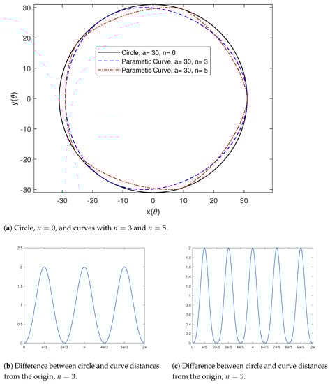
Figure 1.
Circle centered at the origin with radius a + 1 and curves with different values of n. The difference between the circle and curves; distances from the origin.
Second, we compared the ovals obtained from the parametric function (1) with different values of parameter n to a circle that is not centered at the origin, which is obtained when substituting into (1). Figure 2 shows the circle centered at with radius , which is obtained by substituting and into the parametric function (1), in comparison to curves with and , obtained by substituting and , respectively, into the same parametric function. Figure 2a shows the circle and the two curves, where we can see the vertices and the opposite points on those curves. Figure 2b shows the difference between the circle radius and the distances from the origin to any point on that curve in the case where . Similarly, Figure 2c shows the difference between the circle radius and the distances from the origin to any point on that curve in the case . Notice that in both cases, the maximum and minimum differences occur at the vertices and the opposite points, and all differences lie in the interval .
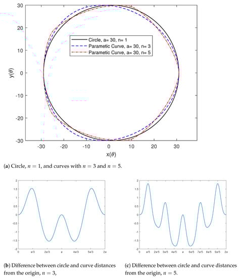
Figure 2.
Circle centered at (1,0) with radius a and curves with different values of n; the difference between circle and curves’ distances from the origin.
Finally, as a part of our simulation, we compared three ovals to two particular circles centered at the origin, which we obtained from the parametric curve in (1). The first circle has a radius of , while the second circle has a radius of . Figure 3 shows the two circles related to the three curves with , , and , obtained by substituting , , and , respectively, in the same parametric function. The choices of the parametric values for n in this simulation result and in the previous two simulation results satisfy the condition . Figure 3a shows that the three curves are bounded by the circle with the bigger radius , and for the circle with a smaller radius, . Figure 3b shows a comparison between the circles’ radii and the distances from the origin to each point on the three curves. Notice that in all three cases, the distances are enclosed in the interval , which are the radii of the two corresponding circles, which is consistent with the result from Corollary (4).
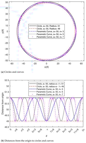
Figure 3.
Two circles centered at the origin with a = 50, and curves with different values of n, n = 3, 5, and 7.
5. Conclusions
In this study, we examined intrinsic properties of ovals of constant width, the vertices of such curves, and their lengths. For ovals of constant width with a finite number of vertices, we introduced, in addition to the new proof for Barbier’s theorem, formulas for the lengths of such curves between opposite points and between a vertex and its opposite point. We also introduced formulas for the distance between the origin and the curve points. The distance function attains its maximum and minimum values at its vertices and opposite points. The general types of ovals, discussed in the article, were compared to particular circles, and it was found that the differences in distances from the origin between the particular circles and the ovals were small and within a certain range. Finally, we showed analytically and graphically that these types of ovals are enclosed between two specific circles.
Author Contributions
Conceptualization, K.A.-B.; Methodology, A.A.-r. and K.A.-B.; Software, A.A.-r.; Validation, A.A.-r. and K.A.-B.; Formal Analysis, A.A.-r. and K.A.-B.; Investigation, A.A.-r. and K.A.-B.; Writing—Original Draft Preparation, A.A.-r. and K.A.-B.; Writing—Review and Editing, A.A.-r. and K.A.-B.; Visualization, A.A.-r. All authors have read and agreed to the published version of the manuscript.
Funding
This research received no external funding.
Data Availability Statement
All data are available from the authors upon request.
Conflicts of Interest
The authors declare no conflict of interest.
References
- Mellish, A.P. Notes on differential geometry. Ann. Math. 1931, 32, 181–190. [Google Scholar] [CrossRef]
- Al-Banawi, K. Geometry of Ovals in R2 in Terms of the Support Function. J. Appl. Sci. 2008, 8, 383–386. [Google Scholar] [CrossRef][Green Version]
- Struik, D.J. Lectures on Classical Differential Geometry; Dover Publications Inc.: New York, NY, USA, 2003. [Google Scholar]
- Al-Banawi, K.; Al-Btoush, R. Some Geometric and Analytic Properties of Closed Convex in R2. Dirasat Pure Sci. 2011, 38, 81–84. [Google Scholar]
- Resnikoff, H.L. On curves and surfaces of constant width. arXiv 2015, arXiv:1504.06733. [Google Scholar] [CrossRef]
- Fillmore, J.P. Symmetries of surfaces of constant width. J. Differ. Geom. 1969, 3, 103–110. [Google Scholar] [CrossRef]
- Al-Banawi, K.; Jaradat, O.K. A Model of the Width of an Oval via Differential Equations. World Appl. Sci. J. 2013, 23, 97–102. [Google Scholar] [CrossRef]
- Tanno, S. C∞-approximation of continuous ovals of constant width. J. Math. Soc. Jpn. 1976, 28, 384–395. [Google Scholar] [CrossRef]
- Wegner, B. Analytic approximation of continuous ovals of constant width. J. Math. Soc. Jpn. 1977, 29, 537–540. [Google Scholar] [CrossRef]
- Fu, T.; Zhou, Y. A Novel Analysis of the Smooth Curve with Constant Width Based on a Time Delay System. Mathematics 2021, 9, 1131. [Google Scholar] [CrossRef]
- Paciotti, L. Curves of constant width and their shadows. Whitman Sr. Proj. 2010, 2010, 20. [Google Scholar]
- Gibson, C.G. Elementary Geometry of Differentiable Curves: An Undergraduate Introduction; Cambridge University Press: Cambridge, UK, 2001. [Google Scholar]
- Robertson, S. Smooth curves of constant width and transnormality. Bull. Lond. Math. Soc. 1984, 16, 264–274. [Google Scholar] [CrossRef]
Disclaimer/Publisher’s Note: The statements, opinions and data contained in all publications are solely those of the individual author(s) and contributor(s) and not of MDPI and/or the editor(s). MDPI and/or the editor(s) disclaim responsibility for any injury to people or property resulting from any ideas, methods, instructions or products referred to in the content. |
© 2023 by the authors. Licensee MDPI, Basel, Switzerland. This article is an open access article distributed under the terms and conditions of the Creative Commons Attribution (CC BY) license (https://creativecommons.org/licenses/by/4.0/).