Polynomial-Time Verification of Decentralized Fault Pattern Diagnosability for Discrete-Event Systems

Abstract

This paper considers the verification of decentralized fault pattern diagnosability for discrete event systems, where the pattern is modeled as a finite automaton whose accepted language is the objective to be diagnosed. We introduce a notion of codiagnosability to formalize the decentralized fault pattern diagnosability, which requires the pattern to be detected by one of the external local observers within a bounded delay. To this end, a structure, namely a verifier, is proposed to verify the codiagnosability of the system and the fault pattern. By studying an indeterminate cycle of the verifier, sufficient and necessary conditions are provided to test the codiagnosability. It is shown that the proposed method requires polynomial time at most. In addition, we present an approach to extend the proposed verifier structure so that it can be applied to centralized cases.

1. Introduction

A discrete-event system (DES) [1,2,3] is an event-driven system whose state space is a discrete set and transitions from one state to another are triggered by the occurrence of events. The state of such a system may have logical or symbolic values that change in response to the event. In the context of DESs [2], fault diagnosis involves determining whether or not a fault has occurred with certainty [4,5]. The problem of diagnosis has been extensively studied [6,7,8,9,10]. Its formal description is located in [7]. The purpose of diagnosability is to determine whether any predetermined failure can be diagnosed within a finite delay (steps) after its occurrence. Experience with monitoring dynamic systems shows that there is a large spectrum of faulty situations in practical systems [11], such as multiple faults, intermittent faults [12], and temporary faults [13] that are not consistent with single-event faults. In order to consider these complex situations, such as temporary and/or intermittent faults, fault pattern diagnosis simultaneously emerges as a promising research area, which provides a general way to solve the diagnosis problems by capturing the occurrences of particular strings in a system and gains extensive attention from both researchers and practitioners, leading to a bulk of documented results [14,15,16,17,18,19,20].

As known, Petri nets (PNs) and finite state automata are two major tools to treat various problems in DESs. Specifically, finite state automata have been investigated for that purpose. In [14], the authors provide the ground foundations for the fault pattern diagnosis that relies on the synchronous product of a system with the pattern and the computation of the determinization of the resulting structure. Then, in [15], the same authors improve the complexity of the approach proposed in [14] by successively using the unobservable closure and a pair verifier to replace the determinization. This also introduces fault patterns in the problem of prediction. The authors of [16] address the fault pattern diagnosis by means of state isolation. In contrast to the approach in [14], which builds a diagnoser with potentially exponential complexity, the method proposed in [16] performs state estimation in a recursive manner. This approach offers the advantage of lower complexity for fault pattern detection. In [17], the authors introduce different notions of diagnosability, namely S-type and T-type pattern diagnosability, depending on whether interweaving events are accepted in the pattern. Note that this work also focuses on S-type patterns (but the T-type patterns are viewed as a particular subclass of S-type patterns, as mentioned in [17]). Moreover, in comparison to existing works, the main contribution of this paper is not only on the centralized systems but also on the decentralized frameworks, which expands the use of fault patterns.

Some contributions also consider the fault pattern diagnosis issues in PNs. On the one hand, the authors in [21] work on the diagnosability analysis of PNs by transforming the diagnosis problem into model checking. Using a particular class of PNs, the diagnosis of fault patterns has been studied according to the matching operator in [22]. With a similar approach, the same authors extended their results to the diagnosability analysis in [23]. On the other hand, stochastic PNs, endowed with Markovian semantics, have been studied to extract weak diagnosability properties for fault patterns [24]. A few researchers also consider fault patterns from the time aspects [25,26].

For the purpose of diagnosability verification, a systematic structure, namely a diagnoser, is proposed in [7], which provides the necessary and sufficient conditions for diagnosability offline. It also can be used for online fault detection based on the observations of system behaviors. The state space of a diagnoser is in the worst case exponential with respect to the size of a system model. To overcome the potential state explosion problem, a so-called “twin machine” technique [9,10], is introduced to provide a worst-case polynomial test with respect to the number of states of a system for diagnosability, without constructing a diagnoser. A state-based method for DES diagnosability is proposed in [6], which provides an algorithm for computing a sequence of test commands to detect faults.

All aforementioned works are centralized fault diagnosis, in which a centralized diagnoser is responsible for the diagnosis in a system. However, many large-sized and complex systems are physically decentralized, where diagnosis information collected by decentralized local sites will be sent to a centralized site for analysis. In this case, a variable communication delay needs to be introduced, which makes the diagnosis technique more complicated. Although all diagnosis information can be collected centrally, due to the data delay, a centralized fault diagnosis method may not always be suitable for decentralized systems.

This work focuses on the decentralized diagnosis of the DESs with multiple local observers, each of which possesses its own sensor without involving any communication among diagnosers, so as to make up for the defects of the centralized diagnosis. The authors in [27] propose a coordinated decentralized architecture with a coordinator, which extends the notion of diagnosability from centralized systems [7] to decentralized cases. In [28], a failure is characterized as a violation of a specification represented by a language, and codiagnosability is studied in a specification language framework, which is later specialized to the failure event framework. In [29], a hierarchical paradigm is developed by incorporating the protocol in [28], which leads to a hierarchy of architectures and encompasses many existing structures for decentralized diagnosis. Considering global consistency conditions, the authors in [30] discuss the diagnosis problem of the distributed setting with fault pattern and define local pattern recognizers for that purpose.

This paper deals with the decentralized fault pattern diagnosability verification of DESs, where the fault patterns are modeled by finite automata. We develop a codiagnosability notion to formalize the decentralized pattern diagnosability of the system and provide an algorithm for its verification. We first compute a synchronous product structure, which encodes a system and a pattern. A failure diagnoser structure is constructed based on the synchronous product by considering the faulty behaviors of the system, and a non-failure diagnoser is calculated based on the normal behaviors. Then, we present a local non-failure diagnoser based on the local projection. In order to verify the codiagnosability of the system and the pattern, a verifier structure is derived by taking the product of failure diagnoser and local non-failure diagnoser. By studying the indeterminate cycles of the verifier, we establish necessary and sufficient verification conditions of codiagnosability. The successive steps of the proposed approach are visualized in Figure 1.

The first contribution of the paper focuses on the construction of failure and non-failure diagnosers, which track the normal and faulty behaviors of the system, separately. The second contribution is the computation of the local diagnoser with respect to the local projection. The third contribution is to extend the necessary and sufficient conditions stated for pattern diagnosability [14] to a decentralized setting. This is achieved by constructing a verifier structure, which is the product of the failure and local non-failure diagnosers. The proposed method is shown to be of polynomial complexity. We also present a method to extend the proposed verifier so that it can be applied to centralized cases.

The rest of the paper is organized as follows. Section 2 reviews finite state automata. Section 3 begins with the notions of fault patterns and then touches upon decentralized fault pattern diagnosis in DESs. Section 4 provides an algorithm for fault pattern codiagnosability with the local diagnosers. Section 5 analyses the complexity of the proposed method. Section 6 concludes this research.

2. Preliminaries

In this paper, we use $\mathbb{N}$ to denote the set of strictly positive integers. In what follows, we consider the model of finite automaton and its related notions.

Definition 1.

A deterministic finite automaton (DFA) is a four-tuple $G=(L,\Sigma ,\delta ,l_0)$, where L is the set of states, Σ is the set of events, $l_0$ is the initial state, and $\delta :L\times \Sigma \to L$ is the partial transition function: $l^{\prime }=\delta (l,\sigma )$ means that there is a transition labeled with event $\sigma \in \Sigma$ from state l to state $l^{\prime }$. Let ${\Sigma }^{\ast }$ be the set of all finite strings defined over Σ, including the empty string λ. Transition function δ can be extended to $L\times {\Sigma }^{\ast }\to L$ in an usual way: given $l\in L$, $\mathcal{w}\in {\Sigma }^{\ast }$, and $\sigma \in \Sigma$, $\delta (l,\lambda )=l$ and $\delta (l,\mathcal{w}\sigma )=\delta \left(\right(\delta (l,\mathcal{w})),\sigma )$.

For a DFA G with partial observation, the events set $\Sigma$ can be partitioned into two disjoint subsets $\Sigma ={\Sigma }_o\cup {\Sigma }_{uo}$, where ${\Sigma }_o$ and ${\Sigma }_{uo}$ represent the set of observable events and the set of unobservable events, respectively. Given two strings ${\mathcal{w}}^{\prime },{\mathcal{w}}^{″}\in {\Sigma }^{\ast }$, the concatenation of the two strings is a string $\mathcal{w}={\mathcal{w}}^{\prime }{\mathcal{w}}^{″}\in {\Sigma }^{\ast }$, where the string ${\mathcal{w}}^{\prime }$ is followed by ${\mathcal{w}}^{″}$.

For a state $l\in L$, the set of active events at l is defined as $\Lambda \left(l\right)=\{\sigma \in \Sigma |\exists l^{\prime }\in L:l^{\prime }=\delta (l,\sigma )\}$. Given a string $\mathcal{w}\in {\Sigma }^{\ast }$, its length is defined as the number of items in $\mathcal{w}$, denoted by $\left|\mathcal{w}\right|$. A string ${\mathcal{w}}^{\prime }\in {\Sigma }^{\ast }$ is said to be a prefix of $\mathcal{w}\in {\Sigma }^{\ast }$ if there exists ${\mathcal{w}}^{″}\in {\Sigma }^{\ast }$, such that $\mathcal{w}={\mathcal{w}}^{\prime }{\mathcal{w}}^{″}$. The language generated by the DFA G is defined as $\mathcal{L}\left(G\right)=\{s\in {\Sigma }^{\ast }|\delta (l_0,s)!\}$, where $\delta (l_0,s)!$ means that “$\delta (l_0,s)$ is defined”. Given a string $\mathcal{w}\in \mathcal{L}\left(G\right)$, $\mathcal{L}\left(G\right)/\mathcal{w}$ denotes the post-language of $\mathcal{L}\left(G\right)$ after $\mathcal{w}$, defined as $\mathcal{L}\left(G\right)/\mathcal{w}=\{{\mathcal{w}}^{\prime }\in {\Sigma }^{\ast }\mid {\mathcal{ww}}^{\prime }\in \mathcal{L}\left(G\right)\}$. A run that begins with the initial state $l_0$ has the form:

$$\rho =l_0\stackrel{{\sigma }_0}{\to }{l}_1\stackrel{{\sigma }_1}{\to }\dots l_n\stackrel{{\sigma }_n}{\to }{l}_{n+1},$$

(1)

where $l_i,l_{i+1}\in L,{\sigma }_i\in \Sigma$, and $l_{i+1}=\delta (l_i,{\sigma }_i)$ for $i\in \{0,1,\dots ,n\}$. In this case, we say that the run $\rho$ is associated with the string $\mathcal{w}={\sigma }_0\dots {\sigma }_n\in {\Sigma }^{\ast }$. A run is a cycle if $l_{n+1}=l_0$.

For a decentralized system G, we use ${\Sigma }_{o_i}$ to denote the set of events observed by the local observer, simply called the local observable event set, and use ${\Sigma }_{{uo}_i}$ to denote the set of local unobservable event set, where ${\Sigma }_{{uo}_i}=\Sigma \setminus {\Sigma }_{o_i}$, $i=1,\dots ,m$, $m\in \mathbb{N}$, m is the number of the local sites. For a set of observable events ${\Sigma }_o$ of G, ${\Sigma }_o$ = ${\bigcup }_{i=1}^m{\Sigma }_{o_i}$, $i=1,\dots ,m$. Without loss of generality, we assume that there is no cycle composed only of silent events in the system G. Note that in the decentralized architecture, different sites may have events in common, i.e., for all $i,j\in \{1,\dots ,m\}$ and $i\ne j$, the set of ${\Sigma }_{o_i}\cap {\Sigma }_{o_j}$ is not necessarily an empty set. Given a site i, $i=1,\dots ,m$, the local projection ${\mathcal{P}}_i:{\Sigma }^{\ast }\to {\Sigma }_{o_i}^{\ast }$ is defined as follows: for $\mathcal{w}\in {\Sigma }^{\ast }$ and $\sigma \in \Sigma$,

$${\mathcal{P}}_i\left(\mathcal{w}\sigma \right)=\left\{\begin{array}{cc}{\mathcal{P}}_i\left(\mathcal{w}\right)\sigma \hfill & \mathrm{if}\sigma \in {\Sigma }_{o_i}\hfill \\ {\mathcal{P}}_i\left(\mathcal{w}\right)\hfill & \mathrm{otherwise},\hfill \end{array}\right.$$

(2)

and ${\mathcal{P}}_{\mathcal{i}}\left(\lambda \right)$ = $\lambda$. In other words, a local projection function ${\mathcal{P}}_i$ tracks only its corresponding local observable events. For $i=1,\dots ,m$, a site i has its own set of observable events and does not communicate with each other. For a string $\mathcal{w}$∈${\Sigma }_{o_i}^{\ast }$, the inverse of the local projection ${\mathcal{P}}_i^{-1}:2^{{\Sigma }_{o_i}^{\ast }}$ $\to 2^{{\Sigma }^{\ast }}$ is defined by ${\mathcal{P}}_i^{-1}\left(\left\{\mathcal{w}\right\}\right)$ = $\{{\mathcal{w}}^{\prime }$∈$\mathcal{L}\left(G\right)|$ ${\mathcal{P}}_i\left({\mathcal{w}}^{\prime }\right)=\mathcal{w}\}$. Let $G_1=(L_1,{\Sigma }_1,{\delta }_1,l_0^1)$ and $G_2=(L_2,{\Sigma }_2,{\delta }_2,l_0^2)$. The parallel composition is defined as $G_1\left|\right|G_2={\mathcal{P}}_1^{-1}\left(G_1\right)\times {\mathcal{P}}_2^{-1}\left(G_2\right)$, where ${\mathcal{P}}_i:{({\Sigma }_1\cup {\Sigma }_2)}^{\ast }\to {\Sigma }_i^{\ast }$, $i=1,2$.

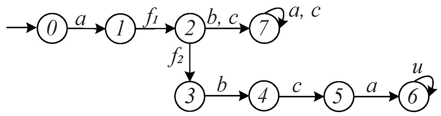
Example 1.

Consider a DFA $G_1$ shown in Figure 2 with respect to the local projection ${\mathcal{P}}_i$, $i=1,2$, where $L=\{0,1,2,3,4,5,6,7\}$ is the set of states, 0 is the initial state, $\Sigma =\{a,b,c,u,f_1,f_2\}$ is the set of events, and ${\Sigma }_o$ = $\{a,b,c\}$ is the set of observable events with ${\Sigma }_{o_1}$ = $\{a,b\}$ and ${\Sigma }_{o_2}$ = $\{a,c\}$. The transition function is defined as $\delta (0,a)$ = 1, $\delta (1,f_2)$ = 2, $\delta (2,b)$ = 7, $\delta (2,c)$ = 7, $\delta (7,a)$ = 7, $\delta (7,c)$ = 7, $\delta (2,f_2)$ = 3, $\delta (3,b)$ = 4, $\delta (4,c)$ = 5, $\delta (5,a)$ = 6, and $\delta (6,u)$ = 6. The local projection ${\mathcal{P}}_1$ of system $G_1$ is defined as ${\mathcal{P}}_1\left(a\right)$ = a, ${\mathcal{P}}_1\left(b\right)$ = b, ${\mathcal{P}}_1\left(c\right)$ = ${\mathcal{P}}_1\left(f_1\right)$ = ${\mathcal{P}}_1\left(f_2\right)$ = ${\mathcal{P}}_1\left(u\right)$ = λ, and ${\mathcal{P}}_2$ is defined as ${\mathcal{P}}_2\left(a\right)$ = a, ${\mathcal{P}}_2\left(c\right)$ = c, and ${\mathcal{P}}_2\left(b\right)$ = ${\mathcal{P}}_2\left(f_1\right)$ = ${\mathcal{P}}_2\left(f_2\right)$ = ${\mathcal{P}}_2\left(u\right)$ = λ. A possible run generated by system $G_1$ from the initial state is

$$\rho :0\stackrel{a}{\to }1\stackrel{f_1}{\to }2\stackrel{f_2}{\to }3\stackrel{b}{\to }4\stackrel{c}{\to }5\stackrel{a}{\to }6,$$

where the associated string of ρ is $\mathcal{w}=a{f}_1{f}_{2}bca$. The local projection ${\mathcal{P}}_1$ of $\mathcal{w}$ with respect to ${\Sigma }_{o_1}$ is ${\mathcal{P}}_1\left(\mathcal{w}\right)=aba$, and ${\mathcal{P}}_2$ with respect to ${\Sigma }_{o_2}$ is ${\mathcal{P}}_2\left(\mathcal{w}\right)=aca$.

3. Decentralized Fault Pattern Diagnosis of Automata

A fault pattern, simply called a pattern, is defined as a finite-state automaton whose accepted language is the objective to be diagnosed, which represents the occurrence of complex or composite faults.

Definition 2.

A (fault) pattern of a DFA $G=(L,\Sigma ,\delta ,l_0)$ is $\Omega =(S,\Sigma ,{\delta }_{\Omega },s_0,s_{\Omega })$, where S is the set of states, Σ is the set of events, $s_0\in S$ is the initial state, $s_{\Omega }\in S$ is the single final state, and ${\delta }_{\Omega }:S\times \Sigma \to S$ is the transition function. The pattern Ω satisfies a complete condition, i.e., for all $s\in S$, $\Lambda \left(s\right)=\Sigma$ and the final state $s_{\Omega }$ is stable, i.e., for all $\sigma \in \Sigma$, ${\delta }_{\Omega }(s_{\Omega },\sigma )=s_{\Omega }$.

We use ${\Sigma }_F$ to denote the set of target events that lead to the occurrence of the pattern, where ${\Sigma }_F\subseteq {\Sigma }_{uo}$. The language of pattern $\Omega$, denoted by $\mathcal{L}(\Omega )$, satisfies $\mathcal{L}(\Omega )={\Sigma }^{\ast }$ due to its complete condition. We use ${\mathcal{L}}_{\mathcal{A}}(\Omega )$ to denote the accepted language of $\Omega$, defined as ${\mathcal{L}}_{\mathcal{A}}(\Omega )=\{\mathcal{w}\in \mathcal{L}(\Omega )|{\delta }_{\Omega }(s_0,\mathcal{w})=s_{\Omega }\}$, and define the target language of DFA G as ${\mathcal{L}}_{\mathcal{A}}\left(G\right)=\mathcal{L}\left(G\right)\cap {\mathcal{L}}_{\mathcal{A}}(\Omega )$.

Example 2.

An example of pattern Ω is shown in Figure 3 with the set of states $S=\{N_1,N_2,F\}$, the set of target events ${\Sigma }_F=\{f_1,f_2\}$, the final state $s_{\Omega }=F$, and the initial state $s_0=N_1$. The accepted language of the pattern Ω is ${\mathcal{L}}_{\mathcal{A}}(\Omega )={\Sigma }^{\ast }{f}_1{\Sigma }^{\ast }{f}_2{\Sigma }^{\ast }$.

In the following, we provide a formal definition, namely codiagnosability, with respect to the decentralized system and the pattern, detailed in Definition 3.

Definition 3.

Given a DFA G, a pattern Ω, and the local projection ${\mathcal{P}}_i$, $i\in \{1,\dots ,m\}$, G is codiagnosable with regard to Ω and ${\mathcal{P}}_i$ if

$$\begin{gathered} (\exists k\in \mathbb{N}) (\forall \mathcal{w}\in {\mathcal{L}}_{\mathcal{A}}\left(G\right)) (\forall {\mathcal{w}}^{\prime }\in \mathcal{L}\left(G\right)/\mathcal{w}) \\ (\left|{\mathcal{w}}^{\prime }\right|\ge k)\Rightarrow (\exists i\in \{1,\dots ,m\})[{\mathcal{P}}_i^{-1}\left({\mathcal{P}}_i\left(\mathcal{w}{\mathcal{w}}^{\prime }\right)\right)\subseteq {\mathcal{L}}_{\mathcal{A}}\left(G\right)]. \end{gathered}$$

According to Definition 3, the system G is codiagnosable with respect to the local projection ${\mathcal{P}}_i$ and the pattern $\Omega$ if and only if for any string ${\mathcal{ww}}^{\prime }$ accepted by the pattern $\Omega$, there does not exist a string ${\mathcal{w}}^{″}$, which is not accepted by $\Omega$, such that ${\mathcal{P}}_i\left({\mathcal{ww}}^{\prime }\right)$ = ${\mathcal{P}}_i\left({\mathcal{w}}^{″}\right)$. An algorithm of fault pattern codiagnosability test is proposed based on searching for the strings ${\mathcal{ww}}^{\prime }\in {\mathcal{L}}_{\mathcal{A}}\left(G\right)$ and ${\mathcal{w}}^{″}\notin {\mathcal{L}}_{\mathcal{A}}\left(G\right)$, such that, for $i=1,\dots ,m$, the two strings ${\mathcal{ww}}^{\prime }$ and ${\mathcal{w}}^{″}$ violate the codiagnosability condition of Definition 3.

4. Verification Algorithm

For the purpose of codiagnosability verification, we propose an algorithm and a theorem in this section. Definition 4 introduces a structure that will be used later, namely synchronous product, which encodes the system G and the pattern $\Omega$.

Definition 4.

Given a DFA $G=(L,\Sigma ,\delta ,l_0)$, and a pattern $\Omega =(S,\Sigma ,{\delta }_{\Omega },s_0,s_{\Omega })$, a synchronous product $G_{\Omega }$ of G with respect to Ω is a DFA $G_{\Omega }$ = $(L_{G_{\Omega }},$ $\Sigma ,$ ${\delta }_{G_{\Omega }},$ $l_0^{G_{\Omega }},$ $L_F^{G_{\Omega }})$, where $L_{G_{\Omega }}\subseteq L\times S$ is the set of states, Σ is the set of events, $l_0^{G_{\Omega }}=(l_0,s_0)$ is the initial state, $L_F^{G_{\Omega }}=L\times \left\{s_{\Omega }\right\}$ is the set of final states, and ${\delta }_{G_{\Omega }}:(L\times S)\times \Sigma \to (L\times S)$ is the transition function, defined as follows: for $\sigma \in \Sigma$, $s,s^{\prime }\in S$, $l,l^{\prime }\in L$, ${\delta }_{G_{\Omega }}((l,s),\sigma )=(l^{\prime },s^{\prime })$ if $\delta (l,\sigma )=l^{\prime }$ and ${\delta }_{\Omega }(s,\sigma )=s^{\prime }$.

Hereafter, we propose a structure, called a verifier, which is used to test the codiagnosability of the decentralized system and the fault pattern. The successive steps of the construction are provided in Algorithm 1. Without loss of generality, we assume that $m=2$, i.e., there are two local sites with their corresponding local projections and local observable event sets.

Algorithm 1: Construction of the verifier.

Input: A pattern $\Omega$ and a DFA $G=(L,\Sigma ,\delta ,l_0)$ with two local sites, where the set of the local observable events is ${\Sigma }_{o_i}$, $i=1,2$.  Output: A verifier $G_v$ = $(L_v,\Sigma ,{\delta }_v,l_0^v)$.  1. Construct the synchronous product $G_{\Omega }$ of G and $\Omega$ according to Definition 4.  2. Compute a failure diagnoser $G_{\mathcal{f}}$ that models the faulty behaviors of the system: 1. Construct the set of states of $G_{\mathcal{f}}$ as $L_{\mathcal{f}}=\{(l,s)\in L_{G_{\Omega }}|\exists \mathcal{w}\in {\Sigma }^{*}:{\delta }_{G_{\Omega }}\left(\right(l,$ $s),\mathcal{w})\in L_F^{G_{\Omega }}\}$. 2. The initial state is $l_0^{\mathcal{f}}=l_0^{G_{\Omega }}$ if $l_0^{G_{\Omega }}$∈$L_{\mathcal{f}}$, and undefined otherwise. 3. For $l_{\mathcal{f}},l_{\mathcal{f}}^{\prime }\in L_{\mathcal{f}}$, define the transition function ${\delta }_{\mathcal{f}}:$ $L_{\mathcal{f}}$ × $\Sigma \to L_{\mathcal{f}}$ of $G_{\mathcal{f}}$ as ${\delta }_{\mathcal{f}}(l_{\mathcal{f}},$ $\sigma )=l_{\mathcal{f}}^{\prime }$ if there exists $\sigma \in \Sigma$, such that ${\delta }_{G_{\Omega }}(l_{\mathcal{f}},\sigma )=l_{\mathcal{f}}^{\prime }$. 4. Define the even set of $G_{\mathcal{f}}$ as ${\Sigma }_{\mathcal{f}}=\{\sigma \in \Sigma |$∃$l_{\mathcal{f}},$ $l_{\mathcal{f}}^{\prime }$∈$L_{\mathcal{f}}:$ ${\delta }_{\mathcal{f}}$ $(l_{\mathcal{f}},\sigma )=l_{\mathcal{f}}^{\prime }\}$. Then, $G_{\mathcal{f}}$ = $(L_{\mathcal{f}},$ ${\Sigma }_{\mathcal{f}},$ ${\delta }_{\mathcal{f}},$ $l_0^{\mathcal{f}},$ $l_F^{\mathcal{f}})$, where $L_F^{\mathcal{f}}$ is the set of final state and $L_F^{\mathcal{f}}=L_F^{G_{\Omega }}$.  3. Compute a non-failure diagnoser $G_{\mathcal{n}}$ that captures the normal behaviors of the system: 1. Construct the states set of $G_{\mathcal{n}}$ as $L_{\mathcal{n}}=\{(l,s)\in L_{G_{\Omega }}|(l,s)\in L_{G_{\Omega }}\setminus L_F^{G_{\Omega }}\}$. 2. The initial state is $l_0^{\mathcal{n}}=(l_0,s_0)$. 3. For $l_{\mathcal{n}},l_{\mathcal{n}}^{\prime }\in L_{\mathcal{n}}$, define the transition function ${\delta }_{\mathcal{n}}:L_{\mathcal{n}}\times \Sigma \to L_{\mathcal{n}}$ of $G_{\mathcal{n}}$ as ${\delta }_{\mathcal{n}}(l_{\mathcal{n}},\sigma )=l_{\mathcal{n}}^{\prime }$ if there exists $\sigma \in \Sigma$, such that ${\delta }_{G_{\Omega }}(l_{\mathcal{n}},\sigma )=l_{\mathcal{n}}^{\prime }$. 4. Define the set of events of $G_{\mathcal{n}}$ by ${\Sigma }_{\mathcal{n}}=\{\sigma \in \Sigma |$∃$l_{\mathcal{n}},$ $l_{\mathcal{n}}^{\prime }$∈$L_{\mathcal{n}}:{\delta }_{\mathcal{n}}(l_{\mathcal{n}},\sigma )=l_{\mathcal{n}}^{\prime }\}$. Then, $G_{\mathcal{n}}=(L_{\mathcal{n}},{\Sigma }_{\mathcal{n}},{\delta }_{\mathcal{n}},l_0^{\mathcal{n}})$.  4. For $i=1,2$, define function $R_i:{\Sigma }_{\mathcal{n}}\to {\Sigma }_{R_i}$ as $$R_i\left(\sigma \right)=\left\{\begin{array}{cc}\sigma \hfill & \mathrm{if}\sigma \in {\Sigma }_{o_i}\mathrm{or}\sigma \in {\Sigma }_f,\hfill \\ {\sigma }_{R_i}\hfill & \mathrm{if}\sigma \in {\Sigma }_{u{o}_i}\setminus {\Sigma }_f.\hfill \end{array}\right.$$ Construct local non-failure diagnoser $G_{{\mathcal{n}}_i}$ = $(L_{\mathcal{n}},$ ${\Sigma }_{R_i},$ ${\delta }_{{\mathcal{n}}_i},$ $l_0^{\mathcal{n}})$, where ${\delta }_{{\mathcal{n}}_i}:L_{\mathcal{n}}\times {\Sigma }_{R_i}\to L_{\mathcal{n}}$ is the transition function defined as ${\delta }_{{\mathcal{n}}_i}(l_{\mathcal{n}},R_i\left(\sigma \right))=l_{\mathcal{n}}^{\prime }$ if there exists $\sigma \in \Sigma$, $l_{\mathcal{n}},l_{\mathcal{n}}^{\prime }\in L_{\mathcal{n}}$, such that ${\delta }_{\mathcal{n}}(l_{\mathcal{n}},\sigma )=l_{\mathcal{n}}^{\prime }$.  5. Construct the verifier $G_v$ = $(L_v,$ ${\Sigma }_{R_1}\cup {\Sigma }_{R_2}\cup \Sigma ,{\delta }_v,l_0^v)$ = $G_{{\mathcal{n}}_1}\left|\right|G_{{\mathcal{n}}_2}\left|\right|G_{\mathcal{f}}$.

Note that for a state $(l_{{\mathcal{n}}_1},l_{{\mathcal{n}}_2},l_{\mathcal{f}})$ of $L_v$, it includes three components: $l_{{\mathcal{n}}_1}$, $l_{{\mathcal{n}}_2}$, and $l_{\mathcal{f}}$, where $l_{{\mathcal{n}}_1}$ is a state of $G_{{\mathcal{n}}_1}$, $l_{{\mathcal{n}}_2}$ is a state of $G_{{\mathcal{n}}_2}$, and $l_{\mathcal{f}}$ is a state of $G_{\mathcal{f}}$. The verifier $G_v$ is constructed by tracking the strings of the local non-failure diagnosers and the failure diagnoser that have the same observation with respect to the local projection ${\mathcal{P}}_i$, $i=1,2$. In other words, the transition relation ${\delta }_v$ of $G_v$ tracks three sequences: one in the local non-failure diagnoser $G_{{\mathcal{n}}_1}$, one in the local non-failure diagnoser $G_{{\mathcal{n}}_2}$, and another in the failure diagnoser $G_{\mathcal{f}}$, which generate the same sequence of observed labels.

In Step 1 of Algorithm 1, we construct a synchronous product of a system G and a pattern $\Omega$, which encodes the system and the pattern. Then, a failure diagnoser $G_{\mathcal{f}}$ is computed to track the faulty behavior of the system, which is the co-accessible part of the synchronous product with respect to the faulty strings. By Step 3, we build a non-failure diagnoser structure $G_{\mathcal{n}}$ that is the accessible part of the synchronous product by considering the normal behavior of the system. In Step 4, we establish a local non-failure diagnoser $G_{{\mathcal{n}}_i}$ based on the local projection. In this way, the event set ${\Sigma }_{u{o}_i}\setminus {\Sigma }_f$ can be renamed with respect to the local projection and the set of faulty events. Finally, by taking the product of the local non-failure diagnosers and the failure diagnoser, a verifier $G_v$ of the system G and pattern $\Omega$ can be set up, which is used to test the codiagnosability of the decentralized system.

Definition 5.

Given the verifier $G_v$ of a DFA G and a pattern Ω, for $0<m\le n$, m, $n\in \mathbb{N}$, a cycle $cl:$ $l_v^m,$ ${\sigma }_m,$ $l_v^{m+1},$ $\dots ,l_v^n,{\sigma }_n,l_v^m$ of $G_v$ is said to be an indeterminate cycle if for state $l_v^j=(l_{{\mathcal{n}}_1}^j,l_{{\mathcal{n}}_2}^j,l_{\mathcal{f}}^j)\in L_v$, $j=m,m+1,\dots ,n$, $l_{\mathcal{f}}^j\in L_F^{\mathcal{f}}$, and there exists ${\sigma }_j$, $j\in \{m,m+1,\dots ,n\}$, such that ${\sigma }_j\in \Sigma$.

Theorem 1.

Let G be a DFA with the local projection ${\mathcal{P}}_i$, $i=1,2$, and a pattern Ω. G is not codiagnosable with respect to ${\mathcal{P}}_i$ and Ω if and only if there exists an indeterminate cycle in $G_v$.

Proof. 

(if) Suppose that there exists an indeterminate cycle $cl:$ $l_v^m,{\sigma }_m,l_v^{m+1},\dots ,l_v^n,{\sigma }_n,l_v^m$. Then, there exists a string $s_v{t}_v$ generating a run $l_0^v,{\sigma }_0,\dots ,l_v^m,{\sigma }_m,l_v^{m+1},\dots ,l_v^n,{\sigma }_n,l_v^m$ in $G_v$, such that for $j=m,m+1,\dots ,n$, $l_{\mathcal{f}}^j\in L_F^{\mathcal{f}}$. Define

$${\mathcal{P}}_{R_1}:{({\Sigma }_{R_1}\cup {\Sigma }_{R_2}\cup \Sigma )}^{\ast }\to {\Sigma }_{R_1}^{\ast },$$

(3)

$${\mathcal{P}}_{R_2}:{({\Sigma }_{R_1}\cup {\Sigma }_{R_2}\cup \Sigma )}^{\ast }\to {\Sigma }_{R_2}^{\ast },$$

(4)

$${\mathcal{P}}_{\Sigma }:{({\Sigma }_{R_1}\cup {\Sigma }_{R_2}\cup \Sigma )}^{\ast }\to {\Sigma }^{\ast }.$$

(5)

By $G_v$ = $G_{{\mathcal{n}}_1}\left|\right|G_{{\mathcal{n}}_2}\left|\right|G_{\mathcal{f}}$, it concludes that $\mathcal{L}\left(G_v\right)={\mathcal{P}}_{R_1}^{-1}\left(\mathcal{L}\left(G_{{\mathcal{n}}_1}\right)\right)$∩${\mathcal{P}}_{R_2}^{-1}\left(\mathcal{L}\left(G_{{\mathcal{n}}_2}\right)\right)$∩${\mathcal{P}}_{\Sigma }^{-1}\left(\mathcal{L}\left(G_{\mathcal{f}}\right)\right)$, where $\mathcal{L}\left(G_v\right)$, $\mathcal{L}\left(G_{{\mathcal{n}}_i}\right)$, and $\mathcal{L}\left(G_{\mathcal{f}}\right)$ are the generated languages of $G_v$, $G_{{\mathcal{n}}_i}$, $i=1,2$, and $G_{\mathcal{f}}$, respectively. Consequently, there exists a string $st={\mathcal{P}}_{\Sigma }\left(s_v{t}_v\right)$ in $G_{\mathcal{f}}$, such that $s={\mathcal{P}}_{\Sigma }\left(s_v\right)\in {\mathcal{L}}_{\mathcal{A}}\left(G\right)$, $t={\mathcal{P}}_{\Sigma }\left(t_v\right)$, and $st\in {\mathcal{L}}_{\mathcal{A}}\left(G\right)$ (see Step 2 of Algorithm 1).

Let $s_{R_1}={\mathcal{P}}_{R_1}\left(s_v{t}_v\right)$. There exists a string $s_1$ in $G_{\mathcal{n}}$, such that ${\mathcal{P}}_{\Sigma }\left(s_{R_1}\right)=s_1$ and ${\mathcal{P}}_{\Sigma }\left(s_{R_1}\right)={\mathcal{P}}_{\Sigma }\left({\mathcal{P}}_{R_1}\left(s_v{t}_v\right)\right)$. With a slight abuse of notation, we have ${\mathcal{P}}_1\left(s_1\right)={\mathcal{P}}_1\left(st\right)$. Similar to $s_{R_1}$, there exists a string $s_{R_2}$ in $G_{{\mathcal{n}}_2}$ and $s_2$ in $G_{\mathcal{n}}$, such that $s_2={\mathcal{P}}_{\Sigma }\left(s_{R_2}\right)$. For the same reason, we have ${\mathcal{P}}_2\left(s_2\right)={\mathcal{P}}_2\left(st\right)$, where $st\in {\mathcal{L}}_{\mathcal{A}}\left(G\right)$, and $s_1,s_2\notin {\mathcal{L}}_{\mathcal{A}}\left(G\right)$ (see Step 3 of Algorithm 1). For the string $s_v{t}_v$ with arbitrary length, the strings $s_1$ and $s_2$ can also be extended long enough. This implies that G is not codiagnosable with respect to pattern $\Omega$ and local projection ${\mathcal{P}}_i$.

(only if) Suppose that G is not codiagnosable with respect to $\Omega$ and ${\mathcal{P}}_i$. Then, there exists a string $s\in {\mathcal{L}}_{\mathcal{A}}\left(G\right)$, $t\in {\mathcal{L}}_{\mathcal{A}}\left(G\right)/s$, and strings $s_1,s_2\notin {\mathcal{L}}_{\mathcal{A}}\left(G\right)$, such that ${\mathcal{P}}_1\left(s_1\right)={\mathcal{P}}_1\left(st\right)$, ${\mathcal{P}}_2\left(s_2\right)={\mathcal{P}}_2\left(st\right)$.

According to Steps 3 and 4 of Algorithm 1, there exists a string $s_{R_1}$ in $G_{{\mathcal{n}}_1}$ and a string $s_{R_2}$ in $G_{{\mathcal{n}}_2}$, such that $s_{R_1}$ = $R_1\left(s_1\right)$ and $s_{R_2}$ = $R_1\left(s_2\right)$, where R can be extended from $\Sigma$ to ${\Sigma }^{\ast }$ as the usual way. Consider two prefixes $s_{R_1}^{\prime }$ of $s_{R_1}$ and $s_{R_2}^{\prime }$ of $s_{R_2}$, such that ${\mathcal{P}}_1\left({\mathcal{P}}_{\Sigma }\left(s_{R_1}^{\prime }\right)\right)={\mathcal{P}}_1\left(s\right)$ and ${\mathcal{P}}_2\left({\mathcal{P}}_{\Sigma }\left(s_{R_2}^{\prime }\right)\right)={\mathcal{P}}_2\left(s\right)$. Since $s_1,s_2\notin {\mathcal{L}}_{\mathcal{A}}\left(G\right)$, ${\mathcal{P}}_{\Sigma }\left(s_{R_1}^{\prime }\right),{\mathcal{P}}_{\Sigma }\left(s_{R_2}^{\prime }\right)\notin {\mathcal{L}}_{\mathcal{A}}\left(G\right)$ holds. As a result, there exist two runs in $G_{{\mathcal{n}}_1}$ and $G_{{\mathcal{n}}_2}$, beginning from $l_0^{\mathcal{n}}$ and generated by $s_{R_1}^{\prime }$, $s_{R_2}^{\prime }$, respectively, with the forms

$${\rho }_{s_{R_1}^{\prime }}:l_0^{\mathcal{n}}\stackrel{s_{R_1}^{\prime }}{\to }{l}_{s_{R_1}^{\prime }},\mathrm{and}{\rho }_{s_{R_2}^{\prime }}:l_0^{\mathcal{n}}\stackrel{s_{R_2}^{\prime }}{\to }{l}_{s_{R_2}^{\prime }}.$$

(6)

In addition, since $s\in {\mathcal{L}}_{\mathcal{A}}\left(G\right),$ according to Step 2 of Algorithm 1, there exists a run in $G_{\mathcal{f}}$ beginning from $l_0^{\mathcal{f}}$ generated by s with the form of ${\rho }_s:l_0^{\mathcal{f}}\stackrel{s}{\to }{l}_s$.

Similarly, three runs in $G_{{\mathcal{n}}_1}$, $G_{{\mathcal{n}}_2}$, $G_{\mathcal{f}}$ can be generated by $s_{R_1}$, $s_{R_2}$, $st$, respectively, with the form of

$${\rho }_{s_{R_1}}:l_0^{\mathcal{n}}\stackrel{s_{R_1}}{\to }{l}_{s_{R_1}},{\rho }_{s_{R_2}}:l_0^{\mathcal{n}}\stackrel{s_{R_2}}{\to }{l}_{s_{R_2}},\mathrm{and}{\rho }_{st}:l_0^{\mathcal{f}}\stackrel{st}{\to }{l}_{st}$$

(7)

such that ${\mathcal{P}}_1\left({\mathcal{P}}_{\Sigma }\left(s_{R_1}\right)\right)={\mathcal{P}}_1\left(st\right)$ and ${\mathcal{P}}_2\left({\mathcal{P}}_{\Sigma }\left(s_{R_2}\right)\right)={\mathcal{P}}_1\left(st\right)$. Then, there exists a run in $G_v$ of the form

$${\rho }_v:l_0^v\to \dots \to l_v^m\to \dots \to l_v^n$$

(8)

such that $l_v^m=(l_{s_{R_1}^{\prime }},l_{s_{R_2}^{\prime }},l_s)$ and $l_v^m=(l_{s_{R_1}},l_{s_{R_2}},l_{st})$.

The strings $s_{R_1}$ and $s_{R_1}$ are extended from the string $st$ to be as large as possible. Then, there eventually exist two states $l_v^i$, $l_v^j$ in ${\rho }_v$, $m\le i\le j\le n$, such that $l_v^i=l_v^j$. For $r=i,i+1,\dots ,j$, the set of states $\left\{l_v^r\right\}$ of $G_V$ form an indeterminate cycle. This contradicts the assumption and ends the proof. □

Theorem 1 provides an approach to verify codiagnosability by searching for the existence of indeterminate cycles. In the case of at least one indeterminate cycle, there are at least three strings $s_1$, $s_2$, and $s_3$ with arbitrary length in non-failure diagnosers $G_{{\mathcal{n}}_1}$, $G_{{\mathcal{n}}_2}$, and the failure diagnoser $G_{\mathcal{f}}$, respectively, where $s_1$ and $s_3$ have the same observation with respect to the projection ${\mathcal{P}}_1$, and $s_2$ and $s_3$ have the same observation with respect to the projection ${\mathcal{P}}_2$, violating the codiagnosability.

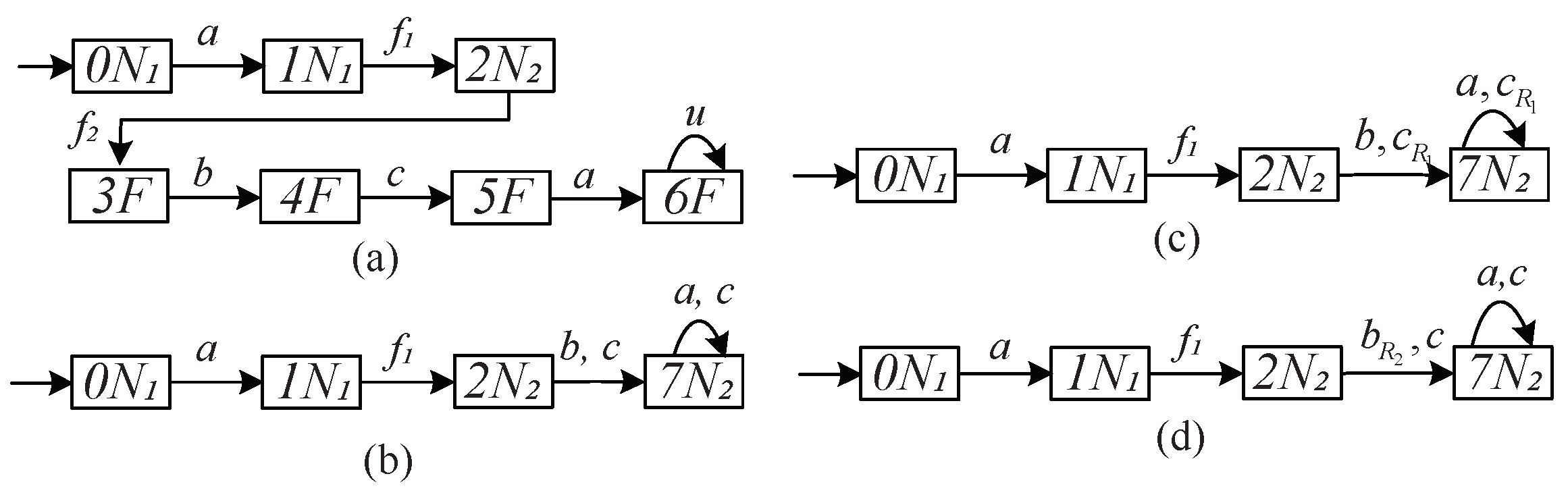
Example 3.

Consider a DFA $G_1$ shown in Figure 2 with the local observable event set ${\Sigma }_{o_i}$, $i=1,2$, and a pattern Ω shown in Figure 3. According to the first step of Algorithm 1, we construct the synchronous product $G_{1\Omega }$, as shown in Figure 4, which encodes the information of the system $G_1$ and the fault pattern Ω. The second step is to obtain the failure diagnoser $G_{1\mathcal{f}}$, which is the co-accessible part of $G_{1\Omega }$ with respect to the set of the faulty states $L_F^{G_{1\Omega }}$, as shown in Figure 5a. It should be noted that all accepted behaviors of the failure diagnoser $G_{1\mathcal{f}}$ are faulty behaviors. Continuing Algorithm 1, we compute a non-failure diagnoser $G_{1\mathcal{n}}$ by taking the accessible part of $G_{1\Omega }$ regarding the set of normal states $L_{G_{1\Omega }}\setminus L_F^{G_{1\Omega }}$, as shown in Figure 5b. Note that all generated behaviors of the non-failure diagnoser $G_{1\mathcal{n}}$ are normal behaviors. Based on Step 4, we can calculate the local non-failure diagnosers $G_{1{\mathcal{n}}_1}$ and $G_{1{\mathcal{n}}_2}$, respectively, by renaming the unobservable event sets ${\Sigma }_{{uo}_1}\setminus {\Sigma }_f=\left\{c\right\}$ and ${\Sigma }_{{uo}_2}\setminus {\Sigma }_f=\left\{b\right\}$ based on function $R_i$, as shown in Figure 5c,d. It shows that the sets of the events of the local non-failure diagnosers $G_{1{\mathcal{n}}_1}$ and $G_{1{\mathcal{n}}_2}$ are ${\Sigma }_{R_1}=\{a,b,f_1,c_{R_1}\}$ and ${\Sigma }_{R_2}=\{a,b_{R_2},f_1,c\}$, respectively. The final step of Algorithm 1 is the computation of the verifier $G_{1v}$ of $G_1$ and Ω, which is obtained by $G_{1v}=$ $G_{{1\mathcal{n}}_1}\left|\right|G_{{1\mathcal{n}}_2}\left|\right|G_{\mathcal{f}}$, as shown in Figure 6.

According to Theorem 1, one can know that the verification of the fault pattern codiagnosability is to search for the indeterminate cycles in $G_{1v}$. The verifier of Figure 6 has several cycles (for example, the cycles $7N_{2}7N_{2}2N_2\stackrel{C_{R_1}}{\to }7N_{2}7N_{2}2N_2$, $7N_{2}7N_{2}6F\stackrel{C_{R_1}}{\to }7N_{2}7N_{2}6F$, and $7N_{2}7N_{2}6F\stackrel{u}{\to }7N_{2}7N_{2}6F$). Notice that only the cycle $7N_{2}7N_{2}6F\stackrel{u}{\to }7N_{2}7N_{2}6F$ is an indeterminate cycle (Definition 5). The existence of the indeterminate cycle $7N_{2}7N_{2}6F\stackrel{u}{\to }7N_{2}7N_{2}6F$ implies that the system $G_1$ is not codiagnosable with respect to the local projection ${\mathcal{P}}_i$, $i=1,2$, and the pattern Ω (Theorem 1).

Example 4.

Consider a DFA $G_2$ shown in Figure 7a with the local projection ${\mathcal{P}}_i$, $i=1,2$ and a pattern Ω in Figure 3, where $\Sigma =\{a,b,c,f_1,f_2\}$ is the set of events, ${\Sigma }_{o_1}$ = $\{a,b\}$, and ${\Sigma }_{o_2}$ = $\{a,c\}$. According to the first step of Algorithm 1, we can construct the synchronous product $G_{2\Omega }$, as shown in Figure 7b. Continuing Algorithm 1, the failure diagnoser $G_{2\mathcal{f}}$ can be computed accordingly, as shown in Figure 8a. By Steps 3 and 4 of Algorithm 1, we can obtain the non-failure diagnosers and the local non-failure diagnosers successively. For the sake of simplicity, we keep the local non-failure diagnosers $G_{2{\mathcal{n}}_1}$ and $G_{1{\mathcal{n}}_2}$, which will be used later, as shown in Figure 8b,c. Continuing Step 5 of Algorithm 1, we can calculate the verifier $G_{2v}$ with respect to the local projections, as shown in Figure 8d.

Observe that there exist three cycles in the verifier $G_{2v}$, i.e., $5N_{2}2N_{2}4F\stackrel{C_{R_1}}{\to }5N_{2}2N_{2}4F$, $5N_{2}5N_{2}4F\stackrel{C_{R_1}}{\to }5N_{2}5N_{2}4F$, and $5N_{2}5N_{2}4F\stackrel{C}{\to }5N_{2}5N_{2}4F$, and the cycle $5N_{2}5N_{2}4F\stackrel{C}{\to }5N_{2}5N_{2}4F$ is indeterminate (Definition 5). As a consequence, the system $G_2$ is not codiagnosable with respect to the local projection ${\mathcal{P}}_i$, $i=1,2$, and the pattern Ω (Theorem 1).

Example 5.

In order to compare the codiagnosability with the system $G_2$, we consider a DFA $G_3$, as shown in Figure 9a, and the pattern Ω in Figure 3. The local projection of $G_3$ is ${\mathcal{P}}_i$, $i=1,2$, where $\Sigma =\{a,b,c,d,f_1,f_2\}$ is the set of events, ${\Sigma }_{o_1}$ = $\{a,b,d\}$, and ${\Sigma }_{o_2}$ = $\{a,$ $c,d\}$. Following Algorithm 1, the resulting structure can be obtained step by step. For simplicity, we detail the verifier $G_{3v}$, as shown in Figure 9b. Note that there is no indeterminate cycle (Definition 5). This implies that the system $G_3$ is codiagnosable with respect to the local projection and the pattern Ω (Theorem 1).

Note that the pattern diagnosability verification in the centralized case can be easily obtained by marking $m=1$ of Algorithm 1, i.e., the number of the local site is 1. Therefore, the verifier automaton for the centralized case is given as $G_{v_c}=G_{{\mathcal{n}}_1}\left|\right|G_{\mathcal{f}}$, and the necessary and sufficient condition for the non-diagnosability of G is the existence of an indeterminate cycle in $G_{v_c}$, such that at least one event in the cycle is an event of $\Sigma$.

5. Complexity Analysis

From Definitions 1 and 2, we know that the number of states of the system G is $\left|L\right|$, and the number of states of the pattern $\Omega$ is $\left|S\right|$. Assume that the number of the local sites is m.

The complexity of performing Step 1 of Algorithm 1, which constructs the synchronous product $G_{\Omega }$, is $O\left(\right|L|\times |S\left|\right)$, and that of Step 2 of Algorithm 1, which constructs the failure diagnoser $G_{\mathcal{f}}$, is $O\left(\right|L|\times |S\left|\right)$. The complexity of performing Step 3 of Algorithm 1, which computes the non-failure diagnoser $G_{\mathcal{n}}$ by deleting all the final states of $G_{\Omega }$, is $O\left(\right|L|\times |S\setminus \left\{s_{\Omega }\right\}\left|\right)$. The complexity of obtaining the local non-failure diagnoser $G_{{\mathcal{n}}_i}$ in Step 4 of Algorithm 1, $i=1,\dots ,m$, is $O\left(\right|L|\times |S\setminus \left\{s_{\Omega }\right\}\left|\right)$. By Step 5, the complexity of verifier $G_v$ construction is $O\left(\right|L{|}^m\times |S\setminus \left\{s_{\Omega }\right\}{|}^m\times |L|\times |S\left|\right)$.

Thus, the complexity of Algorithm 1 is $O\left(\right|L{|}^{m+1}\times |S\setminus \left\{s_{\Omega }\right\}{|}^m\times |S\left|\right)$, which is polynomial with respect to the number of the states of G and $\Omega$, i.e., $O\left({\left(\right|L\left|\right|S\left|\right)}^{m+1}\right)$.

6. Conclusions

The objective of this work is the verification of pattern diagnosability for decentralized DESs. In particular, the fault patterns are modeled by finite automata, providing a general way to formalize different types of failures. This improves the method in [29,31], which only targets single fault scenarios. To this end, we introduce a codiagnosability notion to encapsulate decentralized fault pattern diagnosability, and present an algorithm to test this property. In detail, we first compute a synchronous product structure to encode the system and the pattern. A failure diagnoser and a non-failure diagnoser are calculated based on the synchronous product, where the two structures are obtained by considering the normal and faulty behaviors, respectively. Then, we present a local non-failure diagnoser based on the local projection of the system. A verifier for codiagnosability verification is derived by taking the product of the failure diagnoser with the local non-failure diagnoser. Consequently, the verifier structure can track the strings of the failure and local non-failure diagnosers that have the same observations. The proposed method boasts polynomial complexity, marking an improvement over methods in [17,21]. Moreover, the approach proposed in this paper can be used for decentralized systems as well as centralized systems, enhancing the method presented in [14,15] for centralized systems.

Our future work will consider decentralized diagnosis issues of timed fault patterns, which are characterized by a sequence of events that occur in a given order at specific values of time or within specific time intervals. In certain cases, the time value of the system is compulsory. For example, in some flexible manufacturing systems, the operation of the robot must be finished in a specified time. At this point, a time value needs to be assigned to each event of the system, and the diagnoser should be calculated based on not only the event but also the time value. Another limitation of the algorithm is that an external attack is not considered in the system. With this in mind, we will consider different types of attack forms in future work, including insertion, deletion, and replacement of observations. These observations refer to sequences of observable events observed by external observers as well as intruders (aliases of attackers). Such tampering with system-generated observations may mislead system operators to make inexact, conservative, or even incorrect state estimations that are critical for many problems in the context of DESs, such as supervisory control, opacity verification, enforcement, detectability analysis, and fault diagnosis. Certainly, these problems can be addressed under the framework of centralized and/or decentralized system architectures.