Stability of the Exponential Type System of Stochastic Difference Equations

Abstract

The method of studying the stability in the probability for nonlinear systems of stochastic difference equations is demonstrated on two systems with exponential and fractional nonlinearities. The proposed method can be applied to nonlinear systems of higher dimensions and with other types of nonlinearity, both for difference equations and for differential equations with delay.

1. Introduction

Nonlinear differential and difference equations, particularly equations with exponential nonlinearity, are very popular in research (see, for instance, [1,2,3,4,5,6,7,8,9,10,11,12,13]) and have numerous applications, such as Nicholson’s blowflies equation, mosquito population equations, the neoclassical growth model (see, for instance, [2,10,12,13] and the references therein).

The importance of studying difference equations both for theory and for numerous applications is particularly shown in monographs [14,15,16,17,18], where nonlinear and, in particular, rational difference equations are especially highlighted.

Here, the system of three difference equations with exponential nonlinearity

$$\begin{array}{c}{x}_1(n+1)=a_1{x}_1\left(n\right)+(b_1{x}_2(n-1)+c_1{x}_3(n-1))e^{-{\mu }_1{x}_1\left(n\right)},\\ x_2(n+1)=a_2{x}_2\left(n\right)+(b_2{x}_3(n-1)+c_2{x}_1(n-1))e^{-{\mu }_2{x}_2\left(n\right)},\\ x_3(n+1)=a_3{x}_3\left(n\right)+(b_3{x}_1(n-1)+c_3{x}_2(n-1))e^{-{\mu }_3{x}_3\left(n\right)},\\ n\in N=\{0,1,\dots \},\end{array}$$

(1)

and the initial conditions

$$x_1\left(j\right)={\phi }_1\left(j\right),x_2\left(j\right)={\phi }_2\left(j\right),x_3\left(j\right)={\phi }_3\left(j\right),j\in N_0=\{-1,0\},$$

are considered. It was assumed that all the parameters of system (1) were positive and that

$$a_i<1,i=1,2,3.$$

(2)

It is shown that system (1) has both zero and nonzero (positive or negative) equilibria. The stability of all types of equilibria of system (1) was investigated under stochastic perturbations via the general method of Lyapunov functional construction [12,13] and the method of linear matrix inequalities (LMIs) [19,20,21,22,23,24,25,26,27]. Numerical analysis of the considered LMIs was carried out using MATLAB.

The method of studying stability used here is of a fairly general nature and can be applied to nonlinear systems that are described by both difference and differentials equations [28,29,30]. To demonstrate that this method can be used for systems of higher dimension and for systems with other types of nonlinearity, besides of system (1), a special system with exponential and fractional nonlinearities was also investigated.

Further in the paper, the necessary definitions and theorems of stability are given, the calculations and investigations of the equilibria are presented, the problem of stability under stochastic perturbations is formulated, the obtained results are illustrated by numerical simulation, by the figures and by work with a special program from the MATLAB.

Such detailed descriptions of the required steps of research will allow potential readers to apply the proposed method to the study of other nonlinear systems in various applications. An unsolved problem is also brought to the attention of readers, the solution of which may give the method under consideration some additional interesting possibilities.

2. Equilibria

The equilibria $E^{*}(x_1,x_2,x_3)$ of system (1) are defined by the system of the following three algebraic equations:

$$\begin{array}{c}(1-a_1)x_1=(b_1{x}_2+c_1{x}_3)e^{-{\mu }_1{x}_1},\\ (1-a_2)x_2=(b_2{x}_3+c_2{x}_1)e^{-{\mu }_2{x}_2},\\ (1-a_3)x_3=(b_3{x}_1+c_3{x}_2)e^{-{\mu }_3{x}_3}.\end{array}$$

(3)

It is obvious that system (3) has the zero solution; therefore, the system under consideration (1) has the zero equilibrium $E_0^{*}(0,0,0)$.

Through putting in (3) $x_1=x_2=x_3=x$, we determine that, for arbitrary $x\ne 0$, system (1) can have an equilibrium $E^{*}(x,x,x)$ with the same coordinates. By this, from (3), we obtain

$$e^{{\mu }_{i}x}=\frac{b_i+c_i}{1-a_i},{\mu }_i=\frac{1}{x}ln\left(\frac{b_i+c_i}{1-a_i}\right),i=1,2,3.$$

(4)

Remark 1.

In the case of (4), due to the positiveness of the parameters ${\mu }_i$, $i=1,2,3$, the following two situations are possible: (1) $a_i+b_i+c_i>1$ and $x>0$, (2) $a_i+b_i+c_i<1$ and $x<0$.

Note that system (1) cannot have an equilibrium with one or two zero coordinates. Thus, putting in (3), for instance, $x_1=0$, we obtain the following:

$$\begin{array}{c}{b}_1{x}_2+c_1{x}_3=0,\hfill \\ (1-a_2)x_2=b_2{x}_3{e}^{-{\mu }_2{x}_2},\hfill \\ (1-a_3)x_3=c_3{x}_2{e}^{-{\mu }_3{x}_3}.\hfill \end{array}$$

(5)

From the first equation of (5), it follows that $x_2$ and $x_3$ must have different signs; however, via two other equations, it is clear that this is impossible. Assuming that some two coordinates are zero, from (3), we obtain that the third coordinate is also zero.

Arguing similarly, it is easy to understand that all coordinates of a non-zero equilibrium must be of the same sign. So, system (1) has the zero equilibrium $E_0^{*}(0,0,0)$ and can have some equilibria $E^{*}(x_1,x_2,x_3)$ with all nonzero (all positive or all negative) coordinates.

Let us consider conditions for existence of a positive equilibrium.

Lemma 1.

If system (1) has an equilibrium $E_{+}^{*}(x_1,x_2,x_3)$ with $x_i>0$, $i=1,2,3$, then it satisfies the conditions

$${\alpha }_1<{\mu }_2{x}_2+{\mu }_3{x}_3,{\alpha }_2<{\mu }_1{x}_1+{\mu }_3{x}_3,{\alpha }_3<{\mu }_1{x}_1+{\mu }_2{x}_2,$$

(6)

where

$${\alpha }_1=ln\frac{b_2{c}_3}{(1-a_2)(1-a_3)},{\alpha }_2=ln\frac{b_3{c}_1}{(1-a_1)(1-a_3)},{\alpha }_3=ln\frac{b_1{c}_2}{(1-a_1)(1-a_2)}.$$

(7)

Proof. 

Let $(x_1,x_2,x_3)$ be a solution of system (3) with $x_i>0$, $i=1,2,3$. Then, from the last two equations of system (3), we obtain

$$\begin{array}{cc}{x}_1& =\frac{1}{c_2}[(1-a_2)x_2{e}^{{\mu }_2{x}_2}-b_2{x}_3]>0,\\ x_1& =\frac{1}{b_3}[(1-a_3)x_3{e}^{{\mu }_3{x}_3}-c_3{x}_2]>0.\end{array}$$

Using $(1-a_2)x_2{e}^{{\mu }_2{x}_2}>b_2{x}_3$, $(1-a_3)x_3{e}^{{\mu }_3{x}_3}>c_3{x}_2$, and (2), we obtain

$$\frac{c_3{e}^{-{\mu }_3{x}_3}}{1-a_3}<\frac{x_3}{x_2}<\frac{(1-a_2)e^{{\mu }_2{x}_2}}{b_2},$$

from which the condition (6) for ${\alpha }_1$ follows.

Similarly, from the first and the last equations of system (3), and from the first two equations of system (3), we, respectively, obtain

$$\begin{array}{cc}{x}_2& =\frac{1}{c_3}[(1-a_3)x_3{e}^{{\mu }_3{x}_3}-b_3{x}_1]>0,\\ x_2& =\frac{1}{b_1}[(1-a_1)x_1{e}^{{\mu }_1{x}_1}-c_1{x}_3]>0,\end{array}$$

and

$$\begin{array}{cc}{x}_3& =\frac{1}{c_1}[(1-a_1)x_1{e}^{{\mu }_1{x}_1}-b_1{x}_2]>0,\\ x_3& =\frac{1}{b_2}[(1-a_2)x_2{e}^{{\mu }_2{x}_2}-c_2{x}_1]>0.\end{array}$$

Therefore,

$$\frac{c_1{e}^{-{\mu }_1{x}_1}}{1-a_1}<\frac{x_1}{x_3}<\frac{(1-a_3)e^{{\mu }_3{x}_3}}{b_3}$$

and

$$\frac{c_2{e}^{-{\mu }_2{x}_2}}{1-a_2}<\frac{x_2}{x_1}<\frac{(1-a_1)e^{{\mu }_1{x}_1}}{b_1},$$

from which the conditions (6) for ${\alpha }_2$ and ${\alpha }_3$ follow. Thus, the proof is completed. □

Corollary 1.

If system (1) has an equilibrium $E_{-}^{*}(x_1,x_2,x_3)$ with $x_i<0$, $i=1,2,3$, then it satisfies the conditions

$${\alpha }_1<{\mu }_2{x}_2+{\mu }_3{x}_3<0,{\alpha }_2<{\mu }_1{x}_1+{\mu }_3{x}_3<0,{\alpha }_3<{\mu }_1{x}_1+{\mu }_2{x}_2<0,$$

(8)

where ${\alpha }_i$ are given in (7).

Proof is the same as in Lemma 1.

Lemma 2.

Let the following conditions hold

$$\begin{array}{c}{b}_2{c}_3\ge (1-a_2)(1-a_3),\\ b_3{c}_1\ge (1-a_1)(1-a_3),\\ b_1{c}_2\ge (1-a_1)(1-a_2).\end{array}$$

(9)

Then, system (1) has an equilibrium $E_{+}^{*}(x_1,x_2,x_3)$ with $x_i>0$, $i=1,2,3$.

Proof. 

Let us show that, by the conditions (9), system (3) has the solution $(x_1,x_2,x_3)$ with $x_i>0$, $i=1,2,3$. From (7), it follows that the conditions (9) are equivalent to the conditions ${\alpha }_i\ge 0$, $i=1,2,3$. Therefore, via (6), no pair of coordinates from $x_1$, $x_2$, $x_3$ can be non-positive. But, from (3), it follows that if any two coordinates from $x_1$, $x_2$, $x_3$ are positive then the third coordinate is also positive. Thus, the proof is completed. □

3. Stochastic Perturbations, Centralization and Linearization

Let $\{\Omega ,\mathfrak{F},\mathbf{P}\}$ be a basic probability space, ${\mathfrak{F}}_n\subset \mathfrak{F}$, $n\in N$, a nondecreasing family of sub-$\sigma$-algebras of $\mathfrak{F}$, i.e., ${\mathfrak{F}}_{n_1}\subset {\mathfrak{F}}_{n_2}$ for $n_1<n_2$; $\mathbf{E}$ be the mathematical expectation with respect to the measure $\mathbf{P}$; ${\xi }_i\left(n\right)$, $i=1,2,3$, $n\in N$, be three mutually independent sequences with ${\mathfrak{F}}_n$-adapted mutually independent random values such that [12]

$$\mathbf{E}{\xi }_i\left(n\right)=0,\mathbf{E}{\xi }_i^2\left(n\right)=1,\mathbf{E}{\xi }_i\left(n\right){\xi }_j\left(m\right)=0\mathrm{if}i\ne j\mathrm{or}n\ne m.$$

(10)

Let $E^{*}(x_1^{*},x_2^{*},x_3^{*})$ be one of the possible equilibria of system (1), including the zero equilibrium. Let us suppose that system (1) is exposed to stochastic perturbations that are directly proportional to the deviation of the system state $(x_1\left(n\right),x_2\left(n\right),x_3\left(n\right))$ from the equilibrium $E^{*}(x_1^{*},x_2^{*},x_3^{*})$, i.e., system (1) takes the form of the system of stochastic difference equations [12]:

$$\begin{array}{c}{x}_1(n+1)=a_1{x}_1\left(n\right)+(b_1{x}_2(n-1)+c_1{x}_3(n-1))e^{-{\mu }_1{x}_1\left(n\right)}+{\sigma }_1(x_1\left(n\right)-x_1^{*}){\xi }_1(n+1),\\ x_2(n+1)=a_2{x}_2\left(n\right)+(b_2{x}_3(n-1)+c_2{x}_1(n-1))e^{-{\mu }_2{x}_2\left(n\right)}+{\sigma }_2(x_2\left(n\right)-x_2^{*}){\xi }_2(n+1),\\ x_3(n+1)=a_3{x}_3\left(n\right)+(b_3{x}_1(n-1)+c_3{x}_2(n-1))e^{-{\mu }_3{x}_3\left(n\right)}+{\sigma }_3(x_3\left(n\right)-x_3^{*}){\xi }_3(n+1),\end{array}$$

(11)

where ${\sigma }_i$, $i=1,2,3$, is some number that is called a level of noise.

Note that the equilibrium $E^{*}(x_1^{*},x_2^{*},x_3^{*})$ of the deterministic system (1) is also the solution of the stochastic system (11). Stochastic perturbations of such a type were first proposed in [31], and they were successfully used later by many other researchers for different mathematical models with continuous and discrete time applications (see, for instance, [10,11,12,13,28,29,30] and the references therein).

By substituting into system (11) $x_i\left(n\right)=y_i\left(n\right)+x_i^{*}$, $i=1,2,3$, and using (3), we centralize system (11) around the equilibrium $E^{*}(x_1^{*},x_2^{*},x_3^{*})$

$$\begin{array}{c}{y}_1(n+1)=a_1{y}_1\left(n\right)+[b_1{y}_2(n-1)+c_1{y}_3(n-1)]e^{-{\mu }_1(y_1\left(n\right)+x_1^{*})}\\ +(1-a_1)x_1^{*}(e^{-{\mu }_1{y}_1\left(n\right)}-1)+{\sigma }_1{y}_1\left(n\right){\xi }_1(n+1),\\ y_2(n+1)=a_2{y}_2\left(n\right)+[b_2{y}_3(n-1)+c_2{y}_1(n-1)]e^{-{\mu }_2(y_2\left(n\right)+x_2^{*})}\\ +(1-a_2)x_2^{*}(e^{-{\mu }_2{y}_2\left(n\right)}-1)+{\sigma }_2{y}_2\left(n\right){\xi }_2(n+1),\\ y_3(n+1)=a_3{y}_3\left(n\right)+[b_3{y}_1(n-1)+c_3{y}_2(n-1)]e^{-{\mu }_3(y_3\left(n\right)+x_3^{*})}\\ +(1-a_3)x_3^{*}(e^{-{\mu }_3{y}_3\left(n\right)}-1)+{\sigma }_3{y}_3\left(n\right){\xi }_3(n+1).\end{array}$$

(12)

Remark 2.

Note that the stability of the equilibrium $E^{*}(x_1^{*},x_2^{*},x_3^{*})$ of system (11) is equivalent to stability of the zero solution of system (12).

Together with the nonlinear system (12), we will also consider the linear part of this system, which according to the representation $e^{-x}=1-x+o\left(x\right)$, $\underset{x\to 0}{lim}{\displaystyle \frac{o\left(x\right)}{x}}=0$ has the form

$$\begin{array}{c}{z}_1(n+1)=[a_1-{\mu }_1(1-a_1)x_1^{*}]z_1\left(n\right)+[b_1{z}_2(n-1)+c_1{z}_3(n-1)]e^{-{\mu }_1{x}_1^{*}}+{\sigma }_1{z}_1\left(n\right){\xi }_1(n+1),\\ z_2(n+1)=[a_2-{\mu }_2(1-a_2)x_2^{*}]z_2\left(n\right)+[b_2{z}_3(n-1)+c_2{z}_1(n-1)]e^{-{\mu }_2{x}_2^{*}}+{\sigma }_2{z}_2\left(n\right){\xi }_2(n+1),\\ z_3(n+1)=[a_3-{\mu }_3(1-a_3)x_3^{*}]z_3\left(n\right)+[b_3{z}_1(n-1)+c_3{z}_2(n-1)]e^{-{\mu }_3{x}_3^{*}}+{\sigma }_3{z}_3\left(n\right){\xi }_3(n+1).\end{array}$$

(13)

4. Stability

4.1. Some Definitions and Auxiliary Statements

Let’ be the transposition sign. Then put

$$\begin{array}{c}y\left(n\right)={(y_1\left(n\right),y_2\left(n\right),y_3\left(n\right))}^{\prime },z\left(n\right)={(z_1\left(n\right),z_2\left(n\right),z_3\left(n\right))}^{\prime },n\in N,\\ \phi \left(j\right)={({\phi }_1\left(j\right),{\phi }_2\left(j\right),{\phi }_3\left(j\right))}^{\prime },j\in N_0=\{-1,0\}.\end{array}$$

Definition 1

([12]). The zero solution of system (12) is called stable in probability if for any $\epsilon >0$ and ${\epsilon }_1\in (0,1)$ there exists a $\delta >0$ such that the solution $y\left(n\right)=y(n,\phi )$ of system (12) satisfies the inequality $\mathbf{P}\{\underset{n\in N}{sup}\left|y\left(n\right)\right|>\epsilon \}<{\epsilon }_1$ for any initial function $\phi \left(j\right)$ such that $\mathbf{P}\{\parallel \phi {\parallel }_0<\delta \}=1$, where ${\parallel \phi \parallel }_0=\underset{j\in N_0}{max}\left|\phi \left(j\right)\right|$.

Definition 2

([12]). The zero solution of system (13) is called:

-

the mean square stable if for each $\epsilon >0$ there exists a $\delta >0$ such that ${\mathbf{E}\left|z\left(n\right)\right|}^2<\epsilon$, $n\in N$, for any initial function $\phi \left(j\right)$ such that ${\parallel \phi \parallel }^2=\underset{j\in N_0}{max}\mathbf{E}{\left|\phi \left(j\right)\right|}^2<\delta$;

-

the asymptotic mean square stable if it is mean square stable and for each initial function $\phi \left(j\right)$ such that ${\parallel \phi \parallel }^2<\infty$ the solution $z\left(n\right)$ of system (13) satisfies the condition $\underset{n\to \infty }{lim}\mathbf{E}{\left|z\left(n\right)\right|}^2=0$.

Let ${\mathbf{E}}_n=\mathbf{E}\{./{\mathfrak{F}}_n\}$ be the conditional expectation with respect to the $\sigma$-algebra ${\mathfrak{F}}_n$, $U_{\epsilon }=\{y:|y|\le \epsilon \}$ and $\Delta V\left(n\right)=V(n+1)-V\left(n\right)$.

Theorem 1

([12]). Let for system (12), there exists a functional $V\left(n\right)=V(n,y(-1),\dots ,y(n\left)\right)$, which satisfies the conditions

$$\begin{array}{c}V(n,y(-1),\dots ,y\left(n\right))\ge c_0{\left|y\left(n\right)\right|}^2,\hfill \\ V(0,\phi (-1),\phi \left(0\right))\le c_1{\parallel \phi \parallel }_0^2,\hfill \\ {\mathbf{E}}_n\Delta V(n,y(-1),\dots ,y\left(n\right))\le 0,y\left(j\right)\in U_{\epsilon },-1\le j\le n,n\in N,\hfill \end{array}$$

(14)

where $\epsilon >0$, $c_0>0$, $c_1>0$. Then, the zero solution of system (12) is stable in probability.

Theorem 2

([12]). Let for system (13), there exists a non-negative functional $V\left(n\right)=V(n,z(-1),\dots ,z(n\left)\right)$, which satisfies the conditions

$$\begin{array}{c}\mathbf{E}V(0,\phi (-1),\phi \left(0\right))\le c_1{\parallel \phi \parallel }^2,\hfill \\ \mathbf{E}\Delta V\left(n\right)\le -c_2\mathbf{E}{\left|z\left(n\right)\right|}^2,n\in N,\hfill \end{array}$$

(15)

where $c_1>0$, $c_2>0$. Then, the zero solution of system (13) is asymptotically mean square stable.

Remark 3.

Note that system (12) has an order of nonlinearity higher than one. It is known [12,13] that, in this case, sufficient conditions for the asymptotic mean square stability of the zero solution of the linear system (13) are also sufficient conditions for stability in the probability of the zero solution of the nonlinear system (12).

4.2. Stability Conditions

Note that below the signs “>” and “<” for matrices mean positive and negative definite matrices, respectively. Putting

$$\begin{array}{c}z\left(n\right)=\left(\begin{array}{c}{z}_1\left(n\right)\\ z_2\left(n\right)\\ z_3\left(n\right)\end{array}\right),A_0=\left(\begin{array}{ccc}{a}_1-{\mu }_1(1-a_1)x_1^{*}& 0& 0\\ 0& a_2-{\mu }_2(1-a_2)x_2^{*}& 0\\ 0& 0& a_3-{\mu }_3(1-a_3)x_3^{*}\end{array}\right),\\ A_1=\left(\begin{array}{ccc}0& b_1{e}^{-{\mu }_1{x}_1^{*}}& c_1{e}^{-{\mu }_1{x}_1^{*}}\\ c_2{e}^{-{\mu }_2{x}_2^{*}}& 0& b_2{e}^{-{\mu }_2{x}_2^{*}}\\ b_3{e}^{-{\mu }_3{x}_3^{*}}& c_3{e}^{-{\mu }_3{x}_3^{*}}& 0\end{array}\right),S\left(\xi \left(n\right)\right)=\left(\begin{array}{ccc}{\sigma }_1{\xi }_1\left(n\right)& 0& 0\\ 0& {\sigma }_2{\xi }_2\left(n\right)& 0\\ 0& 0& {\sigma }_3{\xi }_3\left(n\right)\end{array}\right),\end{array}$$

we present the linear system (13) in the matrix form

$$z(n+1)=A_{0}z\left(n\right)+A_{1}z(n-1)+S\left(\xi (n+1)\right)z\left(n\right).$$

(16)

Note that due to the properties of ${\xi }_i\left(n\right)$ (10), we have ${\mathbf{E}}_{n}S\left(\xi (n+1)\right)=0$. For some matrix P, we obtain

$$S_0={\mathbf{E}}_n{S}^{\prime }\left(\xi (n+1)\right)PS\left(\xi (n+1)\right)=\left(\begin{array}{ccc}{p}_{11}{\sigma }_1^2& 0& 0\\ 0& p_{22}{\sigma }_2^2& 0\\ 0& 0& p_{33}{\sigma }_3^2\end{array}\right),$$

where $p_{ii}$, $i=1,2,3$, are diagonal elements of the matrix P. If the matrix P is positive definite and all ${\sigma }_i$ are nonzero, then the matrix $S_0$ is also positive definite.

Theorem 3.

Let there exist positive definite matrices P and Q such that the following LMI holds

$$\begin{array}{c}\left(\begin{array}{cc}{A}_0^{\prime }P{A}_0+S_0+Q-P& A_0^{\prime }P{A}_1\\ A_1^{\prime }P{A}_0& A_1^{\prime }P{A}_1-Q\end{array}\right)<0.\end{array}$$

(17)

Then, the equilibrium $E^{*}(x_1^{*},x_2^{*},x_3^{*})$ of system (11) is stable in probability.

Proof. 

Following Remarks 2 and 3, there is enough evidence to prove the asymptotic mean square stability of the zero solution of the linear Equation (16). Following the general method of Lyapunov functional construction [12,13], let us construct for Equation (16) the Lyapunov functional $V\left(n\right)$ in the form $V\left(n\right)=V_1\left(n\right)+V_2\left(n\right)$, where $V_1\left(n\right)=z^{\prime }\left(n\right)Pz\left(n\right)$, $P>0$ and the additional functional $V_2\left(n\right)$ are chosen below.

For the functional $V_1\left(n\right)=z^{\prime }\left(n\right)Pz\left(n\right)$ via (16), we have

$$\begin{array}{cc}\mathbf{E}\Delta V_1\left(n\right)\hfill & =\mathbf{E}[V_1(n+1)-V_1\left(n\right)]\hfill \\ \hfill & =\mathbf{E}[z^{\prime }(n+1)Pz(n+1)-z^{\prime }\left(n\right)Pz\left(n\right)]\hfill \\ \hfill & =\mathbf{E}[(z^{\prime }\left(n\right)A_0^{\prime }+z^{\prime }(n-1)A_1^{\prime }+z^{\prime }\left(n\right)S^{\prime }\left(\xi (n+1)\right))P(A_{0}z\left(n\right)\hfill \\ \hfill & +A_{1}z(n-1)+S\left(\xi (n+1)\right)z\left(n\right))-z^{\prime }\left(n\right)Pz\left(n\right)].\hfill \end{array}$$

So,

$$\begin{array}{cc}\mathbf{E}\Delta V_1\left(n\right)\hfill & =\mathbf{E}[z^{\prime }\left(n\right)(A_0^{\prime }P{A}_0+S_0-P)z\left(n\right)+z^{\prime }\left(n\right)A_0^{\prime }P{A}_{1}z(n-1)\hfill \\ \hfill & +z^{\prime }(n-1)A_1^{\prime }P{A}_{0}z\left(n\right)+z^{\prime }(n-1)A_1^{\prime }P{A}_{1}z(n-1)]\hfill \end{array}$$

(18)

or, in the matrix form, we obtain

$$\mathbf{E}\Delta V_1\left(n\right)=\mathbf{E}{\left(\begin{array}{c}z\left(n\right)\\ z(n-1)\end{array}\right)}^{\prime }\left(\begin{array}{cc}{A}_0^{\prime }P{A}_0+S_0-P& A_0^{\prime }P{A}_1\\ A_1^{\prime }P{A}_0& A_1^{\prime }P{A}_1\end{array}\right)\left(\begin{array}{c}z\left(n\right)\\ z(n-1)\end{array}\right).$$

Using the additional functional $V_2\left(n\right)=z^{\prime }(n-1)Qz(n-1)$, $Q>0$ with $\Delta V_2\left(n\right)=z^{\prime }\left(n\right)Qz\left(n\right)-z^{\prime }(n-1)Qz(n-1)$, for the functional $V\left(n\right)=V_1\left(n\right)+V_2\left(n\right)$, we obtain

$$\mathbf{E}\Delta V\left(n\right)=\mathbf{E}{\left(\begin{array}{c}z\left(n\right)\\ z(n-1)\end{array}\right)}^{\prime }\left(\begin{array}{cc}{A}_0^{\prime }P{A}_0+S_0+Q-P& A_0^{\prime }P{A}_1\\ A_1^{\prime }P{A}_0& A_1^{\prime }P{A}_1-Q\end{array}\right)\left(\begin{array}{c}z\left(n\right)\\ z(n-1)\end{array}\right).$$

(19)

From (19) and the LMI (17) for some $c>0$, we have $\mathbf{E}\Delta V\left(n\right)\le -{c\mathbf{E}\left|z\left(n\right)\right|}^2$, i.e., the constructed functional $V\left(n\right)$ satisfies the conditions of Theorem 2. Therefore, the zero solution of the Equation (16) is asymptotically mean square stable. Thus, the proof is completed. □

Theorem 4.

Let there exist positive definite matrices P and Q such that the following LMI holds

$$\begin{array}{c}\left(\begin{array}{cc}{(A_0+A_1)}^{\prime }P(A_0+A_1)+S_0+Q-P& {(A_0+A_1-I)}^{\prime }P{A}_1\\ A_1^{\prime }P(A_0+A_1-I)& -Q\end{array}\right)<0,\end{array}$$

(20)

where I is the identity matrix. Then, the equilibrium $E^{*}(x_1^{*},x_2^{*},x_3^{*})$ of system (11) is stable in probability.

Proof. 

Similar to Theorem 3, it is enough to prove the asymptotic mean square stability of the zero solution of the linear Equation (16). Following the general method of Lyapunov functional construction [12,13], let us construct for Equation (16) the Lyapunov functional $V\left(n\right)$ in the form $V\left(n\right)=V_1\left(n\right)+V_2\left(n\right)$, where

$$V_1\left(n\right)={(z\left(n\right)+A_{1}z(n-1))}^{\prime }P(z\left(n\right)+A_{1}z(n-1)),P>0.$$

Then, for Equation (16), we obtain

$$\begin{array}{cc}\mathbf{E}\Delta V_1\left(n\right)\hfill & =\mathbf{E}[{(z(n+1)+A_{1}z\left(n\right))}^{\prime }P(z(n+1)+A_{1}z\left(n\right))-V_1\left(n\right)]\hfill \\ \hfill & =\mathbf{E}[{((A_0+A_1+S\left(\xi (n+1)\right))z\left(n\right)+A_{1}z(n-1))}^{\prime }P\hfill \\ \hfill & \times ((A_0+A_1+S\left(\xi (n+1)\right))z\left(n\right)+A_{1}z(n-1))-V_1\left(n\right)]\hfill \\ \hfill & =\mathbf{E}[z^{\prime }\left(n\right)((A_0+A_1)P(A_0+A_1)+S_0)z\left(n\right)+2z^{\prime }\left(n\right){(A_0+A_1)}^{\prime }P{A}_{1}z(n-1)\hfill \\ \hfill & +z^{\prime }(n-1)A_1^{\prime }P{A}_{1}z(n-1)-z^{\prime }\left(n\right)Pz\left(n\right)-2z^{\prime }\left(n\right)P{A}_{1}z(n-1)\hfill \\ \hfill & -z^{\prime }(n-1)A_1^{\prime }P{A}_{1}z(n-1)]\hfill \\ \hfill & =\mathbf{E}[z^{\prime }\left(n\right)((A_0+A_1)P(A_0+A_1)+S_0-P)z\left(n\right)+2z^{\prime }\left(n\right){(A_0+A_1-I)}^{\prime }P{A}_{1}z(n-1)].\hfill \end{array}$$

Through using the additional function $V_2\left(n\right)=z^{\prime }(n-1)Qz(n-1)$ with $\Delta V_2\left(n\right)=z^{\prime }\left(n\right)Qz\left(n\right)-z^{\prime }(n-1)Qz(n-1)$, we obtain the following as a result:

$$\begin{array}{c}\mathbf{E}\Delta V\left(n\right)=\mathbf{E}{\left(\begin{array}{c}z\left(n\right)\\ z(n-1)\end{array}\right)}^{\prime }\left(\begin{array}{cc}{(A_0+A_1)}^{\prime }P(A_0+A_1)+S_0+Q-P& {(A_0+A_1-I)}^{\prime }P{A}_1\\ A_1^{\prime }P(A_0+A_1-I)& -Q\end{array}\right)\left(\begin{array}{c}z\left(n\right)\\ z(n-1)\end{array}\right).\end{array}$$

(21)

From (21) and the LMI (20), for some $c>0$ we have $\mathbf{E}\Delta V\left(n\right)\le -{c\mathbf{E}\left|z\left(n\right)\right|}^2$, i.e., the constructed functional $V\left(n\right)$ satisfies the conditions of Theorem 2. Therefore, the zero solution of Equation (16) is asymptotically mean square stable. Thus, the proof is completed. □

Remark 4.

Note that, for equilibrium $E_0^{*}(0,0,0)$, the matrices $A_0$ and $A_1$ in Equation (16) are

$$A_0=\left(\begin{array}{ccc}{a}_1& 0& 0\\ 0& a_2& 0\\ 0& 0& a_3\end{array}\right),A_1=\left(\begin{array}{ccc}0& b_1& c_1\\ c_2& 0& b_2\\ b_3& c_3& 0\end{array}\right).$$

(22)

4.3. Different LMIs

Let us show that the LMIs (17) and (20) are not unique LMIs that can be used for investigation of stability of system (11).

At the beginning, note that, using in the additional functional $V_2\left(n\right)$, instead of the matrix $Q>0$ the matrix $A_1^{\prime }P{A}_1+Q>0$, instead of the LMI (17), we obtain the following LMI:

$$\left(\begin{array}{cc}{A}_0^{\prime }P{A}_0+A_1^{\prime }P{A}_1+S_0+Q-P& A_0^{\prime }P{A}_1\\ A_1^{\prime }P{A}_0& -Q\end{array}\right)<0.$$

(23)

To obtain more LMIs we need the following auxiliary statements.

Lemma 3

([13]). For arbitrary vectors $a,b\in {\mathbf{R}}^m$ and $m\times m$-matrix $Q>0$, the following inequality holds

$$a^{\prime }b+b^{\prime }a\le a^{\prime }Qa+b^{\prime }{Q}^{-1}b.$$

(24)

Schur complement  [32]: The symmetric matrix $\left[\begin{array}{cc}A& B\\ B^{\prime }& C\end{array}\right]$ is negative definite if and only if C and $A-B{C}^{-1}{B}^{\prime }$ are both negative definite.

Using inequality (24) with $a=A_{0}z\left(n\right)$ and $b=P{A}_{1}z(n-1)$, from (18) we obtain

$$\begin{array}{cc}\mathbf{E}\Delta V_1\left(n\right)\hfill & \le \mathbf{E}[z^{\prime }\left(n\right)(A_0^{\prime }P{A}_0+S_0-P)z\left(n\right)+z^{\prime }\left(n\right)A_0^{\prime }Q{A}_{0}z\left(n\right)\hfill \\ \hfill & +z^{\prime }(n-1)A_1^{\prime }P{Q}^{-1}P{A}_{1}z(n-1)+z^{\prime }(n-1)A_1^{\prime }P{A}_{1}z(n-1)].\hfill \end{array}$$

By virtue of the additional functional $V_2\left(n\right)=z^{\prime }(n-1)A_1^{\prime }(P{Q}^{-1}P+P)A_{1}z(n-1)$ for the functional $V\left(n\right)=V_1\left(n\right)+V_2\left(n\right)$, we obtain

$$\mathbf{E}\Delta V\left(n\right)\le \mathbf{E}\left[z^{\prime }\left(n\right)(A_0^{\prime }(P+Q)A_0+A_1^{\prime }P{A}_1+S_0-P+A_1^{\prime }P{Q}^{-1}P{A}_1)z\left(n\right)\right].$$

Via the Schur complement, the matrix $A_0^{\prime }(P+Q)A_0+A_1^{\prime }P{A}_1+S_0-P+A_1^{\prime }P{Q}^{-1}P{A}_1$ is negative definite if and only if the following LMI holds:

$$\left(\begin{array}{cc}{A}_0^{\prime }(P+Q)A_0+A_1^{\prime }P{A}_1+S_0-P& A_1^{\prime }P\\ P{A}_1& -Q\end{array}\right)<0.$$

(25)

Similarly, when using inequality (24) with $a=A_{1}z(n-1)$ and $b=P{A}_{0}z\left(n\right)$ via the Schur complement, we obtain the following LMI:

$$\left(\begin{array}{cc}{A}_0^{\prime }P{A}_0+A_1^{\prime }(P+Q)A_1+S_0-P& A_0^{\prime }P\\ P{A}_0& -Q\end{array}\right)<0.$$

(26)

Using inequality (24) with $a=z\left(n\right)$ and $b=A_0^{\prime }P{A}_{1}z(n-1)$, via the Schur complement, we obtain the following LMI:

$$\left(\begin{array}{cc}{A}_0^{\prime }P{A}_0+A_1^{\prime }P{A}_1+S_0+Q-P& A_1^{\prime }P{A}_0\\ A_0^{\prime }P{A}_1& -Q\end{array}\right)<0.$$

(27)

Finally, using inequality (24) with $a=z(n-1)$ and $b=A_1^{\prime }P{A}_{0}z\left(n\right)$, via the Schur complement, we again obtain the LMI (23).

So, if there exist positive definite matrices P and Q such that at least one of the LMIs (17), (23) and (25)–(27) holds, then the equilibrium $E^{*}(x_1^{*},x_2^{*},x_3^{*})$ of system (11) is stable in probability.

Using inequality (24) and the Schur complement similarly to the LMIs (17), (23) and (25)–(27), one can obtain different variations of the LMI (20).

Remark 5.

Note that to satisfy the LMIs (23) and (25)–(27) (even in the deterministic case, i.e., for ${\sigma }_1={\sigma }_2={\sigma }_3=0$), it is necessary to fulfill the LMI

$$A_0^{\prime }P{A}_0+A_1^{\prime }P{A}_1-P<0.$$

(28)

Similarly, to satisfy the LMI (20) (even in the deterministic case), it is necessary to fulfill the LMI

$${(A_0+A_1)}^{\prime }P(A_0+A_1)-P<0.$$

(29)

4.4. Examples

In this section, numerical examples are presented that demonstrate stability or instability of all types of possible equilibria considered above. In particular, the zero equilibrium (Examples 1 and 2), the equilibria with the same positive or negative coordinates (Examples 3 and 4) and the equilibria with different positive coordinates (Examples 5–7) are considered.

Via Theorems 1, 3, and 4 everywhere below the stability of the considered equilibrium of the stochastic nonlinear system means stability in probability and the instability means the absence of stability in probability.

Remark 6.

Note that, in all examples below the random value ξ, defined in (10), is used for numerical simulation in the form $\xi =\sqrt{12}(\eta -0.5)$, where η is a random value uniformly distributed on the interval $[0,1]$ with $\mathbf{E}\eta =0.5$, $\mathbf{V}\eta =1/12$. So, $\mathbf{E}\xi =0$, $\mathbf{V}\xi =\mathbf{E}{\xi }^2=1$, where $\mathbf{V}$ is the variance.

Example 1.

Put

$$\begin{array}{c}{a}_1=0.1,b_1=0.2,c_1=0.3,{\mu }_1=0.2,\\ a_2=0.2,b_2=0.3,c_2=0.2,{\mu }_2=0.3,\\ a_3=0.3,b_3=0.4,c_3=0.1,{\mu }_3=0.4.\end{array}$$

(30)

Via MATLAB, it was shown that, for the zero equilibrium the LMI (17) with the matrices $A_0$ and $A_1$, given in (22), (30), holds for ${\sigma }_1=0.35$, ${\sigma }_2=0.48$, and ${\sigma }_3=0.52$ with the following matrices P and Q:

$$P=\left(\begin{array}{ccc}1.932& -0.045& -0.001\\ -0.045& 1.886& -0.039\\ -0.001& -0.039& 1.883\end{array}\right),Q=\left(\begin{array}{ccc}1.129& 0.012& 0.035\\ 0.012& 0.938& 0.028\\ 0.035& 0.028& 0.961\end{array}\right).$$

Similarly, LMI (20) for the same values of all parameters holds with the following matrices P and Q:

$$P=\left(\begin{array}{ccc}74.120& -0.840& 35.424\\ -0.840& 33.260& 20.597\\ 35.424& 20.597& 56.938\end{array}\right),Q=\left(\begin{array}{ccc}22.546& -6.094& 3.381\\ -6.094& 11.312& 2.087\\ 3.381& 2.087& 8.217\end{array}\right).$$

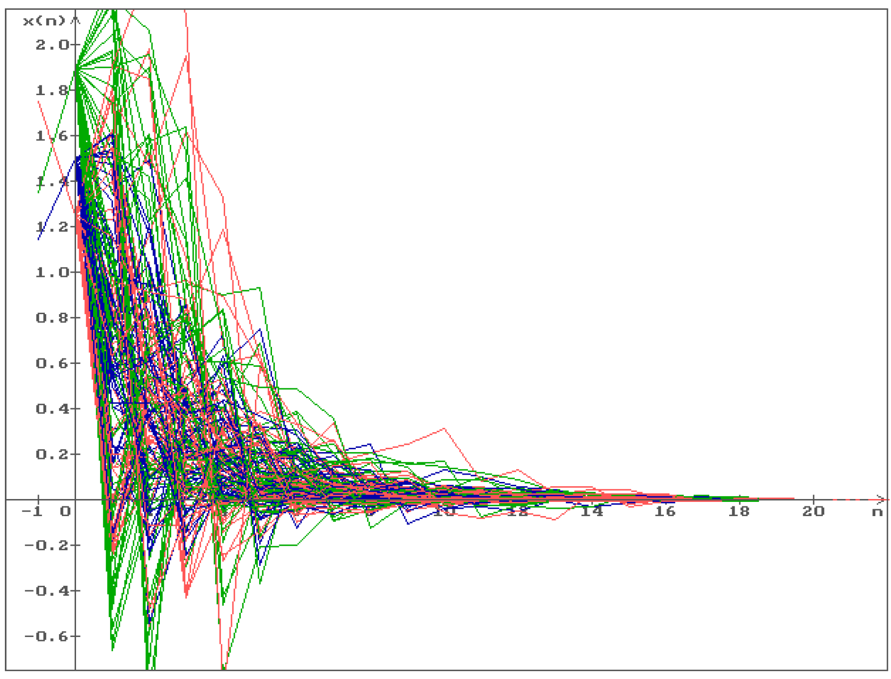
In Figure 1, 50 trajectories of the solution of system (11) are shown ($x_1\left(t\right)$ (blue), $x_2\left(t\right)$ (green), $x_3\left(t\right)$ (red)) with $x_1^{*}=x_2^{*}=x_3^{*}=0$ and the initial conditions:

$$\begin{array}{c}{\phi }_1(-1)=1.15,{\phi }_2(-1)=1.35,{\phi }_3(-1)=1.75,\\ {\phi }_1\left(0\right)=1.5,{\phi }_2\left(0\right)=1.9,{\phi }_3\left(0\right)=1.25.\end{array}$$

One can see that all trajectories converge to the stable zero equilibrium $E_0^{*}(0,0,0)$.

Figure 1. The 50 trajectories of the solution ($x_1\left(n\right)$ (blue), $x_2\left(n\right)$ (green), $x_3\left(n\right)$ (red)) of system (11) converge to the stable zero equilibrium $E_0^{*}(0,0,0)$.

Note that via (7), in this case, all ${\alpha }_i$, $i=1,2,3$, are negative: ${\alpha }_1=-2.9267$, ${\alpha }_2=-1.6582$, and ${\alpha }_3=-2.8904$. Therefore, the conditions (9) do not hold.

Example 2.

Consider again the zero equilibrium $E_0^{*}(0,0,0)$ with the parameter values given in (30) but change only $b_1=0.9$ and $c_2=1$.

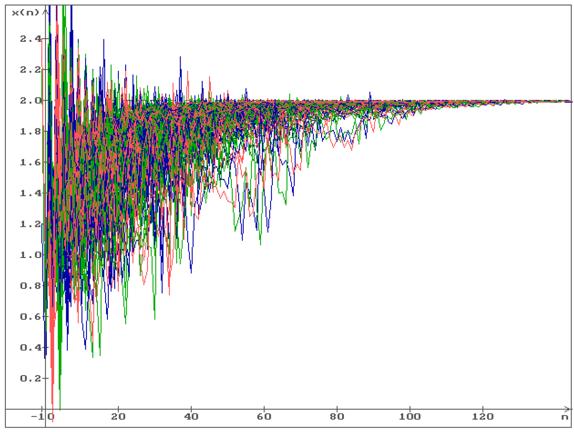
Using MATLAB, it was found that there are no such P and Q matrices for which the LMIs (28) and (29) hold. Via Remark 5, the LMIs (23) and (25)–(27) also do not hold, and equilibrium $E_0^{*}(0,0,0)$ is unstable. In Figure 2, 50 trajectories of the solution of system (11) are shown ($x_1\left(t\right)$ (blue), $x_2\left(t\right)$ (green), $x_3\left(t\right)$ (red)) with $x_1^{*}=x_2^{*}=x_3^{*}=0$, ${\sigma }_1={\sigma }_2={\sigma }_3=0.1$. In addition, the initial conditions that are very close to the zero equilibrium $E_0^{*}(0,0,0)$ are as follows:

$$\begin{array}{c}{\phi }_1(-1)=0.015,{\phi }_2(-1)=-0.01,{\phi }_3(-1)=-0.01,\\ {\phi }_1\left(0\right)=0,{\phi }_2\left(0\right)=0,{\phi }_3\left(0\right)=0.\end{array}$$

One can see that all trajectories leave the unstable equilibrium $E_0^{*}(0,0,0)$.

Figure 2. The 50 trajectories of the solution ($x_1\left(n\right)$ (blue), $x_2\left(n\right)$ (green), $x_3\left(n\right)$ (red)) of system (11) leave the unstable zero equilibrium $E_0^{*}(0,0,0)$.

Note that, via (7), in this case, ${\alpha }_3=0.2231$ is positive, but ${\alpha }_1$ and ${\alpha }_2$ remain negative as in the previous example; therefore, the conditions (9) do not hold.

Example 3.

Put

$$\begin{array}{c}{a}_1=0.1,b_1=0.7,c_1=0.3,\\ a_2=0.2,b_2=0.7,c_2=0.2,\\ a_3=0.3,b_3=0.7,c_3=0.1.\end{array}$$

(31)

Via (4) and Remark 1, the positive equilibrium $E_{+}^{*}(2,2,2)$ exists with

$${\mu }_1=0.0527,{\mu }_2=0.0589,{\mu }_3=0.0668.$$

(32)

From (7), we obtain

$${\alpha }_1=-2.0794,{\alpha }_2=-1.0986,{\alpha }_3=-1.6376,$$

(33)

i.e., the conditions (9) do not hold.

The above means that the inequalities in (9) are sufficient, but not necessary, conditions for the existence of a positive equilibrium of system (1).

Using MATLAB, it was shown, that for the values of the parameters, given in (31), (32), for the positive equilibrium $E_{+}^{*}(2,2,2)$ the LMI (17) holds by ${\sigma }_1=0.29$, ${\sigma }_2=0.32$ and ${\sigma }_3=0.26$ with the following matrices P and Q:

$$P=\left(\begin{array}{ccc}715.50& 372.43& 508.58\\ 372.43& 620.72& 515.25\\ 508.58& 515.25& 917.98\end{array}\right),Q=\left(\begin{array}{ccc}576.19& 319.71& 425.62\\ 319.71& 411.99& 332.77\\ 425.62& 332.77& 483.13\end{array}\right).$$

In Figure 3, 50 trajectories of the solution ($x_1\left(t\right)$ (blue), $x_2\left(t\right)$ (green), $x_3\left(t\right)$ (red)) of system (11) are shown with $x_1^{*}=x_2^{*}=x_3^{*}=2$ and the initial conditions:

$$\begin{array}{c}{\phi }_1(-1)=1.2,{\phi }_2(-1)=2.2,{\phi }_3(-1)=2.4,\\ {\phi }_1\left(0\right)=0.2,{\phi }_2\left(0\right)=0.4,{\phi }_3\left(0\right)=0.9.\end{array}$$

One can see that all trajectories converge to the stable positive equilibrium $E_{+}^{*}(2,2,2)$.

Figure 3. The 50 trajectories of the solution ($x_1\left(n\right)$ (blue), $x_2\left(n\right)$ (green), $x_3\left(n\right)$ (red)) of system (11) converge to the stable positive equilibrium $E_{+}^{*}(2,2,2)$.

Example 4.

Consider now the example with a negative equilibrium. Put

$$\begin{array}{c}{a}_1=0.3,b_1=0.1,c_1=0.3,\\ a_2=0.4,b_2=0.2,c_2=0.2,\\ a_3=0.5,b_3=0.3,c_3=0.1.\end{array}$$

(34)

Via (4) and Remark 1, the negative equilibrium $E_{-}^{*}(-1,-1,-1)$ exists with

$${\mu }_1=0.5596,{\mu }_2=0.4055,{\mu }_3=0.2231.$$

(35)

From (7), we obtain

$${\alpha }_1=-2.7081,{\alpha }_2=-1.3581,{\alpha }_3=-3.0445,$$

that appropriates to the conditions (8).

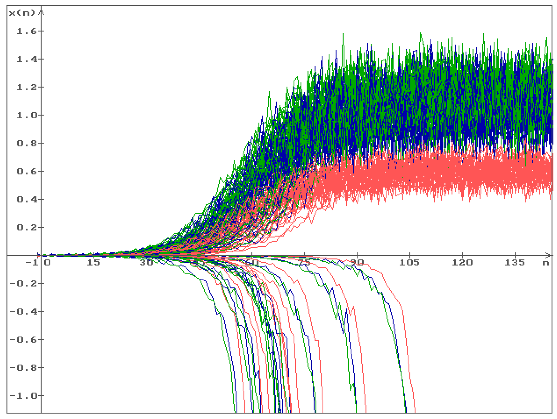
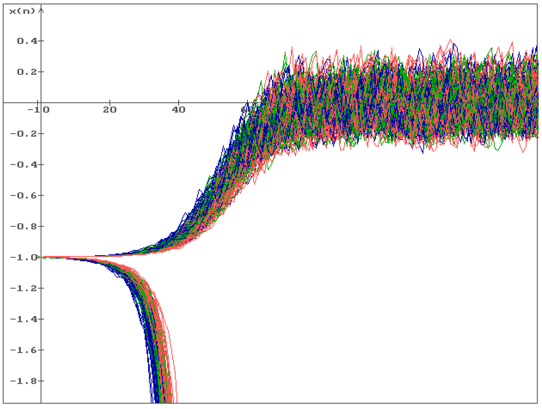
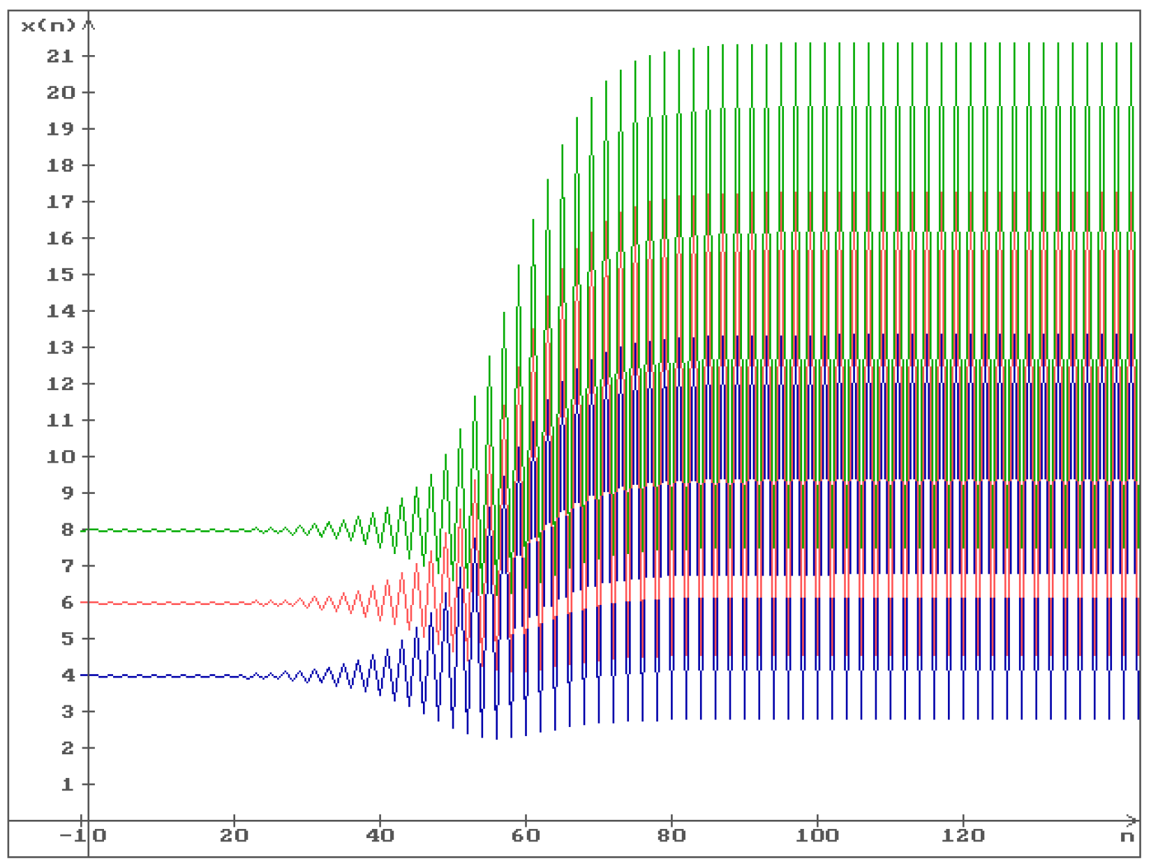
Via MATLAB, it was shown that, with the parameter values given in (34) and (35), the LMIs (28) and (29) did not hold and the negative equilibrium $E_{-}^{*}(-1,-1,-1)$ was unstable even in the deterministic case. In Figure 4, 50 trajectories of the solution of system (11) are shown ($x_1\left(t\right)$ (blue), $x_2\left(t\right)$ (green), and $x_3\left(t\right)$ (red)) with $x_1^{*}=x_2^{*}=x_3^{*}=-1$ and ${\sigma }_1={\sigma }_2={\sigma }_3=0.1$. For the initial conditions that are very close to the equilibrium $E_{-}^{*}(-1,-1,-1)$, we have the following:

$$\begin{array}{c}{\phi }_1(-1)=-1.001,{\phi }_2(-1)=-0.99,{\phi }_3(-1)=-1.001,\\ {\phi }_1\left(0\right)=-1,{\phi }_2\left(0\right)=-1,{\phi }_3\left(0\right)=-1,\end{array}$$

all trajectories oscillate around the zero. After slightly changing the initial conditions ${\phi }_1(-1)=-1.01$ and ${\phi }_3(-1)=-1.01$, while keeping all others, all trajectories go to $-\infty$.

Figure 4. Unstable negative equilibrium $E_{-}^{*}(-1,-1,-1)$. The 50 trajectories of the solution ($x_1\left(n\right)$ (blue), $x_2\left(n\right)$ (green), $x_3\left(n\right)$ (red)) of system (11) oscillate around zero. Moreover, the 50 trajectories go to $-\infty$.

Example 5.

Changing in (31) $c_3=0.1$ on $c_3=0.9$ and using the same values of all other parameters in (31) and (32), we obtain the new positive equilibrium $E_{+}^{*}(5.265,5.686,7.580)$. Via MATLAB, it was shown that, for this positive equilibrium, the LMI (23) holds for ${\sigma }_1=0.32$, ${\sigma }_2=0.33$ and ${\sigma }_3=0.39$ with the following matrices P and Q:

$$P=\left(\begin{array}{ccc}11.145& 2.276& -0.685\\ 2.276& 15.638& 1.465\\ -0.685& 1.465& 13.232\end{array}\right),Q=\left(\begin{array}{ccc}2.886& -0.954& -1.232\\ -0.954& 3.152& -0.696\\ -1.232& -0.696& 2.438\end{array}\right).$$

In Figure 5, 50 trajectories of the solution of system (11) are shown ($x_1\left(t\right)$ (blue), $x_2\left(t\right)$ (green), $x_3\left(t\right)$ (red)) with $x_1^{*}=5.265$, $x_2^{*}=5.686$, $x_3^{*}=7.580$ and the initial conditions:

$$\begin{array}{c}{\phi }_1(-1)=1,{\phi }_2(-1)=2.5,{\phi }_3(-1)=7.5,\\ {\phi }_1\left(0\right)=6,{\phi }_2\left(0\right)=7.5,{\phi }_3\left(0\right)=2.5.\end{array}$$

One can see that all trajectories converge to the stable positive equilibrium $E_{+}^{*}(5.265,5.686,7.580)$.

Figure 5. The 50 trajectories of the solution ($x_1\left(n\right)$ (blue), $x_2\left(n\right)$ (green), $x_3\left(n\right)$ (red)) of system (11) converge to the stable positive equilibrium $E_{+}^{*}(5.265,5.686,7.580)$.

Note that, after increasing $c_3$, we obtain ${\alpha }_1=0.1178>0$, two other ${\alpha }_i$, $i=2,3$, remain negative (see (33)).

Example 6.

In addition to $c_3=0.9$, let us put also $c_1=0.9$ and $c_2=1.1$. In addition, putting ${\mu }_1=1.5163$, ${\mu }_2=0.3466$, and ${\mu }_3=0.0581$, as well as using the same values of the parameters $a_i$ and $b_i$ as in (31), we obtain the new positive equilibrium $E_{+}^{*}(1,2,3)$.

Via MATLAB, it was shown, that for this positive equilibrium LMIs (28) and (29) do not hold. Furthermore, equilibrium $E_{+}^{*}(1,2,3)$ is unstable even in the deterministic case (see Remark 5). In Figure 6, the solution of system (1) is shown ($x_1\left(t\right)$ (blue), $x_2\left(t\right)$ (green), $x_3\left(t\right)$ (red)) with the initial conditions

$$\begin{array}{c}{\phi }_1(-1)=1.001,{\phi }_2(-1)=1.999,{\phi }_3(-1)=3.001,\\ {\phi }_1\left(0\right)=1,{\phi }_2\left(0\right)=2,{\phi }_3\left(0\right)=3,\end{array}$$

which are close to the equilibrium $E_{+}^{*}(1,2,3)$. One can see that this equilibrium is unstable and that the solution leaves the equilibrium.

Figure 6. The solution ($x_1\left(n\right)$ (blue), $x_2\left(n\right)$ (green), $x_3\left(n\right)$ (red)) of system (11) with the unstable positive equilibrium $E_{+}^{*}(1,2,3)$. The solution leaves the equilibrium.

Note that, in this case, all ${\alpha }_i$, $i=1,2,3$ are non-negative: ${\alpha }_1=0.1178>0$, ${\alpha }_2=0$, and ${\alpha }_3=0.0671>0$.

Example 7.

Putting $a_1=a_2=a_3=0.2$, $b_1=b_2=b_3=c_1=c_2=c_3=0.8$, ${\mu }_1=0.3132$, ${\mu }_2=0.0279$, and ${\mu }_3=0.1155$, we obtain the new positive equilibrium $E_{+}^{*}(4,8,6)$.

Via MATLAB, it was shown, that for this positive equilibrium LMIs (28) and (29) do not hold, and equilibrium $E_{+}^{*}(4,8,6)$ is unstable even in the deterministic case. In Figure 7, the solution ($x_1\left(t\right)$ (blue), $x_2\left(t\right)$ (green), $x_3\left(t\right)$ (red)) of system (1) is shown with the initial conditions

$$\begin{array}{c}{\phi }_1(-1)=4.01,{\phi }_2(-1)=7.999,{\phi }_3(-1)=6.01,\\ {\phi }_1\left(0\right)=4,{\phi }_2\left(0\right)=8,{\phi }_3\left(0\right)=6,\end{array}$$

which are close to the equilibrium $E_{+}^{*}(4,8,6)$. One can see that this equilibrium is unstable and that the solution leaves the equilibrium. Note that, in this case, ${\alpha }_1={\alpha }_2={\alpha }_3=0$.

Figure 7. The solution ($x_1\left(n\right)$ (blue), $x_2\left(n\right)$ (green), $x_3\left(n\right)$ (red)) of system (11) with the unstable positive equilibrium $E_{+}^{*}(4,8,6)$. The solution leaves the equilibrium.

Remark 7.

Note that positive equilibria are considered in Examples 3 and 5–7. In Examples 6 and 7, all ${\alpha }_i$ are non-negative and both equilibria are unstable. In Examples 3 and 5, there is negative ${\alpha }_i$, and both equilibria are stable. In this regard, the following open problem arises.

The open problem. Prove or disprove the following statement: “If for a given set of parameters all conditions (9) hold, i.e., all ${\alpha }_i$, $i=1,2,3$, defined in (7), are non-negative, then the positive equilibrium obtained by this set of parameters is unstable”.

5. Combination of Exponential and Fractional Nonlinearities

Consider the system of m difference equations with exponential and fractional nonlinearities

$$\begin{array}{c}\begin{array}{c}{x}_k(n+1)=\frac{{\alpha }_k+{\beta }_k{e}^{-f_k\left(x(n-1)\right)}}{{\gamma }_k+g_k\left(x\left(n\right)\right)},n\in N,\\ x_k\left(j\right)={\varphi }_k\left(j\right),j\in N_0,k=1,\dots ,m,\end{array}\hfill \end{array}$$

(36)

where

$$\begin{array}{c}\begin{array}{c}x=(x_1,\dots ,x_m),f_k\left(x\right)={\displaystyle \sum _{i=1}^m}{\mu }_{ki}{x}_i,g_k\left(x\right)={\displaystyle \sum _{i=1}^m}{\nu }_{ki}{x}_i,\end{array}\hfill \end{array}$$

(37)

the parameters ${\alpha }_k$, ${\beta }_k$ and ${\gamma }_k$ are positive numbers, ${\mu }_{ki}$, ${\nu }_{ki}$ and the initial conditions ${\varphi }_k\left(j\right)$ are non-negative numbers.

Equations of this type are found in the research [4,5]. Different particular cases of system (36), (37) were considered in [33,34]. Let, for instance, $m=2$. Putting ${\mu }_{12}={\mu }_{21}={\nu }_{11}={\nu }_{22}=0$, from (36) and (37) we obtain

$$\begin{array}{c}{x}_1(n+1)={\displaystyle \frac{{\alpha }_1+{\beta }_1{e}^{-{\mu }_{11}{x}_1(n-1)}}{{\gamma }_1+{\nu }_{12}{x}_2\left(n\right)}},\hfill \\ x_2(n+1)={\displaystyle \frac{{\alpha }_2+{\beta }_2{e}^{-{\mu }_{22}{x}_2(n-1)}}{{\gamma }_2+{\nu }_{21}{x}_1\left(n\right)}},n\in N.\hfill \end{array}$$

(38)

Putting ${\mu }_{11}={\mu }_{22}={\nu }_{11}={\nu }_{22}=0$, we, similarly, have

$$\begin{array}{c}{x}_1(n+1)={\displaystyle \frac{{\alpha }_1+{\beta }_1{e}^{-{\mu }_{12}{x}_2(n-1)}}{{\gamma }_1+{\nu }_{12}{x}_2\left(n\right)}},\hfill \\ x_2(n+1)={\displaystyle \frac{{\alpha }_2+{\beta }_2{e}^{-{\mu }_{21}{x}_1(n-1)}}{{\gamma }_2+{\nu }_{21}{x}_1\left(n\right)}},n\in N.\hfill \end{array}$$

(39)

The solution $x\left(n\right)=(x_1\left(n\right),\dots ,x_m\left(n\right))=(x_1^{*},\dots ,x_m^{*})=x^{*}$ is the equilibrium of system (36), and it is defined by the system of the equations

$$x_k^{*}=\frac{{\alpha }_k+{\beta }_k{e}^{-f_k\left(x^{*}\right)}}{{\gamma }_k+g_k\left(x^{*}\right)},k=1,\dots ,m.$$

(40)

Remark 8.

By presenting Equation (40) in the form

$$x_k^{*}\left({\gamma }_k+g_k\left(x^{*}\right)\right)={\alpha }_k+{\beta }_k{e}^{-f_k\left(x^{*}\right)},$$

it is easy to see that the left part of this equation for each $x_k^{*}$ increases from the zero to the infinity, whereas the right part does not increase. Therefore, Equation (40) has a unique positive solution.

Below the stability of the equilibrium of system (36) is studied under stochastic perturbations that are proportional to the deviation of the system state $x\left(n\right)$ from the system equilibrium $x^{*}$.

Similar to (11) and (10), let us assume that system (36) is exposed to stochastic perturbations that are directly proportional to the deviation of the current value of the system solution from its equilibrium, i.e.,

$$\begin{array}{c}\begin{array}{cc}\hfill x_k(n+1)& =\frac{{\alpha }_k+{\beta }_k{e}^{-f_k\left(x(n-1)\right)}}{{\gamma }_k+g_k\left(x\left(n\right)\right)}+{\sigma }_k(x_k\left(n\right)-x_k^{*}){\xi }_k(n+1),n\in N,\hfill \\ \hfill x_k\left(j\right)& ={\varphi }_k\left(j\right),j\in N_0,k=1,\dots ,m.\hfill \end{array}\hfill \end{array}$$

(41)

By putting in (41) $x_k\left(n\right)=y_k\left(n\right)+x_k^{*}$, we obtain

$$y_k(n+1)+x_k^{*}=\frac{{\alpha }_k+{\beta }_k{e}^{-f_k(y(n-1)+x^{*})}}{{\gamma }_k+g_k(y\left(n\right)+x^{*})}+{\sigma }_k{y}_k\left(n\right){\xi }_k(n+1).$$

(42)

Note that via (37), we have

$$f_k(y+x^{*})=f_k\left(y\right)+f_k\left(x^{*}\right),g_k(y+x^{*})=g_k\left(y\right)+g_k\left(x^{*}\right).$$

(43)

Substituting (43) into (42) gives

$$\begin{array}{c}\begin{array}{cc}\hfill y_k(n+1)+x_k^{*}& =\frac{{\alpha }_k+{\beta }_k{e}^{-f_k\left(x^{*}\right)}{e}^{-f_k\left(y(n-1)\right)}}{{\gamma }_k+g_k\left(x^{*}\right)+g_k\left(y\left(n\right)\right)}+{\sigma }_k{y}_k\left(n\right){\xi }_k(n+1),\hfill \\ \hfill k& =1,\dots ,m.\hfill \end{array}\hfill \end{array}$$

(44)

Via (40), it is clear that system (44) has the zero solution.

Using the simple equalities

$$e^{-z}=1-z+o\left(z\right),\frac{1}{a+z}=\frac{1}{a}-\frac{z}{a^2}+o\left(z\right),\underset{z\to 0}{lim}\frac{o\left(z\right)}{z}=0,$$

and (40), we have

$$\begin{array}{c}\begin{array}{c}\frac{{\alpha }_k+{\beta }_k{e}^{-f_k\left(x^{*}\right)}{e}^{-f_k\left(y(n-1)\right)}}{{\gamma }_k+g_k\left(x^{*}\right)+g_k\left(y\left(n\right)\right)}\hfill \\ =[{\alpha }_k+{\beta }_k{e}^{-f_k\left(x^{*}\right)}(1-f_k\left(y(n-1)\right)+o\left(y\right))]\left[\frac{1}{{\gamma }_k+g_k\left(x^{*}\right)}-\frac{g_k\left(y\left(n\right)\right)}{{({\gamma }_k+g_k\left(x^{*}\right))}^2}+o\left(y\right)\right]\hfill \\ =x_k^{*}-a_k{g}_k\left(y\left(n\right)\right)-b_k{f}_k\left(y(n-1)\right)+o\left(y\right),\hfill \end{array}\hfill \end{array}$$

(45)

where

$$\begin{array}{c}{a}_k={\displaystyle \frac{{\alpha }_k+{\beta }_k{e}^{-f_k\left(x^{*}\right)}}{{({\gamma }_k+g_k\left(x^{*}\right))}^2}},b_k={\displaystyle \frac{{\beta }_k{e}^{-f_k\left(x^{*}\right)}}{{\gamma }_k+g_k\left(x^{*}\right)}}.\hfill \end{array}$$

(46)

By substituting (45) into (44), we have

$$y_k(n+1)=-a_k{g}_k\left(y\left(n\right)\right)-b_k{f}_k\left(y(n-1)\right)+o\left(y\right)+{\sigma }_k{y}_k\left(n\right){\xi }_k(n+1).$$

(47)

Rejecting nonlinear terms in (47) and using (37), we obtain the linear part of Equation (47)

$$z_k(n+1)=-a_k{\displaystyle \sum _{j=1}^m}{\nu }_{kj}{z}_j\left(n\right)-b_k{\displaystyle \sum _{j=1}^m}{\mu }_{kj}{z}_j(n-1)+{\sigma }_k{z}_k\left(n\right){\xi }_k(n+1)$$

and rewrite it in the matrix form

$$\begin{array}{cc}\hfill z(n+1)& =-Az\left(n\right)-Bz(n-1)+{\displaystyle \sum _{k=1}^m}{C}_{k}z\left(n\right){\xi }_k(n+1),n\in N,\hfill \\ \hfill z\left(j\right)& =\varphi \left(j\right),j\in N_0,\hfill \end{array}$$

(48)

where A and B are the $m\times m$-matrices with the elements $a_k{\nu }_{ki}$ and $b_k{\mu }_{ki}$ respectively, $k,i=1,\dots ,m$, $a_k$ and $b_k$ are defined in (46), $C_k$ is an $m\times m$-matrix with all zero elements instead of $c_{kk}={\sigma }_k$, $k=1,\dots ,m$.

5.1. Stability Conditions

Here, via the general method of Lyapunov functional construction [12,13] and the method of linear matrix inequalities (LMIs) [19,20,21,22,23,24,25,26,27], the conditions for stability in the probability of the equilibrium of system (41) are obtained.

Theorem 5.

Let for the matrices A, B and $C_k$ of equation (48) there exist positive definite $m\times m$-matrices P and R, such that the LMI

$$\left[\begin{array}{cc}{A}^{\prime }PA+B^{\prime }PB-P+A^{\prime }RA+{\displaystyle \sum _{k=1}^m}{C}_k^{\prime }P{C}_k& B^{\prime }P\\ PB& -R\end{array}\right]<0$$

(49)

holds. Then, the equilibrium $x^{*}$ of system (41) is stable in probability.

Proof. 

Following the general method of Lyapunov functional construction [12,13], consider the Lyapunov functional $V\left(n\right)$ in the form $V\left(n\right)=V_1\left(n\right)+V_2\left(n\right)$, where $V_1\left(n\right)=z^{\prime }\left(n\right)Pz\left(n\right)$, $P>0$, and the additional functional $V_2\left(n\right)$ will be chosen below. Then

$$\begin{array}{cc}\mathbf{E}\Delta V_1\left(n\right)\hfill & =\mathbf{E}(V_1(n+1)-V_1\left(n\right))\hfill \\ \hfill & =\mathbf{E}\left[{\left(-Az\left(n\right)-Bz(n-1)+{\displaystyle \sum _{k=1}^m}{C}_{k}z\left(n\right){\xi }_k(n+1)\right)}^{\prime }P\right.\hfill \\ \hfill & \times \left.\left(-Az\left(n\right)-Bz(n-1)+{\displaystyle \sum _{k=1}^m}{C}_{k}z\left(n\right){\xi }_k(n+1)\right)-z^{\prime }\left(n\right)Pz\left(n\right)\right]\hfill \\ \hfill & =\mathbf{E}[z^{\prime }\left(n\right)\left(A^{\prime }PA-P+{\displaystyle \sum _{k=1}^m}{C}_k^{\prime }P{C}_k\right)z\left(n\right)+z^{\prime }\left(n\right)A^{\prime }PBz(n-1)\hfill \\ \hfill & +z^{\prime }(n-1)B^{\prime }PAz\left(n\right)+z^{\prime }(n-1)B^{\prime }PBz(n-1)].\hfill \end{array}$$

(50)

Using inequality (24) with $a=Az\left(n\right)$, $b=PBz(n-1)$ and the positive definite matrix R, we obtain

$$z^{\prime }\left(n\right)A^{\prime }PBz(n-1)+z^{\prime }(n-1)B^{\prime }PAz\left(n\right)\le z^{\prime }\left(n\right)A^{\prime }RAz\left(n\right)+z^{\prime }(n-1)B^{\prime }P{R}^{-1}PBz(n-1).$$

(51)

Substituting (51) into (50), we obtain

$$\begin{array}{cc}\mathbf{E}\Delta V_1\left(n\right)\hfill & \le \mathbf{E}[z^{\prime }\left(n\right)\left(A^{\prime }PA-P+A^{\prime }RA+{\displaystyle \sum _{k=1}^m}{C}_k^{\prime }P{C}_k\right)z\left(n\right)\hfill \\ \hfill & +z^{\prime }(n-1)B^{\prime }(P{R}^{-1}P+P)Bz(n-1)].\hfill \end{array}$$

(52)

Using now the additional functional $V_2\left(n\right)$ in the form $V_2\left(n\right)=z^{\prime }(n-1)B^{\prime }(P{R}^{-1}P+P)Bz(n-1)$, for the functional $V\left(n\right)=V_1\left(n\right)+V_2\left(n\right)$ we obtain

$$\mathbf{E}\Delta V\left(n\right)\le \mathbf{E}\left[z^{\prime }\left(n\right)Qz\left(n\right)\right],$$

(53)

where

$$Q=A^{\prime }PA+B^{\prime }PB-P+A^{\prime }RA+B^{\prime }P{R}^{-1}PB+{\displaystyle \sum _{k=1}^m}{C}_k^{\prime }P{C}_k.$$

(54)

Via the Schur complement, the matrix (54) is negative definite if and only if the LMI (49) holds. So, the matrix Q is negative definite. Via this and (53), it means that $\mathbf{E}\Delta V\left(n\right)\le -{c\mathbf{E}\left|z\left(n\right)\right|}^2$ for some $c>0$. From Theorem 2, it follows that the zero solution of the Equation (48) is asymptotically mean square stable. Via Remark 3, it means that the equilibrium $x^{*}$ of system (41) is stable in probability. Thus, the proof is completed. □

5.2. Examples

To illustrate the obtained stability conditions, consider the following examples.

Example 8.

By putting in (36) and (37)

$$\begin{array}{c}m=2,{\mu }_{12}={\mu }_{21}={\nu }_{11}={\nu }_{22}=0,\hfill \\ {\mu }_{11}={\mu }_{22}={\nu }_{12}={\nu }_{21}=1,\hfill \\ {\alpha }_1=30,{\beta }_1=1.4,{\gamma }_1=1.5,\hfill \\ {\alpha }_2=45,{\beta }_2=2.5,{\gamma }_2=2.8,\hfill \end{array}$$

(55)

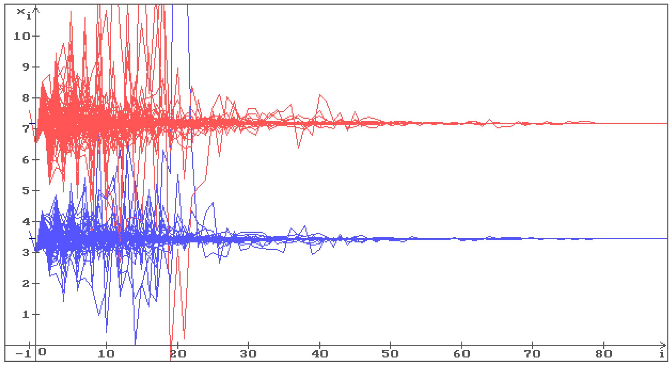
we obtain system (38) with the equilibrium [34]

$$E_1^{*}(x_1^{*},x_2^{*})=(3.455959,7.193442).$$

(56)

After adding stochastic perturbations, system (38) takes the form

$$\begin{array}{cc}{x}_1(n+1)\hfill & ={\displaystyle \frac{{\alpha }_1+{\beta }_1{e}^{-{\mu }_{11}{x}_1(n-1)}}{{\gamma }_1+{\nu }_{12}{x}_2\left(n\right)}}+{\sigma }_1(x_1\left(n\right)-x_1^{*}){\xi }_1(n+1),\hfill \\ x_2(n+1)\hfill & ={\displaystyle \frac{{\alpha }_2+{\beta }_2{e}^{-{\mu }_{22}{x}_2(n-1)}}{{\gamma }_2+{\nu }_{21}{x}_1\left(n\right)}}+{\sigma }_2(x_2\left(n\right)-x_2^{*}){\xi }_2(n+1).\hfill \end{array}$$

(57)

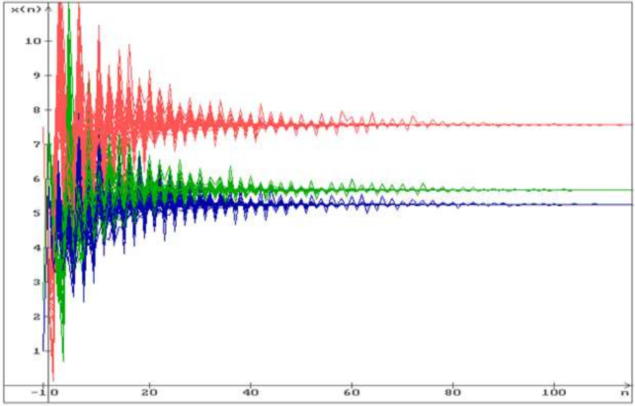
Via MATLAB, it was shown that LMI (49) for system (57) holds with the following maximum noise levels: ${\sigma }_1=0.781$ and ${\sigma }_2=0.674$. In Figure 8, 100 trajectories of system (57) solution are shown by the values of their parameters, which are given in (55) and the initial conditions $x_1(-1)=3.7$, $x_1\left(0\right)=3.0$, $x_2(-1)=7.6$, $x_2\left(0\right)=6.5$, as well as ${\sigma }_1=0.77$ and ${\sigma }_2=0.66$. One can see that all trajectories converge to the stable equilibrium (56).

Figure 8. The 100 trajectories of the solution ($x_1\left(n\right)$ (blue), $x_2\left(n\right)$ (red)) of system (57) converge to the stable equilibrium (56).

Example 9.

By putting in (36) and (37)

$$\begin{array}{c}m=2,{\mu }_{11}={\mu }_{22}={\nu }_{11}={\nu }_{22}=0,\hfill \\ {\mu }_{12}={\nu }_{12}=1/3,{\mu }_{21}={\nu }_{21}=1,\hfill \\ {\alpha }_1=1,{\beta }_1=e,{\gamma }_1=1,\hfill \\ {\alpha }_2=3,{\beta }_2=e,{\gamma }_2=1/3,\hfill \end{array}$$

(58)

we obtain system (39) with the equilibrium

$$E_2^{*}(x_1^{*},x_2^{*})=(1,3).$$

(59)

After adding stochastic perturbation, system (39) takes the form

$$\begin{array}{c}{x}_1(n+1)={\displaystyle \frac{{\alpha }_1+{\beta }_1{e}^{-{\mu }_{12}{x}_2(n-1)}}{{\gamma }_1+{\nu }_{12}{x}_2\left(n\right)}}+{\sigma }_1(x_1\left(n\right)-x_1^{*}){\xi }_1(n+1),\hfill \\ x_2(n+1)={\displaystyle \frac{{\alpha }_2+{\beta }_2{e}^{-{\mu }_{21}{x}_1(n-1)}}{{\gamma }_2+{\nu }_{21}{x}_1\left(n\right)}}+{\sigma }_2(x_2\left(n\right)-x_2^{*}){\xi }_2(n+1).\hfill \end{array}$$

(60)

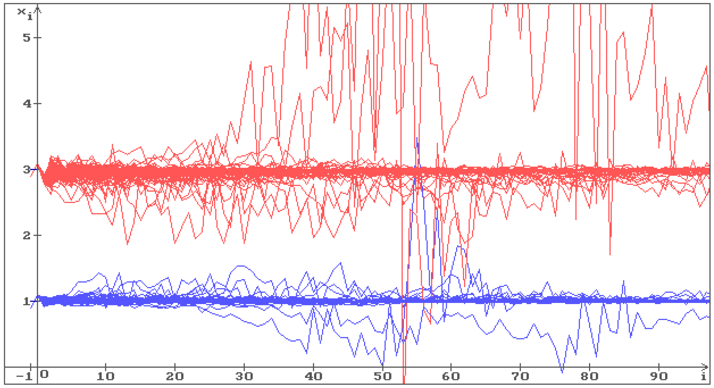
Via MATLAB, it was shown that LMI (49) for system (60) does not hold even in the deterministic case, i.e., for ${\sigma }_1={\sigma }_2=0$. So, the equilibrium (59) is unstable. In Figure 9, 100 trajectories of system (60) solution are shown by the values of the parameters given in (58), the initial conditions $x_1(-1)=0.9$, $x_1\left(0\right)=1.1$, $x_2(-1)=2.9$, $x_2\left(0\right)=3.1$, as well as ${\sigma }_1=0.47$ and ${\sigma }_2=0.48$. One can see that the trajectories do not converge to the equilibrium and fill the whole space.

Figure 9. The 100 trajectories of the solution ($x_1\left(n\right)$ (blue), $x_2\left(n\right)$ (red)) of system (60). The equilibrium (59) is unstable, and the trajectories fill whole space.

6. Conclusions

The method of stability investigation for nonlinear systems under stochastic perturbations is demonstrated through the study of a system of difference equations with exponential nonlinearity, as well as via a system with both exponential and fractional nonlinearities. Conditions of stability in probability for the equilibrium of a system under consideration are obtained, using the general method of Lyapunov functionals construction, are formulated in terms of linear matrix inequalities and are illustrated by numerical examples and figures.

The method of the stability investigation used in the paper can be applied to many other types of nonlinear systems for both difference and differential equations in various applications. For readers, attention is directed to an unsolved problem, the solution of which could provide the method under consideration some additional interesting possibilities.

References

- Ding, X.; Zhang, R. On the difference equation xn+1 = (αxn + βxn−1)e−xn. Adv. Differ. Equ. 2008, 2008, 876936. [Google Scholar] [CrossRef][Green Version]
- Ding, X.; Li, W. Stability and bifurcation of numerical discretization Nicholson blowflies equation with delay. Discret. Dyn. Nat. Soc. 2006, 2006, 019413. [Google Scholar] [CrossRef]
- El-Metwally, H.; Grove, E.A.; Ladas, G.; Levins, R.; Radin, M. On the difference equation xn+1 = α + βxn−1e−xn. Nonlinear Anal. Theory Methods Appl. 2001, 47, 4623–4634. [Google Scholar] [CrossRef]
- Ozturk, I.; Bozkurt, F.; Ozen, S. On the difference equation . Appl. Math. Comput. 2006, 181, 1387–1393. [Google Scholar] [CrossRef]
- Ozturk, I.; Bozkurt, F.; Ozen, S. Global asymptotic behavior of the difference equations: . Appl. Math. Lett. 2009, 22, 595–599. [Google Scholar] [CrossRef]
- Papaschinopoulos, G.; Radin, M.A.; Schinas, C.J. On the system of two difference equations of exponential form: xn+1 = a + bxn−1e−yn, yn+1 = c + dyn−1e−xn. Math. Comput. Model. 2011, 54, 2969–2977. [Google Scholar] [CrossRef]
- Papaschinopoulos, G.; Radin, M.A.; Schinas, C.J. Study of the asymptotic behavior of the solutions of three systems of difference equations of exponential form. Appl. Math. Comput. 2012, 218, 5310–5318. [Google Scholar] [CrossRef]
- Papaschinopoulos, G.; Fotiades, N.; Schinas, C.J. On a system of difference equations including negative exponential terms. J. Differ. Equ. Appl. 2014, 20, 717–732. [Google Scholar] [CrossRef]
- Papaschinopoulos, G.; Ellina, G.; Papadopoulos, K.B. Asymptotic behavior of the positive solutions of an exponential type system of difference equations. Appl. Math. Comput. 2014, 245, 181–190. [Google Scholar] [CrossRef]
- Shaikhet, L. Stability of equilibrium states for a stochastically perturbed Mosquito population equation. Dyn. Contin. Discret. Impuls. Syst. B Appl. Algorithms 2014, 21, 185–196. [Google Scholar]
- Shaikhet, L. Stability of equilibrium states for a stochastically perturbed exponential type system of difference equations. J. Comput. Appl. Math. 2015, 290, 92–103. [Google Scholar] [CrossRef]
- Shaikhet, L. Lyapunov Functionals and Stability of Stochastic Difference Equations; Springer Science & Business Media: London, UK, 2011. [Google Scholar]
- Shaikhet, L. Lyapunov Functionals and Stability of Stochastic Functional Differential Equations; Springer Science & Business Media: Berlin, Germany, 2013. [Google Scholar]
- Lakshmikantham, V.; Trigiante, D. Theory of Difference Equations: Numerical Methods and Applications; Academic Press: New York, NY, USA, 1988. [Google Scholar]
- Kocic, V.L.; Ladas, G. Global Behaviour of Nonlinear Difference Equations of HIGHER order with Applications; Mathematics and its applications, Volume 256; Kluwer Academic: Dordrecht, The Netherlands, 1993. [Google Scholar]
- Agarwal, R.P.; Wong, P.J.Y. Advanced Topics in Difference Equations; Mathematics and its applications, Volume 404; Kluwer Academic: Dordrecht, The Netherlands, 1997. [Google Scholar]
- Kulenovic, M.R.S.; Ladas, G. Dynamics of Second Order Rational Difference Equations, Open Problems and Conjectures; Chapman & Hall/CRC: Boca Raton, FL, USA, 2002. [Google Scholar]
- Elaydi, S. An Introduction to Difference Equations, 3rd ed.; Springer: Berlin, Germany, 2005. [Google Scholar]
- Boyd, S.; El-Ghaoui, L.; Feron, E.; Balakrishnan, V. Linear Matrix Inequalities in System and Control Theory; SIAM: Philadelphia, PA, USA, 1994. [Google Scholar]
- Choi, H.H. A new method for variable structure control system design: A linear matrix inequality approach. Automatica 1997, 33, 2089–2092. [Google Scholar] [CrossRef]
- Niculescu, S.I. H∞ memory less control with an α-stability constraint for time delays systems: An LMI approach. IEEE Trans. Autom. Control 1998, 43, 739–743. [Google Scholar] [CrossRef]
- Nguang, S.K. Robust H∞ control of a class of nonlinear systems with delayed state and control: An LMI approach. In Proceedings of the 37th IEEE Conference on Decision and Control, Tampa, FL, USA, 16–18 December 1998; pp. 2384–2389. [Google Scholar]
- Gouaisbaut, F.; Dambrine, M.; Richard, J.P. Robust control of delay systems: A sliding mode control design via LMI. Syst. Control Lett. 2002, 46, 219–230. [Google Scholar] [CrossRef]
- Seuret, A.; Gouaisbaut, F. Hierarchy of LMI conditions for the stability analysis of time-delay systems. Syst. Control Lett. 2015, 81, 1–7. [Google Scholar] [CrossRef]
- Fridman, E.; Shaikhet, L. Stabilization by using artificial delays: An LMI approach. Automatica 2017, 81, 429–437. [Google Scholar] [CrossRef]
- Fridman, E.; Shaikhet, L. Delay-dependent LMI conditions for stability of stochastic systems with delay term in the form of Stieltjes integral. In Proceedings of the 57th IEEE Conference on Decision and Control, Fontainebleau, Miami Beach, FL, USA, 17–18 December 2018; pp. 6567–6572. [Google Scholar]
- Fridman, E.; Shaikhet, L. Simple LMIs for stability of stochastic systems with delay term given by Stieltjes integral or with stabilizing delay. Syst. Control Lett. 2019, 124, 83–91. [Google Scholar] [CrossRef]
- Shaikhet, L. About one method of stability investigation for nonlinear stochastic delay differential equations. Int. J. Robust Nonlinear Control 2021, 31, 2946–2959. [Google Scholar] [CrossRef]
- Shaikhet, L. Some generalization of the method of stability investigation for nonlinear stochastic delay differential equations. Symmetry 2022, 14, 1734. [Google Scholar] [CrossRef]
- Shaikhet, L. Stability of equilibria of exponential type system of three differential equations under stochastic perturbations. Math. Comput. Simul. 2023, 206, 105–117. [Google Scholar] [CrossRef]
- Beretta, E.; Kolmanovskii, V.; Shaikhet, L. Stability of epidemic model with time delays influenced by stochastic perturbations. Math. Comput. Simul. 1998, 45, 269–277. [Google Scholar] [CrossRef]
- Haynsworth, E.V. On the Schur complement. Basel Math. Notes 1968, 20, 17. [Google Scholar]
- Thai, T.H.; Dai, N.A.; Anh, P.T. Global dynamics of some system of second-order difference equations. Electron. Res. Arch. 2021, 29, 4159–4175. [Google Scholar] [CrossRef]
- Khan, A.Q. Global Dynamics of a Nonsymmetric System of Difference Equations. Math. Probl. Eng. 2022, 2022, 4435613. [Google Scholar] [CrossRef]
Disclaimer/Publisher’s Note: The statements, opinions and data contained in all publications are solely those of the individual author(s) and contributor(s) and not of MDPI and/or the editor(s). MDPI and/or the editor(s) disclaim responsibility for any injury to people or property resulting from any ideas, methods, instructions or products referred to in the content. |
© 2023 by the author. Licensee MDPI, Basel, Switzerland. This article is an open access article distributed under the terms and conditions of the Creative Commons Attribution (CC BY) license (https://creativecommons.org/licenses/by/4.0/).