Abstract
In this paper, a new type of one-degree-of-freedom pure nonlinear oscillator with a time variable degree of nonlinearity is introduced. Namely, the degree of the nonlinearity in the restitution force is not a constant but a ‘slow time’ variable function. The mathematical model is a second-order nonlinear differential equation with time-variable parameters. An approximate solving procedure based on the method of time-variable amplitude, frequency and phase is developed. It is found that the vibration properties depend on initial conditions and the degree of time-variable function. The theoretical results are tested on almost linear, cubic and high-degree nonlinear oscillators. According to theoretical considerations, the process of aging in fiber-reinforced polymer composite structure is investigated. It is found that the amplitude and the frequency of vibration of the reinforced polymer structure decrease over time. The result is in good agreement with already published experimental data. The additional conclusion of the research is that the oscillator model suggested in the paper is suitable for the prediction of mechanic properties of the polymer structure in aging and also in similar destructive processes.
Keywords:
aging in fiber-reinforced polymer composite; analytic solving procedure; Ateb function; nonlinear oscillator; time-variable nonlinearity; marine industry MSC:
34C15
1. Introduction
The dynamics of the mass variable system have a long history. Its main significance is in rocket theory, but recently, it has been applied in machines, mechanisms and processes where mass varies over time. Thus, it is utilized in the dynamics of machines in cable, paper, and textile industries where the mass of the drum varies over time [1] but also in the determination of dynamic characteristics in the movement of vehicles and wheeled tractors with units of variable mass [2]. It is found that due to mass variation, a reactive force occurs, which affects the motion of the system [3]. In the machining of the workpiece by turning, the vibrations are caused by mass variation. Namely, during the action of moving the cutting force in the turning processing, the mass of the workpiece changes due to chip loss. It causes the workpiece to vibrate [4]. The time-varying mass makes the natural frequency of the system no longer constant but dependent on the workpiece mass. There are also a significant number of mechanisms with variable mass. Let us mention the variable mass system of the maglev turning electric spindle [5]. Research in the dynamics of the mechanism requires the consideration of the mass variable model. Mass variation is evident in the various processes. Determination of blasting load in boreholes is possible based on a variable mass thermodynamic system [6]. The problem of non-linear porous sublimation with temperature-dependent thermal conductivity and concentration-dependent mass diffusivity [7] requires the application of the dynamics of a mass variable system.
In addition, variable mass dynamics is suitable for designing new vibration-damping equipment. Let us mention some of them: a variable mass negative stiffness dynamic vibration absorber [8], a non-piston MR suspension rod for variable mass systems [9], the variable mass pendulum type assembly for damping [10], etc. In [11], the self-adjustable tuned mass damper with variable mass is studied. It is shown that it is suitable as an adaptive passive variable mass tuned mass damper [12]. Namely, the adaptive-passive variable mass tuned mass damper can retune itself through varying its mass. Wang et al. [13] state that the damper is a contribution to the traditional one used in vertical vibration control of footbridges. A large-span floor structure is proposed as a case study. In [14], it is shown that the innovative adaptive tuned vibration absorber with a variable mass moment of inertia is suitable for the mitigation of the transient response of systems. The adaptive passive variable mass tuned mass damper can control human-induced vertical vibrations. For passive vibration control of the variable mass structure, a novel tuned mass-conical spring system is designed [15]. The principle of the damper is in the context of a varying mass system. The conical spring-tuned mass damper remains tuned and thereby achieves significant response reductions under the stiffening conditions of the primary structure. The advantage of the damper in comparison to the linear spring-tuned mass damper is that the latter suffers performance degradation because of detuning whenever there is any fluctuation in the system mass.
In the previously mentioned research, various types of models for the mass variable system are developed. In general, the model is the one-degree-of-freedom nonlinear oscillator with time-variable parameters and is convenient for the description of the dynamics of systems and processes varying over time. The corresponding mathematical model is
where is the restitution force function, and is the function of additional forces (damping, friction, aerodynamic, excitation, etc.), x is the displacement, t is real time, and is the ‘slow time’. The slow time is the product of the real time t and a small parameter ε < < 1, i.e., , Usually, the restitution force function is a nonlinear polynomial function F(x). However, in the oscillator where geometric characteristics (length, dimensions) and physical properties (mass, for example) are varying slowly over time, the force function is dependent not only on displacement x but also on the slow time τ, i.e., In the model of the force, the coefficient of elasticity is assumed to be a slow time-variable function, and the elastic force is modeled as the product of the time-variable parameter and nonlinear displacement function . However, the suggested and already developed model (1) is not convenient for the description of the time-variable restitution force, where the variation is caused by some processes, for example, the aging of the material and structure (see for example [16,17]). Namely, in these processes, the coefficient of nonlinearity is not time dependent, but the degree of nonlinearity varies over time. To overcome the lack of known models and to explain the mentioned phenomena, a new model, where the degree of nonlinearity is the time-variable function, is necessary to be developed.
The new model, the oscillator, where the degree of nonlinearity of the restitution force varies over time, is considered. It is assumed that the coefficient of elasticity is constant, but the degree of nonlinearity is the function of the ‘slow time’ τ. The model of the oscillator is a second order differential equation with a time-variable degree of nonlinearity. For solving the model, a new procedure, based on the ‘Cveticanin’s method’ [18] and Ateb function (the inverse complete Beta function) [19], is developed. It is found that the computed amplitude and frequency of vibration are time-variable functions. They depend also on the initial conditions.
In this paper, the amplitude and frequency solutions are analyzed and discussed. The new analytical procedure and the obtained solution and result are tested for the aging process of fiber-reinforced polymer composite. The analytic result is compared with the experimental one.
This paper is divided into six sections. After the Introduction in Section 2, the new model for elastic force is introduced and tested. In Section 3, the model of the oscillator with the elastic force with a time-variable degree of nonlinearity is considered. The analytical procedure for solving the averaged equations is developed. In Section 4, special oscillators are considered and discussed: the pure nonlinear oscillator, the almost linear oscillator and the oscillator with linear viscous damping. The interaction of initial conditions and time-degree variation is discussed. In Section 5, as an example, the effect of the aging process of the fiber-reinforced polymer structure composite in a marine environment on vibration properties is researched. The analytic solution is compared with an experimentally obtained one. The paper ends with a conclusion.
2. Time-Variable Elastic Force
Let us assume the elastic force F, which depends on the ‘slow time’ and displacement x as
where is the degree of nonlinearity
is the time-variable part of the degree of nonlinearity, is the ‘slow time’, is the small parameter, k = const. is the force parameter and is the initial constant degree of nonlinearity. For the positive function , the degree of nonlinearity increases from toward , while for the negative function, it decreases to . The effect of degree variation on the force strongly depends on the displacement, i.e., x > 1 or x < 1.
In Figure 1, the elastic force—time—displacement plots for and for (a) constant degree of nonlinearity (, (b) increasing degree of nonlinearity () and (c) decreasing degree of nonlinearity () are shown. Comparing the plots, it is seen that the variation of the degree of nonlinearity over time has an influence on the force: for the positive time function the degree of elastic force increases over time (Figure 1b) in comparison to the force with constant degree and tends to degree 4, while for the negative function, the force decreases (Figure 1c).
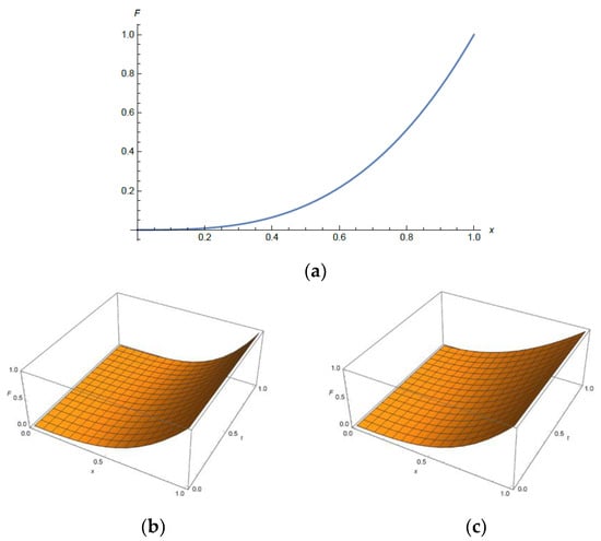
Figure 1.
Elastic force—time—displacement plot for: (a) , (b) , (c) .
3. Model of Oscillator
The model of the oscillator with the time-variable elastic force (1) is
with initial values
where is the small perturbation function.
The procedure for solving (1) is based on the assumption that the approximate solution is the small, perturbed version of the nearly exact solution of the equation with constant parameters [20]. First, the exact solution of the unperturbed, truly nonlinear oscillator in the form of the Ateb function is determined. Then, the approximate solution of (1) is assumed to be the Ateb function with a time-variable amplitude and period. The introduced approximate analytic solution, applied for the perturbed oscillator with a restoring force with a time-variable degree, transforms the Equation (1) into two first-order ones with amplitude and phase functions. After averaging these two equations over the period of the Ateb function, the approximate amplitude and phase functions follow. The approximate solutions are suitable for further discussion.
3.1. Unperturbed Oscillator
For and the degree of nonlinearity is and the Equation (3) transforms into
The equation is the pure nonlinear one. The exact solution of (5) is periodic and has the form of the cosine Ateb function ca [19]
where
A and θ are arbitrary constants, and is the frequency of the ca function. Using the definitions of the derivatives of Ateb functions [19]
the first and the second derivatives of (6) are
where is the sine Ateb function. Substituting (6) and (11) into (5), the frequency of the Ateb function follows as
It is obvious that the frequency of the function depends on the amplitude A of the oscillator and on the constant degree of nonlinearity
3.2. Perturbed Oscillator
Comparing the Equations (3) and (5), it is seen that that (3) is the perturbed version of the Equation (5). As the parameter ε is small, the perturbation is small. Due to the fact that the difference between (3) and (5) is small, the solution of (3) is assumed in the form (6) and (10) with (12), but with time-variable amplitude and phase, i.e.,
where
and
Comparing (14) with the time derivative of (13)
the constraint follows as
where , and
Substituting (13), (14) and the time derivative of (14)
into (3), and after some simplification it is
where .
Introducing the time derivative of (16) and modifying (18) and (21), two first-order differential equations are obtained
Equations (22) and (23) represent the transformed differential Equation (3) with new variables: A and θ.
Finding the solution to the system of two first-order strong nonlinear coupled differential Equations (22) and (23) is not an easy task. It is at this point where averaging of Equations (22) and (23) is introduced. Using the assumption that the Ateb function with the constant degree is periodical, the averaging of (22) and (23) over the period 2, where
and B() is the complete Beta function [], is done. The averaged equations follow as
where . Assuming that the parameter in the periodic function is constant (α = α0 = const.), the values of the averaged functions are
and the averaged equations of motion simplify into
It is obvious that after solving Equation (28) for A, the integration of Equation (29) follows.
4. Special Types of Oscillators and Discussion
4.1. Pure Nonlinear Oscillator
For the pure nonlinear oscillator, the equations of motion (28) and (29) transform into
Integrating (31) for the initial condition , it follows
If the degree of nonlinearity is high and >> 1, the Equation (30) simplifies into
The amplitude of vibration is the solution of the Equation (33). Separating the variables and integrating for the initial conditions and , the amplitude—time function is
where
The frequency function (16) is as
To prove the correctness of the analytic solutions (34) and (36), an example of an oscillator with a high degree of nonlinearity is considered. In Figure 2a, amplitude—time and in Figure 2b, x-t diagrams, obtained numerically, for constant, increasing and decreasing degree of nonlinearity, i.e., , and are plotted. Comparing the results, it is obvious that the analytic solution agrees with the numerical one and that the difference between the numeric and analytic solutions is negligible.
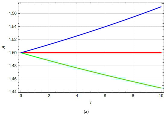
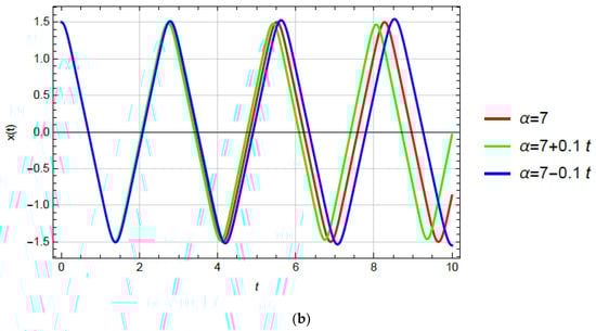
Figure 2.
(a) A-t diagrams, (b) x-t diagrams for: α = 7 (red line), (green line) and (blue line).
4.2. Interaction between the Degree of Nonlinearity and Initial Conditions: Almost Cubic and Linear Oscillators
Relations (34) and (36) depend not only on the degree of nonlinearity but also on the initial amplitude . Thus, for the case when the degree of nonlinearity is increasing over time, and the initial amplitude is the amplitude of vibration is decreasing while the frequency is increasing over time. This result is proved by considering the oscillator with time-degree nonlinearity and initial conditions . The x-t diagrams are plotted in Figure 3.
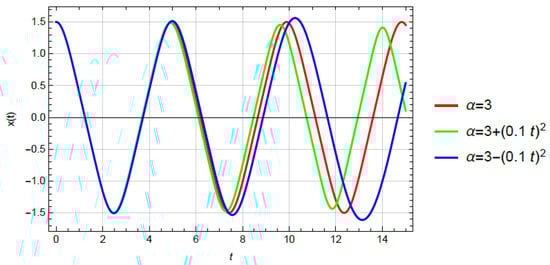
Figure 3.
x-t diagrams for oscillator with constant cubic nonlinearity (red line), increasing degree nonlinearity (green line) and decreasing degree nonlinearity (blue line).
In Figure 3, it is shown that the period of vibration is longer for the oscillator, with time decreasing the degree of nonlinearity compared to the corresponding constant one. In addition, the period of vibration for the oscillator with an increasing degree of nonlinearity is shorter than for the corresponding constant one.
Contrary to the aforementioned results, and according to (34) and (36), it is found that for the case when the degree of nonlinearity increases, and the initial amplitude is the amplitude of vibration increases, and the frequency decreases over time. In Figure 4, the almost linear oscillator with initial conditions is plotted. The degree of nonlinearity is where two types of functions are considered: the linear, i.e., and the quadratic, i.e., . In Figure 4a, it is shown that if the degree of nonlinearity is increasing, the amplitude and period of vibration are higher than for the linear oscillator. The amplitude and the period of vibration increases faster if the degree variation is a linear time function, i.e., for than if it is the quadratic function . If the degree of nonlinearity is decreasing, the amplitude and period of vibration decrease too (Figure 4b). The amplitude and period of vibration of the oscillator with a decreasing degree of nonlinearity are smaller than that of the linear oscillator. The decrease is faster for linear degree variation than for the quadratic one.
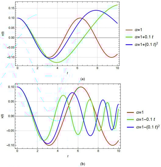
Figure 4.
x-t diagrams for various trends of degree variation: (a) linear and quadratic increasing degree, (b) linear and quadratic decreasing degree.
4.3. Oscillator with Viscous Damping
Substituting the series expansion of the function into (28) and omitting the small terms of the second order, it follows
For the case when the linear viscous damping force acts, the Equation (37) transforms into the Bernoulli equation
where b is the damping coefficient. After integration for the initial amplitude A0 the solution of (38) is
The amplitude variation strongly depends on the time-variable order of nonlinearity but also on the damping coefficient b. Thus, for and the expression (39) is
where the upper sign is for increasing and the lower sign for the decreasing degree . Using (40), the frequency (16) is obtained as
Substituting (40), (41) and = 0 into (13), the x-t relation follows. In Figure 5, the x-t diagrams for various values of damping parameters b are plotted. It is concluded that the damping stops the amplitude increase for (when the degree decreases) and causes amplitude decrease (Figure 5a). For the constant degree of nonlinearity when the amplitude is constant if b = 0 (Figure 5b). However, when damping acts, the amplitude of vibration decreases. In the oscillator with an increasing degree of nonlinearity (Figure 5c), where the amplitude is decreasing over time, the damping causes an additional amplitude decrease.
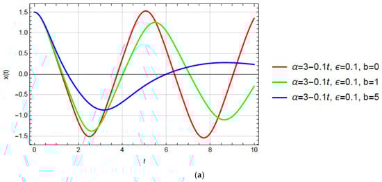
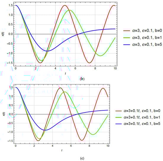
Figure 5.
x-t diagrams for various values of b and various functions of nonlinearity degree variation: (a) ; (b) ; (c) .
5. Vibration of the Fiber-Reinforced Polymer Composite Structure in Aging
Nowadays, in marine, automobile, military and aircraft industries, very often, a special polymer material is applied that is suitable to satisfy the special rough working requirement and also brutal weather conditions. Namely, everyday materials, such as steel or steel-reinforced structures, cannot fulfill the requirements, primarily due to the fact that they are prone to corrosion and weight. To overcome the problem, since 1950, fiber-reinforced polymer (FRP) composites have been widely used in marine environments [21]. Due to their outstanding specific physical/mechanical properties, FRPs have attracted a great amount of interest from the shipbuilding industry [22,23], offshore oil industry [24] and marine infrastructure industry [25], have been used in the recreational craft, workboats and risers for oil exploration and marine renewable energy device components. The application of FRP is for personal boats, the sheathing of wood hulls, submarine sonar domes, pipelines, etc. Usually, three FRPs are applied: glass (fabricated with three types of epoxy materials: polyester, vinyl ester and phenolic resin), basalt and carbon-fiber-reinforced polymers [26], and glass and carbon hybrid composite material. To improve the properties, the nano aluminum embedded glass-fiber-reinforced polymer composites are also produced [27].
However, despite the high strength-to-weight ratio and corrosion properties of the FRP due to exposure to the harsh marine environment (humid, thermal and saline), the mechanical properties vary due to aging over a period of time [28]. The degradation in mechanical properties has become a major issue for the safety and reliability of composite structures [29,30,31]. Chaudhary et al. [32] reported on flexural strength and modulus reduction. Shreepannaga et al. [17] stated that the degradation is up to 20% and more. In the paper of Li et al. [17], the effect of aging in a carbon-reinforced polymer composite structure is presented. The Toray’s Torayca T 700 carbon-fiber-reinforced polymer laminate produced by WuXi RSN New Material Technology Co., Ltd. (Wuxi, China) was considered. Measurements on a sample with the dimensions 60 mm × 13 mm × 3 mm were performed. The results show that the elasticity of the composite is high, and due to aging, it is reduced. The elastic modulus is reduced from the value of 48.32 GPa to 47.16 GPA over 7 months. The tensile strength suffered a reduction from 923.60 MPa to 817.83 MPa. The conclusion was that the future path of research has to be to create an analytical model through which engineers can efficiently compare aged composites with newly formed ones. [17] According to this suggestion, the aim of the research is to give the appropriate mathematical model for the prediction of the change of vibration properties of the structure during aging.
In [29], it is shown that the effect of aging time on the tensile strength is fitted with a decreasing exponential function. Analyzing the measured results, we concluded that the degree of nonlinearity of the composite sample is almost linear. Due to the aforementioned theoretical results, the amplitude (40) and the frequency (41) time functions are considered for . Namely, the amplitude—time function is
and the frequency—time function is
For the linear time function, i.e.,, the simplified expression for amplitude is
In (44), two unknown parameters exist: and ε. Using the initial displacement of 6.728 mm and the failure displacement of 6.297 mm after 7 months of aging, the approximate amplitude function follows as
where ε = 0.02448. Using (45) and (43), the frequency rate is obtained as
where is the initial frequency of the composite. In Table 1, the results of computation according to (45) and (46) are presented. The model gives good agreement of the computed and measured results. In addition, the model gives the prediction of amplitude and frequency of composite due to aging without measuring.

Table 1.
Computed and measured vibration properties of the carbon FRC sample.
6. Conclusions
In this paper, the truly nonlinear oscillator, with a time-variable degree of nonlinearity, is considered. The oscillator is mathematically modeled as a differential equation where the degree of nonlinearity is a time-variable function. The approximate analytic solving procedure had to be developed. The solving method is based on the Ateb function (inverse complete Beta function), which is known to be the solution for the truly nonlinear oscillator. Analyzing the solution of the model, it is concluded:
- For the small initial vibration amplitude in the oscillator with a time-increasing nonlinearity degree, the amplitude and frequency of vibration are decreasing. The increase is faster for the oscillator where the time variation of the degree is linear than where the time variation is quadratic. In contrast, if the initial amplitude is high, the amplitude and frequency of vibration increase with the increase in the degree of nonlinearity.
- An oscillator with a time-variable degree is convenient for the modeling of the aging process in polymer. The amplitude and frequency of vibration for the polymer in aging, computed by using the developed model, are proved to be close to experimentally obtained values.
- The model of an oscillator with nonlinearity of time-variable degree is suitable for predicting oscillatory properties of various structures in aging.
- This model could be generalized to various degradation processes and other processes where the degree of nonlinearity is the slowing-up time-varying function, and it could be used as a guide for engineering applications.
Author Contributions
Methodology, L.C.; Software, M.Z.; Investigation, L.C.; Writing—original draft, L.C.; Visualization, M.Z. All authors have read and agreed to the published version of the manuscript.
Funding
This research received no external funding.
Data Availability Statement
No applicable.
Conflicts of Interest
The authors declare no conflict of interest.
References
- Cveticanin, L.; Cveticanin, D. Vibrations of the Mass Variable Systems. In Chapter in Acoustics and Vibrations of Mechanichal Structures—AVMS-2019; Marinca, V., Herisanu, N., Eds.; Proceedings Physics 251; Springer: Berlin/Heidelberg, Germany, 2021; pp. 25–39. [Google Scholar]
- Kozhushko, A.P.; Kolesnik, I.V.; Lupenko, V.V. Methods of experimental investigation of the determination of dynamic characteristics in the movement of wheeled tractors with units of variable mass. Teh. Inzhenerija 2019, 2, 21–28. [Google Scholar]
- Cveticanin, L. Dynamics of Bodies with Time-Variable Mass; Springer: Berlin/Heidelberg, Germany, 2015. [Google Scholar]
- Cveticanin, L.; Dregelyi, A.; Horvath, R.; Zukovic, M. Dynamics of mass variable rotor and its application in modeling turning operation. Acta Mech. 2021, 232, 1605–1620. [Google Scholar]
- Cao, Z.; Kang, H.; Liu, H.; Duan, L.; Ouyang, Z.; Zhou, Y.; Jiang, G. Modeling and dynamic response of variable mass system of maglev turning electric spindle. Nonlinear Dyn. 2023, 111, 255–275. [Google Scholar]
- Song, K.; Li, X.; Luo, Y.; Huang, J.; Liu, T. Determination of blasting load history in boreholes based on a variable mass thermodynamic system. Eur. J. Environ. Civ. Eng. 2022, 26, 8152–8167. [Google Scholar]
- Chaurasiya, V.; Jain, A.; Singh, J. Numerical study of a non-linear porous sublimation problem with temperature-dependent thermal conductivity and concentration-dependent mass diffusivity. J. Heat. Mass. Transf. 2023, 145, 072701. [Google Scholar]
- Liu, G.; Zheng, D.; Ding, Z.; Yao, H. Experimental study on variable mass negative stiffness dynamic vibration absorber. Zhongguo Jixie Gongcheng/China Mech. Eng. 2018, 29, 538–543. [Google Scholar]
- Huaxia, D.; Guanghui, H.; Jin, Z.; Mingxian, W.; Mengchao, M.; Xiang, Z.; Liandong, Y. Development of a non-piston MR suspension rod for variable mass systems. Smart Mater. Struct. 2018, 27, 1. [Google Scholar]
- Kwiatkowski, R. The concept of vibration damping of the variable mass assembly. In Proceedings of the MATEC Web Conference XXIII Polish-Slovak Scientific Conference on Machine Modelling and Simulations, Rydzyna, Poland, 4–7 September 2018. [Google Scholar]
- Shi, W.; Wang, L.; Lu, Z. Study on self-adjustable tuned mass damper with variable mass. Struct. Control Health Monit. 2018, 25, 16. [Google Scholar]
- Shi, W.; Wang, L.; Lu, Z.; Wang, H. Experimental and numerical study on adaptive passive variable mass tuned mass damper. J. Sound Vib. 2019, 452, 97–111. [Google Scholar]
- Wang, L.; Shi, W.; Zhang, Q.; Zhou, Y. Study on adaptive passive multiple tuned mass damper with variable mass for a large span floor structure. Eng. Struct. 2020, 15, 110010. [Google Scholar]
- Shakib, A.; Ghorbani-Tanha, A.K. An innovative adaptive tuned vibration absorber with variable mass moment of inertia for mitigation of transient response of systems. Struct. Control Health Monit. 2020, 27, 24. [Google Scholar] [CrossRef]
- Chakraborty, S.; Ghosh, A.D.; Chaudhuri, S.R. A novel tuned mass-conical spring system for passive vibration control of a variable mass structure. J. Vib. Control 2022, 28, 1565–1579. [Google Scholar] [CrossRef]
- Zolek-Tryznowska, Z.; Prica, M.; Pavlovic, Z.; Cveticanin, L.; Annusik, T. The influence of ageing on surface free energy of corona treated packaging films. Polym. Test. 2020, 89, 106629. [Google Scholar] [CrossRef]
- Shreepannaga, A.; Vijaya Kini, M.; Pai, D. The ageing effect on static and dynamic mechanical properties of fibre reinforced polymer composites under marine environment—A review. Mater. Today Proc. 2022, 52, 689–696. [Google Scholar] [CrossRef]
- Mickens, R. Truly Nonlinear Oscillations: Harmonic Balance, Parameter Expansions, Iteration, and Averaging Methods; World Scientific: London, UK, 2010. [Google Scholar]
- Cveticanin, L. Strong Nonlinear Oscillators—Analytical Solutions, Mathematical Engineering, 2nd ed.; Springer: Berlin/Heidelberg, Germany, 2018; ISBN 978-3-319-58825-4. [Google Scholar]
- Yu, Y.; Zhou, W.; Zhang, Y.; Bi, Q. Analysis on the motion of nonlinear vibration with fractional order and time variable mass. Appl. Math. Lett. 2022, 124, 107621. [Google Scholar] [CrossRef]
- Nan, J.; Zhi, C.; Meng, J.; Miao, M. Seawater aging effect on fiber-reinforced polymer composites: Mechanical properties, aging mechanism, and life prediction. Text. Res. J. 2023, 93, 3393–3413. [Google Scholar] [CrossRef]
- Morshedsoluk, F.; Khedmati, M.R. Ultimate strength of composite ships’ hull griders in the presence of composite superstructures. Thin-Walled Struct. 2016, 102, 122–138. [Google Scholar] [CrossRef]
- Xie, H.; Ren, H.; Qu, S.; Tang, H. Numerical and experimental study on hydroelasticity in water-entry problem of a composite ship-hull structure. Compos. Struct. 2018, 201, 942–957. [Google Scholar] [CrossRef]
- Felipe, R.C.T.S.; Felipe, R.N.B.; Batista, A.C.M.C.; Aqino, E.M.F. Influence of environmental aging in two polymer-reinforced compositeusing different hybridization methods: Glass/Kevlar fiber hybrid strands and in the weft and warp alternating Kevlar and glass fiber strands. Compos. Part B 2019, 174, 106994. [Google Scholar] [CrossRef]
- Tran, P.; Nguyen, Q.T.; Lau, K.T. Fire performance of polymer-based composites for maritime infrastructure. Compos. B Eng. 2018, 155, 31–48. [Google Scholar] [CrossRef]
- Tan, W.; Na, J.; Ren, J.; Mu, W.; Feng, Y. Aging behavior and failure prediction of interlaminar mechanical properties of carbon fiber reinforced polymer composite at high temperature. Fuhe Cailiao Xuebao/Acta Mater. Compos. Sin. 2020, 37, 859–868. [Google Scholar]
- Nayak, R.K. Influence of seawater aging on mechanical properties of nano-Al2O3 embedded glass fiber reinforced polymer nanocomposites. Constr. Build. Mater. 2019, 221, 12–19. [Google Scholar] [CrossRef]
- Cruz, R.; Correia, L.; Dushimimana, A.; Cabral-Fonseca, S.; Sena-Cruz, J. Durability of epoxy adhesives and carbon fibre reinforced polymer laminates used in strengthening systems: Accelerated ageing versus natural ageing. Materials 2021, 14, 1533. [Google Scholar] [CrossRef] [PubMed]
- Li, H.; Zhang, K.; Fan, X.; Cheng, H.; Xu, G.; Suo, H. Effect of seawater ageing with different temperatures and concentrations on static/dynamic mechanical properties of carbon fiber reinforced polymer composites. Compos. Part B 2019, 173, 106910. [Google Scholar] [CrossRef]
- Hristozov, D.; Wroblewski, L.; Sadeghian, P. Long-term tensile properties of natural fibre-reinforced polymer composites: Comparison of flax and glass fibres. Compos. Part B Eng. 2016, 95, 82–95. [Google Scholar] [CrossRef]
- Fang, Y.; Wang, K.; Hui, D.; Xu, F.; Liu, W.; Yang, S.; Wang, L. Monitoring of seawater immersion degradation in glass fiber reinforced polymer composites using quantum dots. Compos. Part B Eng. 2017, 112, 93–102. [Google Scholar] [CrossRef]
- Chaudhary, V.; Sahu, R.; Manral, A.; Ahmad, F. Comparative study of mechanical properties of dry and water aged jute/flax/epoxy hybrid composite. Mater. Today Proc. 2019, 25, 857–861. [Google Scholar] [CrossRef]
Disclaimer/Publisher’s Note: The statements, opinions and data contained in all publications are solely those of the individual author(s) and contributor(s) and not of MDPI and/or the editor(s). MDPI and/or the editor(s) disclaim responsibility for any injury to people or property resulting from any ideas, methods, instructions or products referred to in the content. |
© 2023 by the authors. Licensee MDPI, Basel, Switzerland. This article is an open access article distributed under the terms and conditions of the Creative Commons Attribution (CC BY) license (https://creativecommons.org/licenses/by/4.0/).