A Novel ANN-Based Radial Basis Function Collocation Method for Solving Elliptic Boundary Value Problems

Abstract

Elliptic boundary value problems (BVPs) are widely used in various scientific and engineering disciplines that involve finding solutions to elliptic partial differential equations subject to certain boundary conditions. This article introduces a novel approach for solving elliptic BVPs using an artificial neural network (ANN)-based radial basis function (RBF) collocation method. In this study, the backpropagation neural network is employed, enabling learning from training data and enhancing accuracy. The training data consist of given boundary data from exact solutions and the radial distances between exterior fictitious sources and boundary points, which are used to construct RBFs, such as multiquadric and inverse multiquadric RBFs. The distinctive feature of this approach is that it avoids the discretization of the governing equation of elliptic BVPs. Consequently, the proposed ANN-based RBF collocation method offers simplicity in solving elliptic BVPs with only given boundary data and RBFs. To validate the model, it is applied to solve two- and three-dimensional elliptic BVPs. The results of the study highlight the effectiveness and efficiency of the proposed method, demonstrating its capability to deliver accurate solutions with minimal data input for solving elliptic BVPs while relying solely on given boundary data and RBFs.

1. Introduction

Elliptic boundary value problems (BVPs) are a class of partial differential equations (PDEs) that arise in various fields of mathematics and physics. Elliptic BVPs can be expressed by mathematical equations that involve partial derivatives of an unknown function with respect to multiple independent variables. They are widely used in various scientific and engineering fields to describe a wide range of physical phenomena. The solution of an elliptic boundary value problem is sought in a domain, and the boundary conditions are imposed on the boundaries of this domain [1,2,3,4].

To solve elliptic BVPs, mesh-free methods have been widely used because of the advantages of the mesh-free characteristics [5,6,7,8]. The radial basis function (RBF) collocation method is a meshless method that uses RBF to approximate the solution of the PDE. It involves placing collocation points in the domain where the solution is sought. The RBFs are centered at these nodes and used to construct the approximation to the unknown function [9,10]. The coefficients of the basis functions are determined by enforcing the PDE at the collocation points, and the solution is obtained by solving a system of linear equations [11,12].

Recently, Ku et al. introduced a novel approach involving simplified RBFs that dispense the need for shape parameters. These RBFs were developed in conjunction with fictitious sources strategically positioned outside the computational domain [13]. The use of fictitious sources in collocation methods has garnered substantial attention due to their exceptional characteristics and their extensive application in the realm of solving PDEs [14,15]. Given the considerable interest surrounding the accuracy of various RBFs when combined with source points in collocation methods for PDE resolution, there exists a strong impetus to explore this topic further. Consequently, this study has chosen to employ the simplified RBFs, which offer a promising avenue for investigation.

The backpropagation neural network is a type of ANN that is widely used for supervised learning tasks [16,17,18,19]. The basic idea behind the backpropagation neural network is to train the network to learn mapping between input data and their corresponding target outputs [20,21,22]. The training process involves adjusting the weights and biases of the network in order to minimize the difference between the predicted outputs and the actual target outputs. This is carried out by using an optimization algorithm that iteratively updates the weights and biases based on the errors between the predicted outputs and the target outputs [23,24,25,26,27].

In this article, we propose a novel ANN-based RBF collocation method for solving elliptic BVPs. We adopt the backpropagation neural network categorized into a type of ANN that is used to learn from the training data and improve its accuracy. The training data consider only the given boundary data from exact solutions and the radial distance of the RBFs between the exterior fictitious sources and boundary points. The RBFs, such as multiquadric (MQ) and inverse multiquadric (IMQ) RBFs, are adopted to construct the neural network for the backpropagation neural network. Unlike the conventional RBF collocation method, the discretization of the governing equation of elliptic BVPs can be avoided. Section 2 outlines the mathematical formulation of the ANN-based RBF collocation method. In Section 3, we delve into a comprehensive analysis of convergence to assess the method’s resilience and efficacy. Section 4 presents a series of inquiries into elliptic BVPs, aiming to illustrate the method’s robustness. Finally, Section 5 summarizes the study’s conclusions.

2. ANN-based RBF Collocation Method

Artificial neural networks (ANNs) are mathematical models inspired by the biological neural networks in the brain, aimed at handling complex information [16,17,18,19]. Comprising numerous interconnected units, ANNs form a complex and non-linear system capable of expressing intricate logic and non-linear relationships.

2.1. Formulation of the Problem

The first step in using ANN-based methods to solve PDEs is to formulate the problem as an optimization task. In the context of solving PDEs, the goal is to find the parameters of the neural network (weights and biases) that minimize the error between the network’s predictions and the actual solutions of the PDE at different points in the domain. For elliptic BVPs, the unknown function depends on multiple independent variables, and the highest-order derivatives involved are of second order. The general form of an elliptic BVP is typically represented as:

$${\nabla }^{2}u(x)+V\cdot \nabla u(x)+F(x)u(x)=f(x),$$

(1)

$$u(x)=g(x) \mathrm{on} \partial \mathsf{\Omega },$$

(2)

where $\nabla$ denotes the operator of gradient; x denotes the coordinate, described as $x=(x,y,z)$; $u(x)$ is the variable of interest; V is the velocity, defined as $V=(V_x,V_y,V_z)$; $F(x)$ and $f(x)$ denote the provided function; $g(x)$ denotes the boundary conditions; and $\mathsf{\Omega }$ is the domain with the boundary $\partial \mathsf{\Omega }$.

2.2. Preparation of the Data

Data preparation is a crucial step when using the ANN-based RBF collocation method for solving elliptic BVPs. It involves collecting and organizing the input and output pairs that are used to train the neural network. In this study, we proposed an ANN-based RBF collocation method for solving elliptic BVPs. A simplified version of RBFs was introduced by Ku et al. by eliminating the shape parameter and utilizing fictitious sources located outside the domain [13,14,15]. Three simplified RBFs, specifically MQ, IMQ, and Gaussian, without the inclusion of the shape parameter, c, are introduced for the resolution of elliptic BVPs, as follows.

$$\mathrm{Simplified} \mathrm{MQ} \mathrm{RBF}: \phi \left(r_i\right)=r_i,$$

(3)

$$\mathrm{Simplified} \mathrm{IMQ} \mathrm{RBF}: \phi \left(r_i\right)=\frac{1}{r_i},$$

(4)

$$\mathrm{Simplified} \mathrm{Gaussian} \mathrm{RBF}: \phi (r_i)=e^{-{\left(\frac{r_i}{R}\right)}^2},$$

(5)

where $\phi \left(r_i\right)$ is the simplified RBF; $r_i$ denotes the radial distance; $r_i=\left|x-x_i^s\right|$, at the i^th source point; $x_i^s$ denotes the i^th source point, defined as $x_i^s=(x_i^s,y_i^s,z_i^s)$; and R denotes the parameter corresponding to the maximum radial distance. The range of subscript i is defined as i = 1, 2, ..., and similarly, the range of superscript s is defined as s = 1, 2, .... The corresponding boundary data value using analytical solutions or simulation data are utilized as output. For each selected collocation point, the corresponding solution value $u_i$ is evaluated using analytical solutions. The analytical solutions employed are expressed in functional form and are referenced from the relevant literature sources. To calculate the field solution within the computational domain for any selected collocation point, one simply needs to provide the coordinates of that point within the domain and then compute the solution values by substituting these coordinates into the corresponding analytical solutions. These pairs, including the RBF $\phi \left(r_i\right)$ and $u_i$, form the input–output training data for the ANN-based RBF collocation method.

Once the RBF interpolation functions are selected, these functions could be used to generate training data for the ANN-based RBF collocation method. The RBFs $\phi \left(r_i\right)$ are constituted as training data for the ANN-based RBF. The simplification of the RBFs involves removing the shape parameter from the original RBF formulation, as shown in

Table 1. The simplified RBFs [14].

The RBF Type	Original	Simplified
Gaussian	$\phi (r_i)=e^{-{\left(\frac{r_i}{c}\right)}^2}$	$\phi (r_i)=e^{-{\left(\frac{r_i}{R}\right)}^2}$
Multiquadric (MQ)	$\phi \left(r_i\right)=\sqrt{r_i{}^2+c^2}$	$\phi \left(r_i\right)=r_i$
Inverse multiquadric (IMQ)	$\phi \left(r_i\right)=\frac{1}{\sqrt{r_i{}^2+c^2}}$	$\phi \left(r_i\right)=\frac{1}{r_i}$

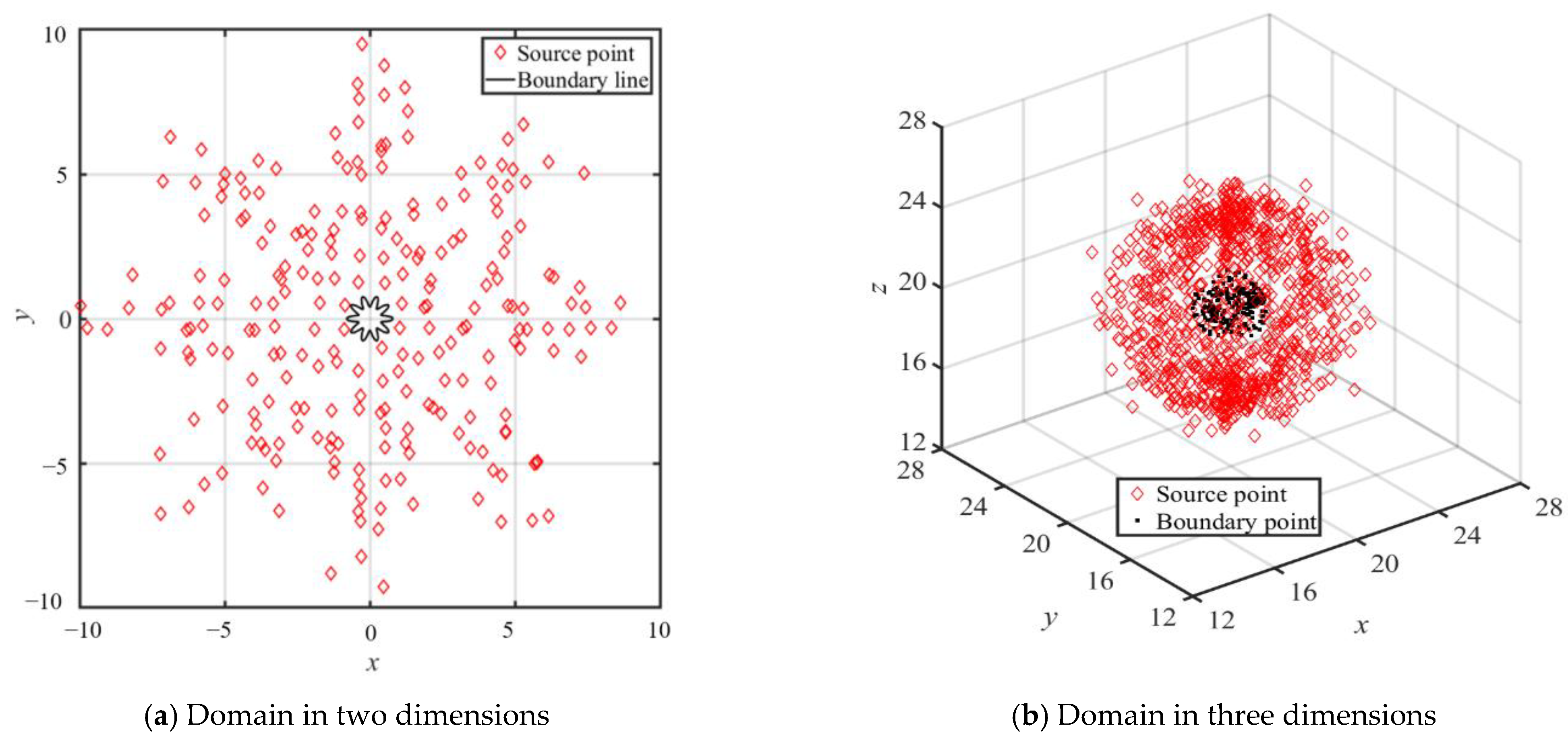
Notation: c denotes shape parameter.

. In the simplified RBF collocation method, only the boundary and source points are positioned, as illustrated in Figure 1a, for two-dimensional domains and for three-dimensional domains, as shown in Figure 1b. Significantly, the employment of simplified RBFs in conjunction with exterior fictitious sources substantially enhances accuracy, particularly when tackling the Laplace equation. Moreover, these simplified RBFs offer the advantage of simplifying the resolution of elliptic BVPs without the necessity of determining an optimal shape parameter [13,14,15]. Consequently, these simplified RBFs are adopted in the present ANN-based RBF collocation method.

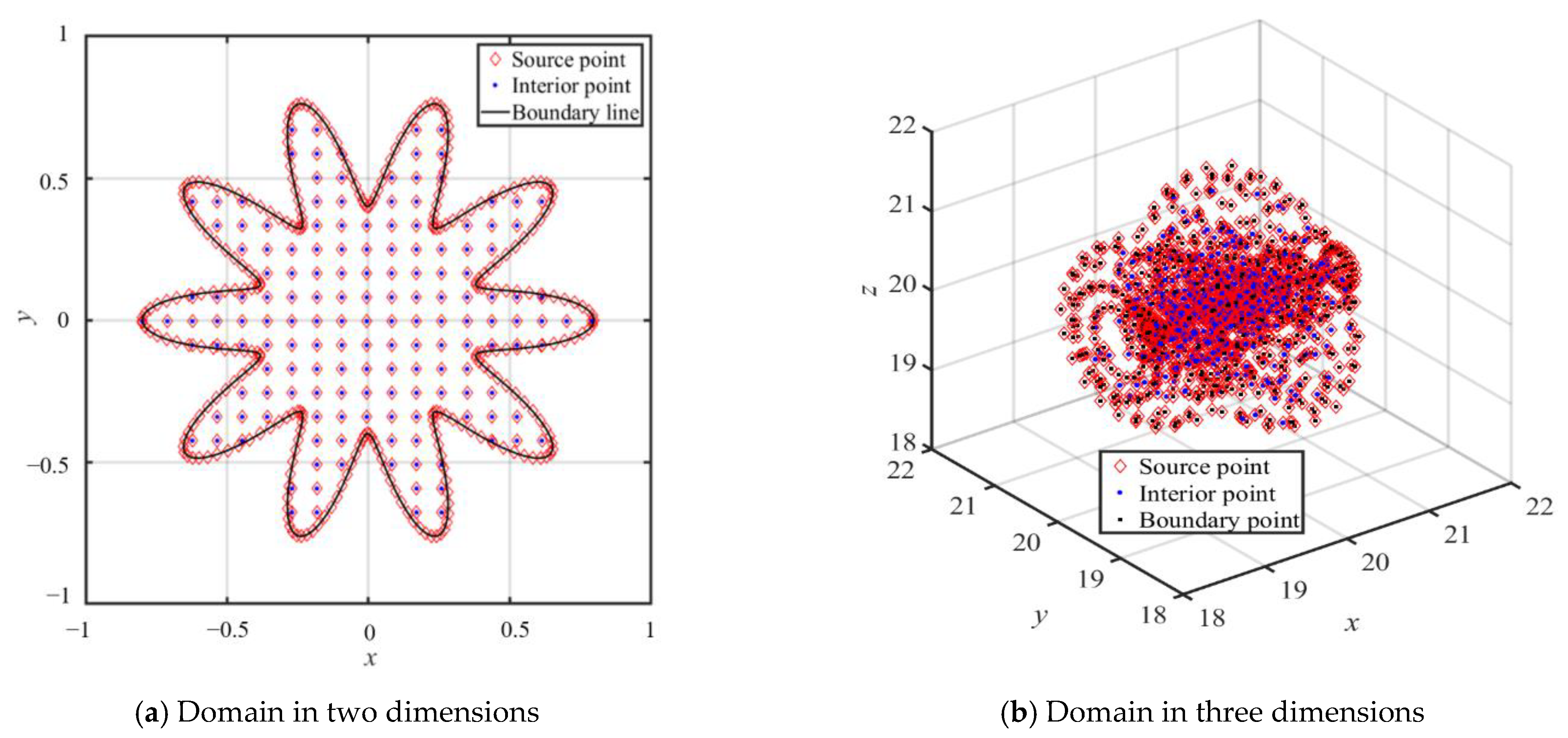
Comparing to the conventional RBF collocation method, the interior, center, and boundary points are positioned such that the interior and source points coincide at the same locations, as illustrated in Figure 2a for two-dimensional domains and Figure 2b for three-dimensional domains. By comparing the traditional RBF collocation method and the proposed ANN-based RBF collocation method, we aim to gain insights into their strengths and limitations in solving elliptic BVPs efficiently and accurately. One of the key advantages of this approach is its ability to avoid the discretization of the governing equation of elliptic BVPs. As a result, this method offers simplicity in solving elliptic BVPs with only given boundary data and RBFs.

2.3. Construction of the Neural Network Architecture

The construction of the neural network architecture involves designing an appropriate neural network architecture that can approximate the solution of the given PDE. This typically involves defining the input layer to represent the spatial coordinates of the problem, hidden layers that perform computations, and an output layer that provides the predicted solution.

To solve an elliptic BVP as Equation (1), the process begins with the generation of weights. These weights are combined linearly with the inputs and the bias term. Assuming a hidden layer with N neurons, the computation for each neuron j in the hidden layer can be described as follows:

$$H_j={\displaystyle \sum _{i=1}^p[w_{ij}\phi (r_i\left)\right]}+b_j,$$

(6)

where $H_j$ denotes the weighted sum at neuron j in the hidden layer; $w_{ij}$ denotes the weight from the input unit $\phi \left(r_i\right)$ from the input layer to neuron j in the hidden layer; $\phi \left(r_i\right)$ denotes the RBF which is the input value; $b_j$ denotes the bias term for neuron j in the hidden layer; and p denotes the total number of inputs from the input layer. This weighted sum serves as the input to the activation function for the neuron. The output of the activation function represents the neuron’s final activation value. The weighted sum is the result of combining Inputs with their respective weights and biases for a single neuron, while the hidden layer consists of multiple neurons, each with its own weighted sum calculation and activation.

Subsequently, the combination is utilized to compute the hidden layer, as outlined in Equation (6), in the above manner. After inputting the activations from the first hidden layer into a specific neuron j in the subsequent hidden layers of a neural network, the data undergo processing to generate the output layer described as follows:

$$H_{ij}={\displaystyle \sum _{j=1}^q{\displaystyle \sum _{i=1}^p{v}_{ij}f(H_j)}+b_{ij}},$$

(7)

where $H_{ij}$ denotes the weighted sum at neuron i in the j^th hidden layer; $v_{ij}$ denotes the weight associated with the activation function from the hidden layer to neuron i in the j^th hidden layer; $b_{ij}$ denotes the bias term for neuron i in the j^th hidden layer; q denotes the number of neurons in each hidden layer; and f denotes the activation function described as follows

$$f(H_j)=\frac{e^{H_j}-e^{-H_j}}{e^{H_j}+e^{-H_j}}.$$

(8)

Activation functions are widely employed to facilitate diverse computations between layers. Common activation functions include sigmoid or logistic, hyperbolic tangent (tanh), rectified linear unit (ReLU), and Leaky ReLU [21]. In this study, the hyperbolic tangent function (tanh) is chosen due to its demonstrated ability to yield superior results compared to alternative activation functions.

The objective of this study is to acquire an approximate solution of elliptic BVP, denoted by the following expression:

$$u_{net}={\displaystyle \sum _{j=1}^q{m}_{j}f(H_{ij})},$$

(9)

where $u_{net}$ denotes the approximate solution and $m_j$ denotes the weights of the output layers. To regulate the accuracy of the approximate solution, a comparison is made between the solution and the right-hand side of the given elliptic BVP as shown in Equation (1). This comparison necessitates the partial differentiation of the $u_{net}$ model, as outlined in the following manner:

$$\frac{{\partial }^k{u}_{net}}{\partial x^k}={\displaystyle \sum _{j=1}^q{m}_j\frac{{\partial }^{k}f(H_{ij})}{\partial x^k}},$$

(10)

$$\frac{{\partial }^k{u}_{net}}{\partial y^k}={\displaystyle \sum _{j=1}^q{m}_j\frac{{\partial }^{k}f(H_{ij})}{\partial y^k}},$$

(11)

$$\frac{{\partial }^k{u}_{net}}{\partial z^k}={\displaystyle \sum _{j=1}^q{m}_j\frac{{\partial }^{k}f(H_{ij})}{\partial z^k}},$$

(12)

where k = 1, 2.

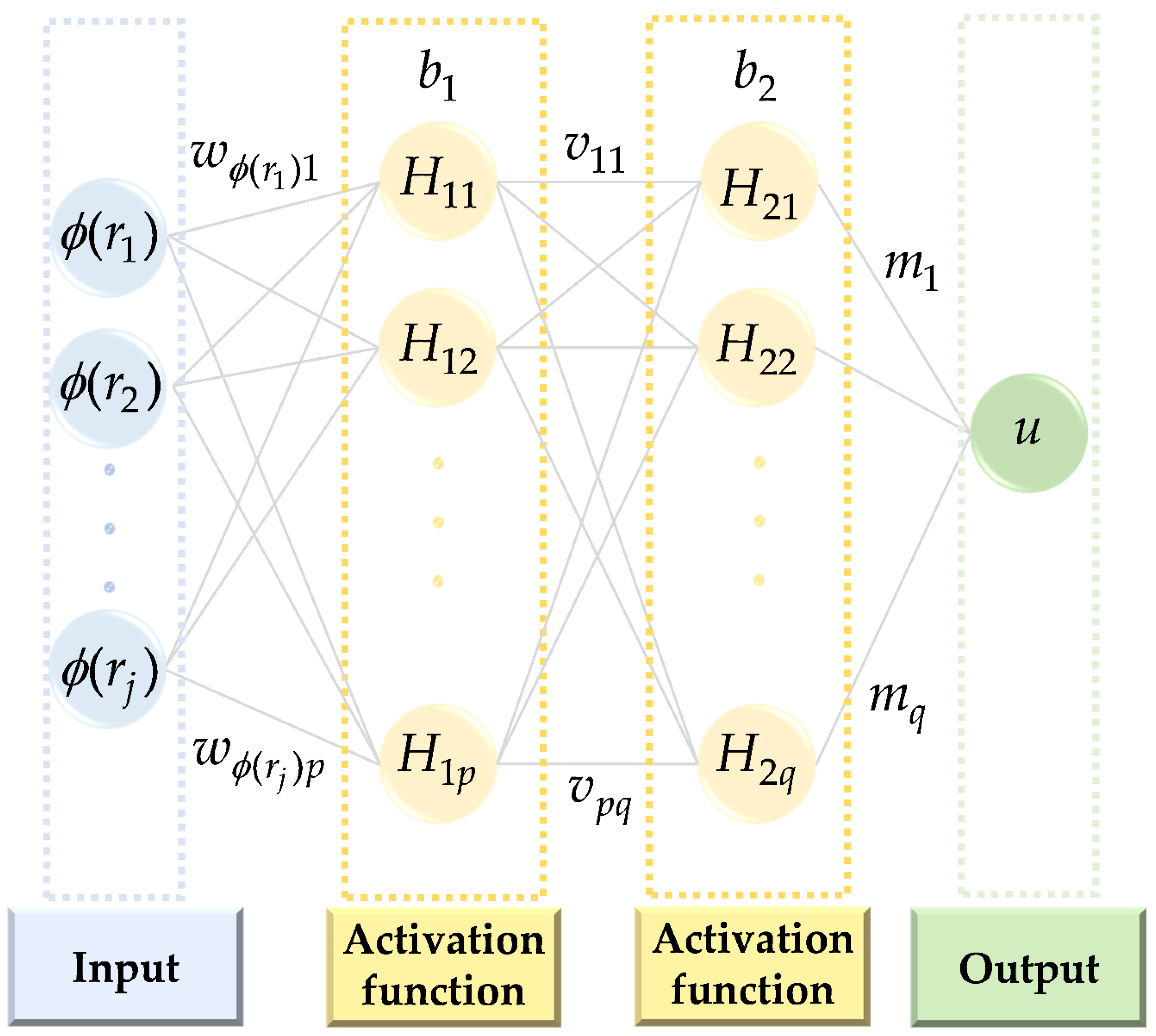
Figure 3 illustrates the architecture of an ANN-based RBF neural network, with the input feeding into the first neural network unit. The connections between nodes represent weighted values for signal transmission. Signal processing is simulated in the neural network by assigning a weight to each input before it enters the neural unit. These weights collectively form the weight vector. Each node in the network corresponds to a specific output function known as an activation function. The final output of the network is influenced by its structural arrangement, connectivity, weights, and activation functions.

As illustrated in Figure 3, the connections between each pair of nodes in the network correspond to weighted values, which determine the signal transmission through the connections. The neural network operates by simulating signal processing in this manner. Prior to entering the neural unit, each input quantity is associated with a weight. Each node in the network is associated with a specific output function, referred to as an activation function. The network’s output is influenced by several factors, including the network’s structure, connectivity, weights, and activation functions.

In this study, the backpropagation neural network is employed in the ANN-based RBF neural network, enabling learning from training data and enhancing accuracy. The training data consist of given boundary data from exact solutions and the radial distances between exterior fictitious sources and boundary points, which are used to construct RBFs, such as MQ, IMQ, and Gaussian RBFs. The distinctive feature of this approach is that it avoids the discretization of the governing equation of elliptic BVPs. Consequently, the proposed ANN-based RBF collocation method offers simplicity in solving elliptic BVPs with only given boundary data and RBFs.

2.4. Measurement the Loss Function

After the construction of the neural network, the loss function is then utilized to measure the difference between the network’s predicted solution and the actual solution of the PDE [28]. The mean-squared error loss is adopted for the training of the network’s weights through error backpropagation as follows:

$$L=\frac{1}{M}{\displaystyle \sum _{i=1}^M{(u_{net,i}-u_i)}^2},$$

(13)

where M denotes the number of data points in the dataset and $u_i$ denotes the target solutions. The above loss function captures the difference between the predicted solution and the actual solution at each data point. In this study, the Levenberg–Marquardt algorithm is used as an optimizer to minimize the loss function. The goal of training the neural network using the Levenberg –Marquardt algorithm is to minimize this loss function across the entire dataset. By updating the network’s weights and biases iteratively, the algorithm aims to find the combination of parameters that leads to the lowest possible value of the loss function. This iterative process precisely adjusts the network’s parameters, resulting in predictions that exhibit a significantly improved alignment with the true solutions of the elliptic BVPs.

2.5. Training Process

During each iteration, it updates the weights and biases to reduce the error. The update rule for the k-th iteration is as follows:

$$\Delta w=-{(J+{\lambda }^{k}H)}^{-1}\nabla L^k,$$

(14)

where w denotes the weights; J denotes the Jacobian matrix, representing the gradients of the predicted outputs with respect to the weights and biases; H denotes the Hessian matrix, which accounts for the curvature of the loss function; $\lambda$ denotes the damping parameter, which balances between the Levenberg and Marquardt steps; and $\nabla L^k$ denotes the gradient of the loss function at the k^th iteration.

The Levenberg–Marquardt algorithm combines gradient information with the Hessian matrix to update the network’s parameters. It dynamically adjusts the update step size using a damping parameter enabling the algorithm to balance convergence speed and stability during the optimization process. This regularization term ensures that the optimization remains stable and avoids overshooting the optimal solution.

Based on the loss function, it serves as the guiding metric for the Levenberg–Marquardt algorithm to iteratively adjust the neural network’s parameters in a way that minimizes the discrepancy between the predicted and actual solutions of the elliptic BVPs. This optimization process leads to a neural network that approximates the elliptic BVPs solution with greater accuracy. The damping parameter helps control the step size of updates. A larger value of the damping parameter may ensure stability, while smaller values of the damping parameter aid in faster convergence. The algorithm iteratively updates the weights and biases using the Levenberg–Marquardt formula and recalculates the loss. The process continues until a stopping criterion is met, such as reaching a certain number of iterations or achieving a sufficiently small change in the error.

2.6. Prediction

After convergence, the neural network’s weights and biases represent the approximate solution to the elliptic BVPs that minimizes the error between the predicted and actual solutions. The Levenberg–Marquardt algorithm, when combined with neural networks, facilitates solving elliptic BVPs by iteratively adjusting the network’s parameters to minimize the error between the network’s predictions and the actual solutions of the elliptic BVPs. This optimization process enables the network to learn and approximate the complex relationships within the elliptic BVPs, leading to an accurate solution representation.

After training, the trained network is used to predict solutions at any point within the problem domain. Input the relevant values into the network, and it could provide an approximation of u based on what it has learned.

2.7. Accuracy and Validation

To assess the effectiveness and precision of the proposed method, this study utilizes the root-mean-square error (RMSE) and the maximum absolute error (MAE) as evaluation metrics.

$$\mathrm{RMSE}=\sqrt{{\displaystyle \sum _{i=1}^{N_T}{\left|u_A\left(x_i\right)-u_N\left(x_i\right)\right|}^2/N_T}},$$

(15)

$$\mathrm{MAE}=\left|u_A\left(x_i\right)-u_N\left(x_i\right)\right|,$$

(16)

where $N_T$ is the number of points used for validation, $u_A\left(x_i\right)$ is the analytical solution, and $u_N\left(x_i\right)$ is numerical solutions.

The merits of the presented ANN-based RBF collocation technique for the resolution of elliptic BVPs encompass the notable attributes of domain flexibility and proficiency in addressing high-dimensional challenges. Capitalizing on the intrinsic meshless nature, the proposed methodology demonstrates its efficacy by obviating the reliance on predefined grids. This characteristic renders it particularly well suited for intricate domains characterized by irregularity and intricate geometries. Furthermore, the devised ANN-based approach exhibits a commendable capability to effectively manage problems characterized by a multitude of input dimensions.

Furthermore, a significant advantage lies in its capacity to perform robust interpolation within the training data range and extend its capabilities through extrapolation beyond the confines of the training data. This adaptability contributes to its versatility and wide-ranging applicability. In essence, the utilization of meshless methods underpinned by ANNs involves the training of neural network models to directly approximate solutions for continuous problems, circumventing the reliance on grid-based discretization strategies.

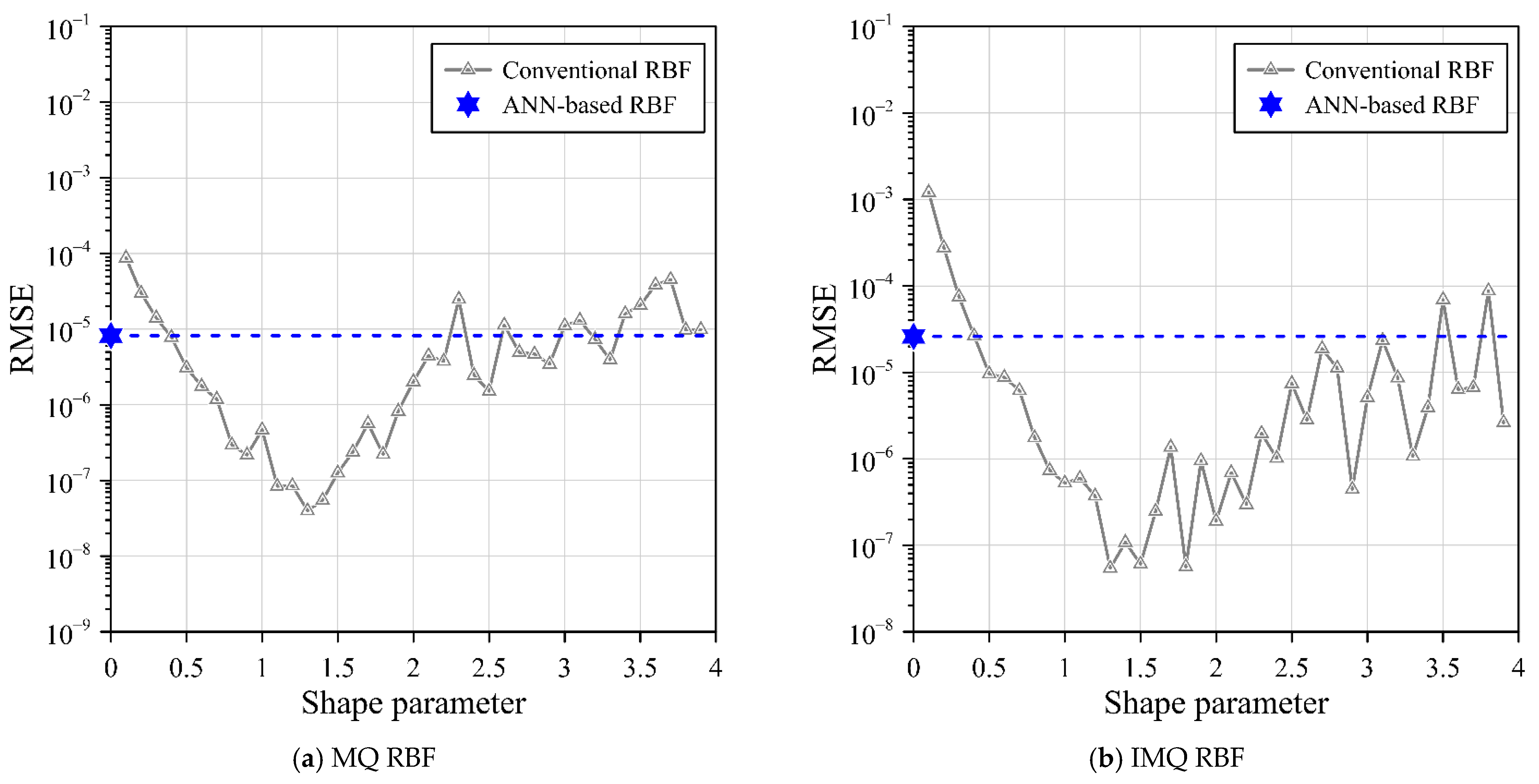
3. Validation Example

To evaluate accuracy, comparative analysis of three distinct RBF collocation methods for solving elliptic BVPs is conducted. The two-dimensional Laplace equation is expressed as Equation (1), where $A=B=f(x)=0$. The boundary of the computational domain is specified as follows:

$$\begin{array}{l}\partial \mathsf{\Omega }=\left\{(x,y)|x=\rho (\theta )\cos \theta , y=\rho (\theta )\sin \theta \right\},\\ \rho (\theta )=0.4[e^{\sin (\theta )}{\sin }^4(4\theta )+e^{\cos (\theta )}{\cos }^4(4\theta )], 0\le \theta \le 2\pi \end{array}.$$

(17)

The analytical solution [13] is adopted for boundary conditions as follows:

$$u(x,y)=\cos (x)\cosh (y)+\sin (x)\sinh (y).$$

(18)

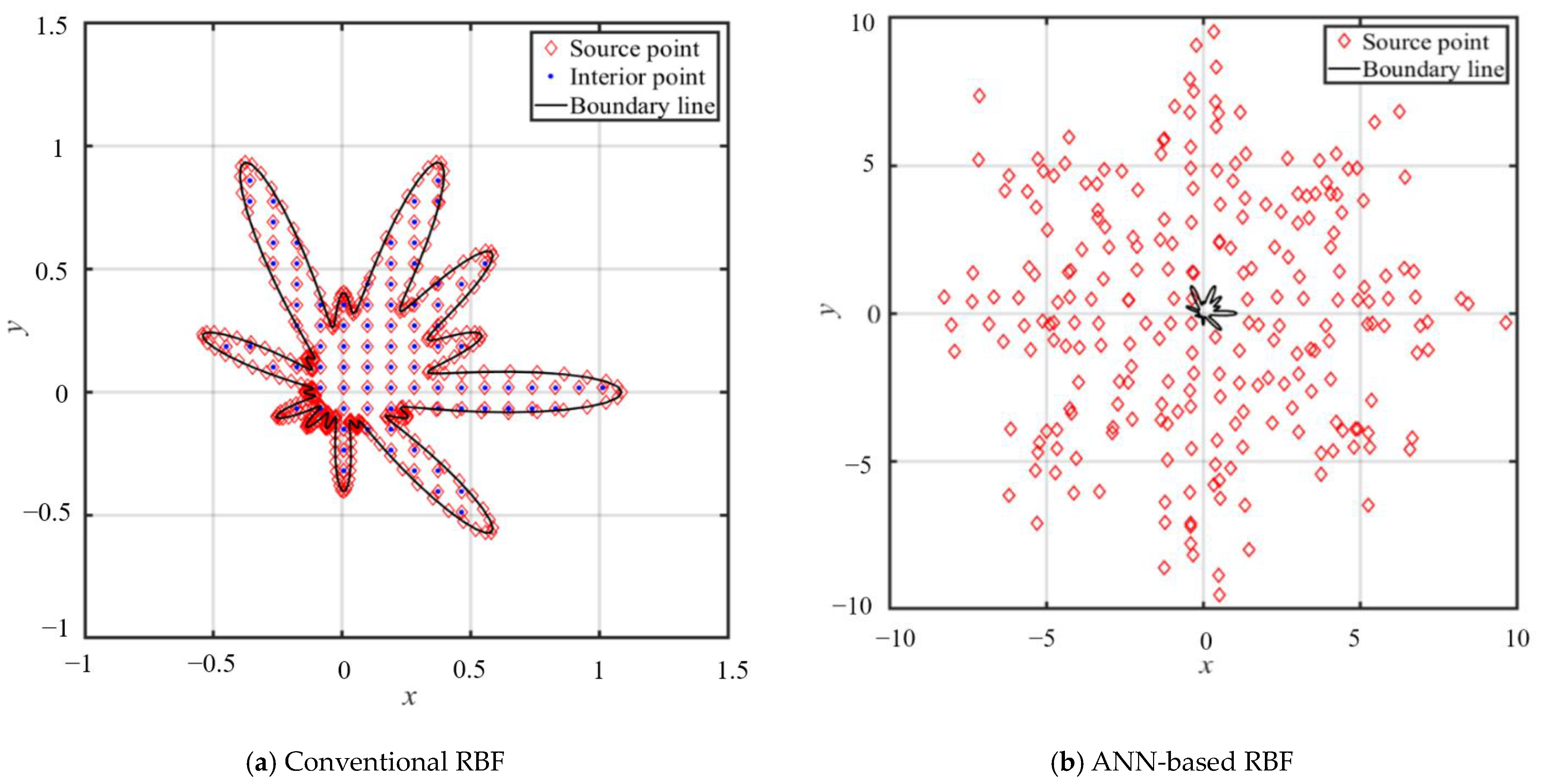
In this study, we employ the conventional and simplified RBFs coupled with the MQ, IMQ, and Gaussian collocation methods to address the problem. In the conventional RBF collocation method, source points are distributed throughout the domain, as shown in Figure 4a. The configuration of interior, source, and boundary points ensures that the location of the interior points align perfectly with those of the source points. In the conventional RBF approach, a combined total of 342 inner points, 238 source points, and 120 boundary points are incorporated.

Alternatively, the ANN-based RBF collocation method adopts a different approach. We only need to position the boundary and source points, as depicted in Figure 4b. The source points are treated as fictitious centers distributed randomly throughout the exterior domain, as illustrated in Figure 4b. The use of exterior source points is governed by following parametric equations, allowing for greater flexibility and versatility in addressing a wide range of practical problems. The positions of the exterior source points are determined as follows:

$$\partial {\mathsf{\Omega }}^s=\left\{(x_j^s,y_j^s)|x_j^s=\eta {\rho }_j^s({\theta }_j^s)\cos {\theta }_j^s, y_j^s=\eta {\rho }_j^s({\theta }_j^s)\sin {\theta }_j^s\right\},$$

(19)

where $\eta$ represents the dilation factor, and ${\rho }_j^s$ and ${\theta }_j^s$ represents the radius and angle of the source point, respectively, defined as ${\rho }_j^s({\theta }_j^s)=2\times [\sqrt[1/3]{\cos (10{\theta }_j^s)+\sqrt{2-{\sin }^2(10{\theta }_j^s)}}], 0\le {\theta }_j^s\le 2\pi$. $\eta$ is 7. A total of 238 source points and 120 boundary points are used in the ANN-based RBF.

In the ANN-based RBF, the dataset division into training, testing, and validation subsets in a proportion of 70% for training, 15% for testing, and 15% for validation. The proposed ANN-based RBF architecture encompassed three hidden layers. The Levenberg–Marquardt optimization technique was utilized for updating weight and bias values during network training, owing to its efficacy. Notably, the Levenberg–Marquardt function is recognized for its speed and minimal memory requirements compared to other algorithms. During the training process, several parameters governed the optimization. Training occurred over a maximum of 1000 epochs. The performance goal was set to 0, indicating a desire for optimal performance. A threshold of six validation failures was set as the maximum allowable value. The minimum acceptable performance gradient was established at 10⁻⁷. The initial value of the damping parameter (mu) was initialized at 10⁻³. A decrease factor of 0.1 and an increase factor of 10 were employed for updating mu. Finally, the upper bound for mu was capped at 10¹⁰.

The model’s performance was assessed using the mean-squared error as an evaluation metric. The validation results indicate that the mean-squared error achieved by the ANN-based RBF utilizing MQ, IMQ, and Gaussian functions was 10⁻⁹, 10⁻¹⁰, and 10⁻⁷, respectively, by the 1000th epoch. The training data’s correlation coefficient remained consistently at 1 for the training, validation, and testing datasets. This correlation coefficient of 1 signifies a robust alignment between the exact solution and the predictions produced by the proposed model. This strong correlation is visually demonstrated in Figure 5. These findings collectively confirm the effectiveness of the proposed ANN-based RBF in accurately addressing the Laplace equation within a two-dimensional context.

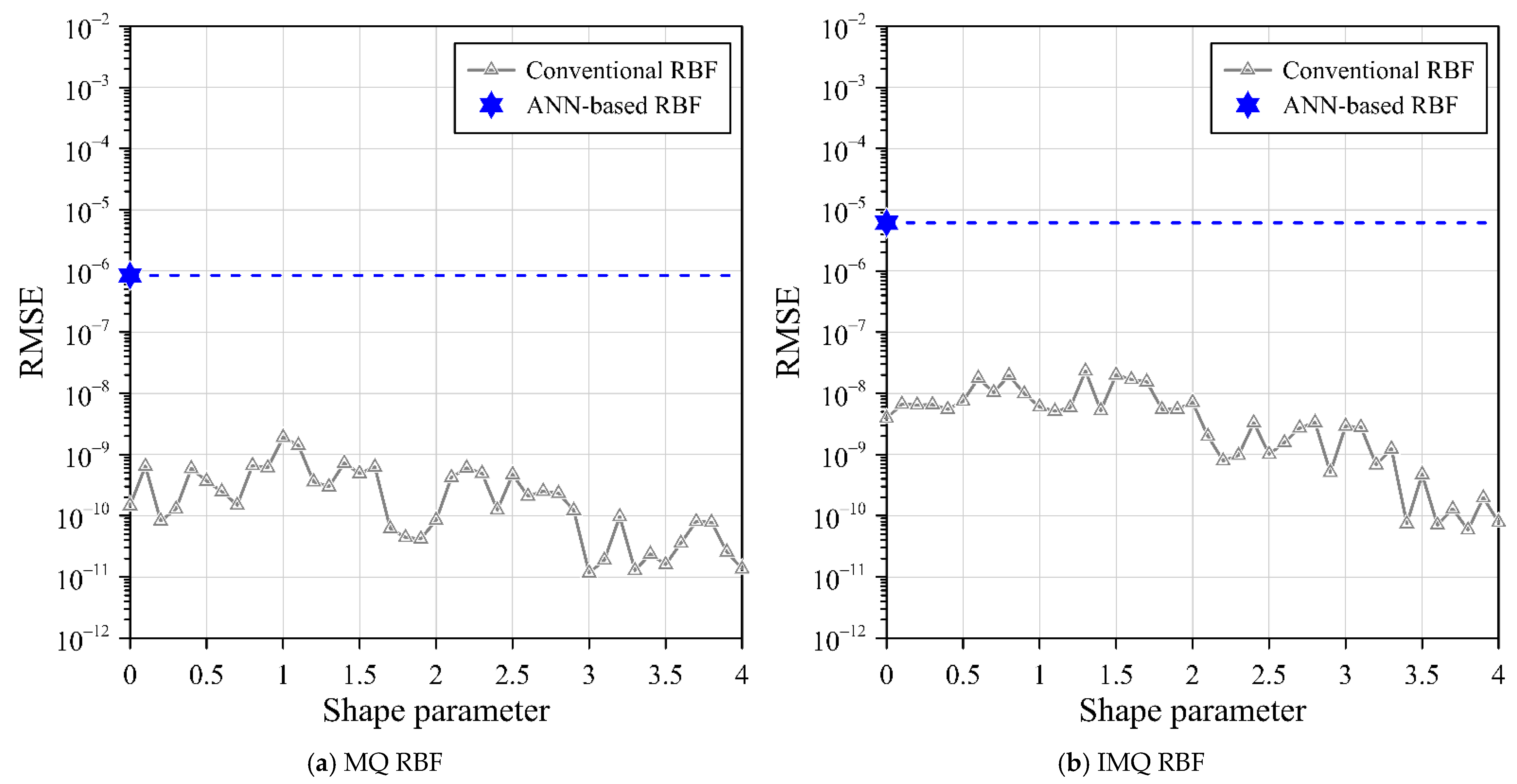
To facilitate comparison, the RMSE and MAE metrics are employed to assess the accuracy of the computed outcomes. Subsequently, a thorough analysis of accuracy among different RBFs is conducted. The outcomes of this analysis are summarized in

Table 2. Comparative results for the validation example.

	RMSE		MAE
	Conventional RBF	ANN-Based RBF	Conventional RBF	ANN-Based RBF
MQ	1.30 × 10–8 (c = 1.30)	8.21 × 10–6 (without c)	1.16 × 10–4 (c = 1.30)	1.52 × 10–4 (without c)
IMQ	1.81 × 10–8 (c = 1.25)	2.60 × 10–5 (without c)	1.89 × 10–4 (c = 1.25)	8.80 × 10–5 (without c)
Gaussian	1.53 × 10–7 (c = 0.40)	9.79 × 10–3 (without c)	5.32 × 10–4 (c = 0.40)	1.17 × 10–2 (without c)

, which contrasts the RMSE values attained through both conventional RBF and the proposed ANN-based RBF approaches. As listed in Table 2, all variations of the ANN-based RBF method—utilizing MQ, IMQ, and Gaussian RBFs in conjunction with exterior fictitious sources—yield notably precise outcomes. Specifically, the proposed ANN-based RBF employing MQ, IMQ, and Gaussian RBFs, while employing exterior source points, demonstrate commendable accuracy, boasting RMSE values to the order of 10⁻⁶, 10⁻⁵, and 10⁻³, respectively.

The outcomes reveal that the ANN-based RBF collocation method with exterior fictitious sources can effectively address this two-dimensional Laplace problem with remarkable accuracy, as depicted in Figure 6. Most importantly, the distinctive feature of the proposed ANN-based RBF is that it avoids the discretization of the governing equation. Consequently, the proposed ANN-based RBF collocation method offers simplicity in solving elliptic BVPs with only given boundary data and RBFs.

4. Application Examples

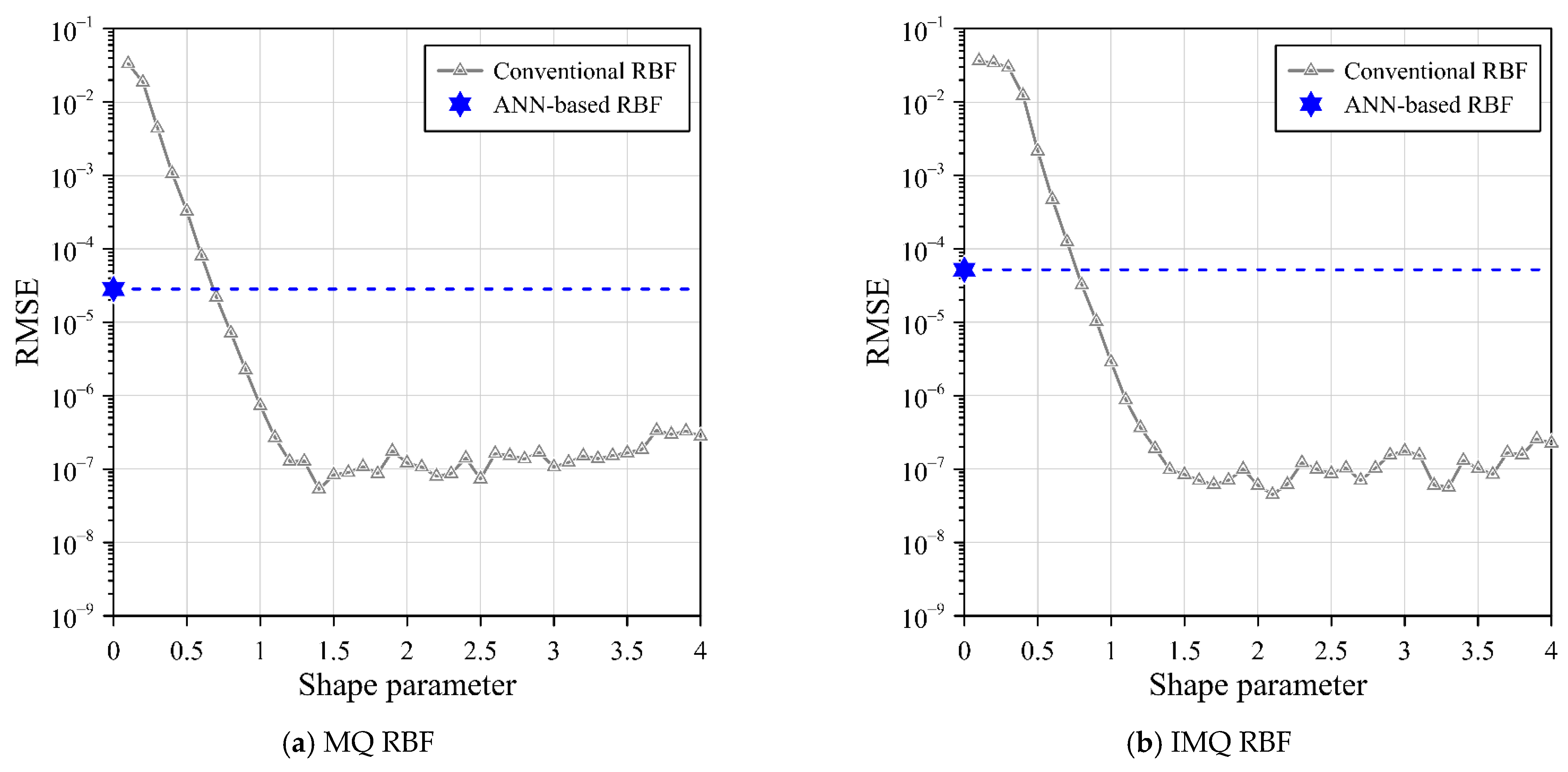
4.1. Example 1: Two-Dimensional Poisson Equation

The two-dimensional Poisson equation is expressed in Equation (1), in which $f(x)=-\left[x\cos (y)+y\sin (x)\right]$, and $A=B=0$. The boundary is described as follows:

$$\begin{array}{l}\partial \mathsf{\Omega }=\left\{(x,y)|x=\rho (\theta )\cos \theta , y=\rho (\theta )\sin \theta \right\},\\ \rho (\theta )=0.4[e^{\sin (\theta )}{\sin }^2(3\theta )+e^{\cos (\theta )}{\cos }^2(3\theta )], 0\le \theta \le 2\pi \end{array}.$$

(20)

The boundary condition is enforced by employing the analytical solution [29] as follows:

$$u(x,y)=x\cos (y)+y\sin (x).$$

(21)

In this research, we apply both the ANN-based RBF and traditional RBF approaches in conjunction with the MQ, IMQ, and Gaussian collocation techniques to tackle the issue at hand. In the conventional RBF collocation method, source points are scattered across the domain, as illustrated in Figure 7a. The organization of the source, interior, and boundary points ensures that the positions of the interior points align precisely with those of the source points. In this configuration, we employ a total of 120 boundary points, 120 source points, and 120 interior points.

On the other hand, the ANN-based RBF collocation method follows a distinct approach. Here, we focus solely on positioning the boundary and source points, as shown in Figure 7b. The source points are distributed randomly in the exterior domain, as illustrated in Figure 7b. The placement of these exterior source points is determined by parametric equations, providing enhanced flexibility and adaptability for addressing a wide array of real-world problems. The precise location of these exterior source points is defined by Equation (19), resulting in a configuration consisting of 120 source points and 120 boundary points.

The dataset for the ANN-based RBF is partitioned into distinct subsets for training, testing, and validation. These subsets are allocated in proportions of 70%, 15%, and 15%, respectively. The ANN-based RBF architecture comprised three hidden layers. The training process was facilitated by the Levenberg–Marquardt algorithm, and the evaluation of model performance was executed through the calculation of the mean-squared error. The results unveiled that the mean-squared error of validation performance reached 10⁻⁴ by the 91st epoch. Moreover, the correlation coefficients for the training, validation, and testing datasets stood uniformly at 0.99. This remarkably high correlation coefficient underscores a robust correspondence between the exact solution and the predictions of the proposed model. Conclusively, these outcomes affirm the efficacy of the proposed ANN-based RBF in effectively tackling the two-dimensional Poisson equation.

For the purpose of comparison, the RMSE and MAE metrics are employed to assess the precision of the computed outcomes. Comparisons are detailed in

Table 3. Results for the two-dimensional Poisson equation.

	RMSE		MAE
	Conventional RBF	ANN-Based RBF	Conventional RBF	ANN-Based RBF
MQ	5.31 × 10–8 (c = 1.40)	2.83 × 10–5 (without c)	1.17 × 10–5 (c = 1.40)	6.28 × 10–5 (without c)
IMQ	4.50 × 10–8 (c = 2.10)	5.21 × 10–5 (without c)	7.93 × 10–6 (c = 2.10)	8.80 × 10–5 (without c)
Gaussian	3.35 × 10–8 (c = 0.40)	4.28 × 10–2 (without c)	3.92 × 10–5 (c = 0.40)	2.66 × 10–1 (without c)

, which presents a contrast between the RMSE values obtained from conventional RBF and the proposed ANN-based RBF. All variations of the ANN-based RBF approach, encompassing MQ, IMQ, and Gaussian RBFs while employing exterior source points, yield outcomes of notable accuracy. To elaborate further, the ANN-based RBF collocation method with simplified MQ, IMQ, and Gaussian RBFs, when integrated with exterior fictitious sources, offers precise results, characterized by RMSE values to the order of 10⁻⁵, 10⁻⁵, and 10⁻², respectively. These outcomes collectively underscore the efficacy of employing the ANN-based RBF, complemented by exterior source points, in achieving accurate solutions for the two-dimensional Poisson problem. This is visibly corroborated by the results illustrated in Figure 8.

4.2. Example 2: Two-Dimensional Modified Helmholtz Equation

The two-dimensional modified Helmholtz equation is utilized as Equation (1), where $A=f(x)=0$, $B=-{\lambda }^2$, and ${\lambda }^2=2$. The object boundary is defined as:

$$\begin{array}{l}\partial \mathsf{\Omega }=\left\{(x,y)|x=\rho (\theta )\cos \theta , y=\rho (\theta )\sin \theta \right\},\\ \rho (\theta )=\sqrt{\cos (2\theta )\sqrt{1.1-{\sin }^2(2\theta )}}, 0\le \theta \le 2\pi \end{array}.$$

(22)

The boundary data are provided adopting the following analytical solution [29]:

$$u(x,y)=e^{\frac{\lambda (x+3^{0.5}y)}{2}}.$$

(23)

In this investigation, we deploy both the ANN-based RBF and conventional RBFs, alongside the MQ, IMQ and Gaussian collocation methods, to tackle the problem at hand. In the conventional RBF collocation method, source points are distributed throughout the domain, as illustrated in Figure 9a. The arrangement encompasses interior, source, and boundary points, with the positions of interior points aligning precisely with those of the fictitious sources. A distribution includes 180 boundary points, 120 interior points, and 249 source points.

In contrast, the ANN-based RBF collocation method takes a distinct approach. Here, we focus on positioning the boundary and source points, as illustrated in Figure 9b. These source points are treated as fictitious centers, deliberately scattered in a random pattern across the exterior domain, as shown in Figure 9b. This approach leverages parametric equations, enhancing the method’s adaptability and flexibility to tackle a broad spectrum of real-world problems. The specific location of these exterior source points is expressed by Equation (19). In total, there are 249 source points and 180 boundary points.

Within the framework of the ANN-based RBF approach, we partitioned our dataset into three subsets: training, testing, and verification, distributing them in a proportion of 70%, 15%, and 15%, respectively. Our proposed ANN-based RBF architecture incorporated three hidden layers to capture complex relationships within the data. The training process was executed using the Levenberg–Marquardt optimization algorithm, a powerful tool for enhancing neural network performance. Our model’s effectiveness was assessed through the mean-squared error, a metric that quantifies the accuracy of our predictions. The results obtained show that the validation performance of mean-squared error is 10⁻¹² at epoch 1000. The training data consistently yielded a correlation coefficient of 1 for the training, validation, and testing datasets, underscoring the strong alignment between the proposed model’s predictions and the exact solutions. These results affirm the effectiveness of our ANN-based RBF approach in effectively tackling the two-dimensional Laplace equation.

To evaluate the accuracy of our computed results, we employed two key metrics, namely the RMSE and the MAE. A thorough comparison was conducted between three RBF variants: the conventional RBF and our proposed ANN-based RBF utilizing the MQ, IMQ, and Gaussian RBFs, in conjunction with exterior fictitious sources. The RMSE results are detailed in

Table 4. Results for the two-dimensional modified Helmholtz equation.

	RMSE		MAE
	Conventional RBF	ANN-Based RBF	Conventional RBF	ANN-Based RBF
MQ	1.48 × 10–4 (c = 0.60)	1.93 × 10–3 (without c)	4.50 × 10–3 (c = 0.60)	1.90 × 10–3 (without c)
IMQ	1.48 × 10–4 (c = 0.70)	6.06 × 10–4 (without c)	4.38 × 10–3 (c = 0.70)	2.05 × 10–3 (without c)
Gaussian	1.48 × 10–4 (c = 3.80)	3.50 × 10–1 (without c)	4.26 × 10–3 (c = 3.80)	4.26 × 10–3 (without c)

, highlighting the noteworthy accuracy achieved by our ANN-based RBF collocation method across all RBF types. Specifically, the simplified MQ, IMQ, and Gaussian RBFs using the exterior source points demonstrated their ability to yield precise outcomes, with RMSE values to the order of 10⁻⁵, 10⁻⁵, and 10⁻², respectively. These findings underscore the effectiveness of our ANN-based RBF approach, particularly when coupled with exterior fictitious sources, in delivering high-precision solutions for the two-dimensional Helmholtz problem, as illustrated in Figure 10.

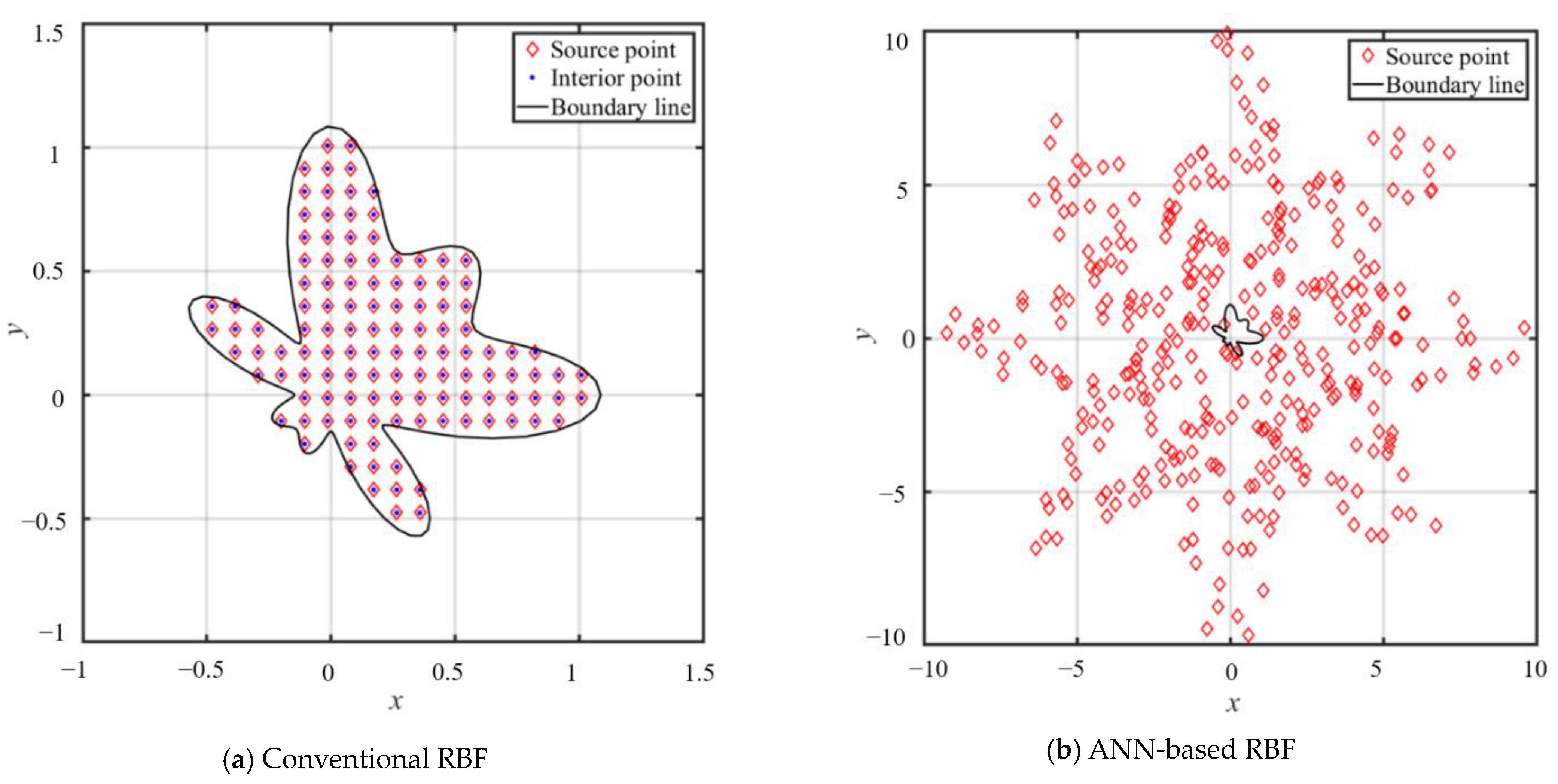
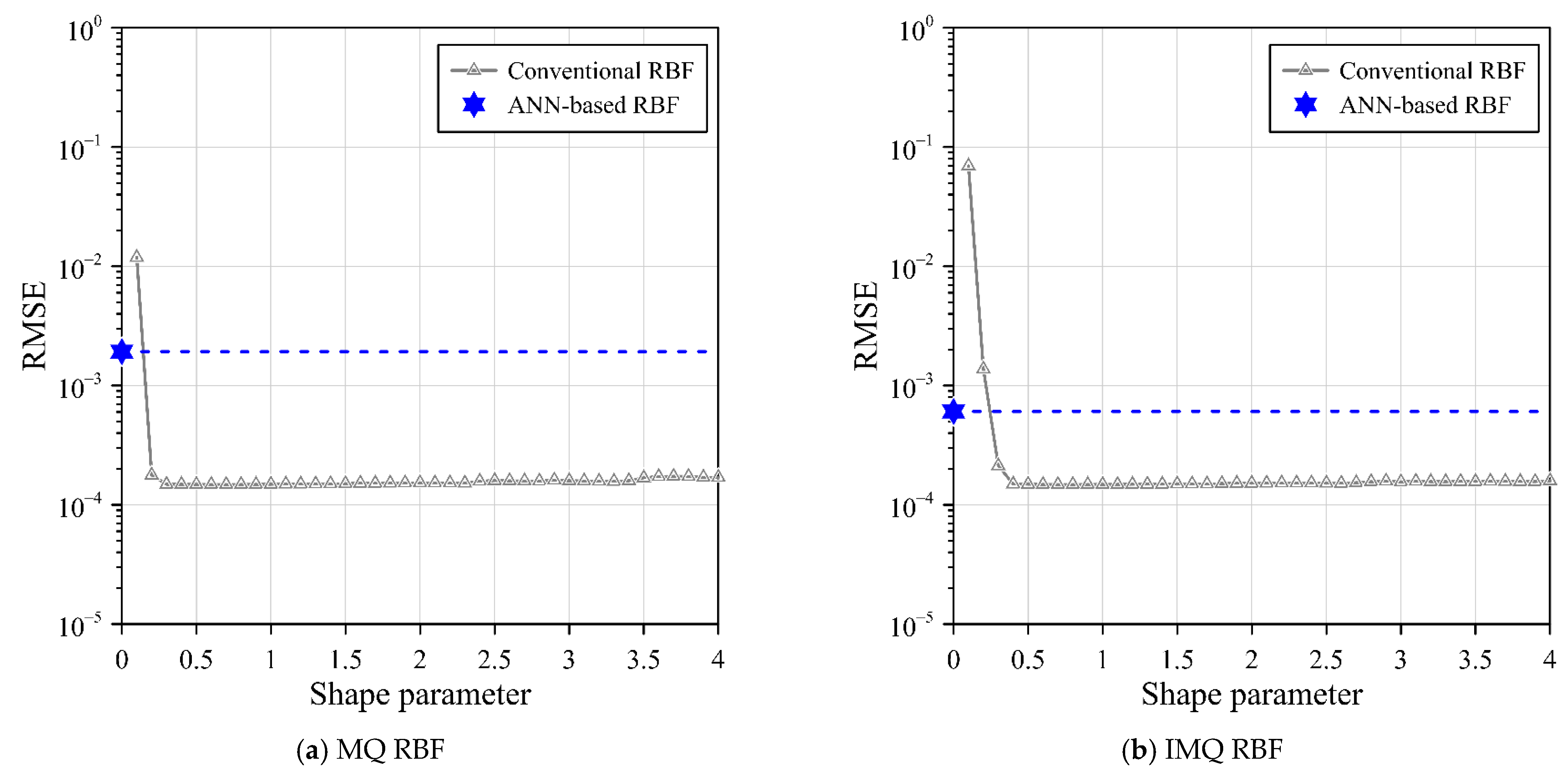
4.3. Example 3: Three-Dimensional Laplace Problem

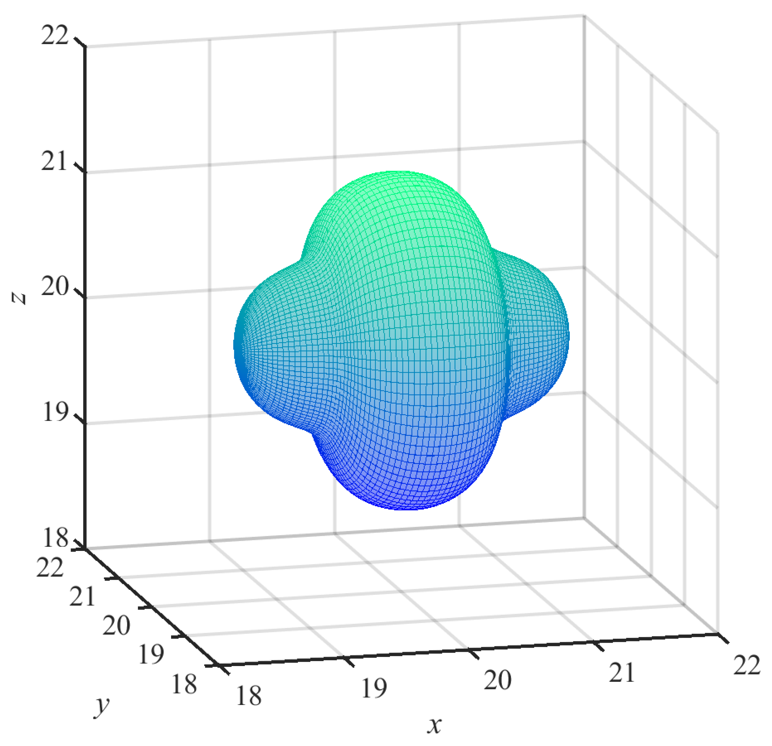
The domain for the three-dimensional Laplace problem is characterized by a complex and irregular boundary, as depicted in Figure 11. Within this intricate domain, the three-dimensional elliptic BVPs is mathematically described by Equation (1), where $A_x=A_y=A_z=B=f(x,y,z)=0$. The spherical parametric equation is denoted as follows:

$$\begin{array}{l}\partial \mathsf{\Omega }=\left\{(x,y,z)|x=\rho \left(\theta \right)\cos \theta , y=\rho \left(\theta \right)\sin \varphi \sin \theta , z=\rho \left(\theta \right)\cos \varphi \sin \theta \right\}, \\ \rho \left(\theta \right)={\left[\cos (4\theta )+\sqrt{4+{\sin }^2(4\theta )}\right]}^{1/4}.\end{array}$$

(24)

For this three-dimensional problem, the Dirichlet boundary conditions are enforced by applying the following analytical solution [14]

$$u(x,y,z)=\frac{1}{\sqrt{x^2+y^2+z^2}}.$$

(25)

Two different RBFs coupled with the MQ, IMQ, and Gaussian collocation methods are employed to address the problem at hand. In the conventional RBF collocation method, source points are uniformly distributed within the domain. The arrangement of the interior, source, and boundary points is such that the positions of the interior points perfectly align with those of the source points. In this configuration, a total of 900 source points, 576 interior points, and 325 boundary points are strategically positioned.

Alternatively, the ANN-based RBF collocation method adopts a different approach. We only need to position the boundary and source points. The source points are treated as fictitious centers dispersed randomly throughout the exterior domain. The use of exterior fictitious sources is governed by parametric equations, allowing for greater flexibility and versatility in addressing a wide range of practical problems.

The three-dimensional fictitious boundary is denoted as follows:

$$\partial {\mathsf{\Omega }}^s=\left\{(x_j^s,y_j^s,z_j^s)|x_j^s={\rho }_j^s\left({\theta }_j^s\right)\cos {\theta }_j^s\cos {\varphi }_j^s, y_j^s={\rho }_j^s\left({\theta }_j^s\right)\cos {\theta }_j^s\sin {\varphi }_j^s, z_j^s={\rho }_j^s\left({\theta }_j^s\right)s\mathrm{in}{\theta }_j^s\right\},$$

(26)

where ${\rho }_j^s({\theta }_j^s)=\eta \times \left\{[\frac{1}{8}\sin (9{\theta }_j^s)\sin (10{\varphi }_j^s)+0.5]\right\}, 0\le {\theta }_j^s\le 2\pi$, and ${\varphi }_j^s$ denotes the azimuth angle of the source points. $\eta$ is 5. A total of 900 source points and a total of 325 boundary points are used in the ANN-based RBF.

In the ANN-based RBF approach, the dataset was partitioned into distinct training, testing, and validation subsets, distributed in a ratio of 70% for training, 15% for testing, and 15% for validation. The proposed ANN-based RBF architecture comprised three hidden layers. The training process leveraged the Levenberg–Marquardt function, and the model’s performance evaluation was carried out using the mean-squared error. The outcomes reveal that by the 118th epoch, the validation performance, as assessed through the mean-squared error, reached an impressively low value of 10⁻¹⁸. Furthermore, the correlation coefficients for the training, validation, and testing datasets consistently yielded a value of 1. This exceptional correlation coefficient underscores the robust alignment between the exact solution and the predictions rendered by the proposed model. The results firmly establish the capacity of the proposed ANN-based RBF to effectively address the three-dimensional Laplace equation, emphasizing its proficiency and accuracy.

To facilitate comparative analysis, the RMSE and MAE metrics are employed to rigorously assess the precision of the computed outcomes. Subsequently, an in-depth evaluation of accuracy across three distinct RBFs ensues. The outcomes of this comparison are succinctly summarized in

Table 5. Results for the three-dimensional Laplace equation.

	RMSE		MAE
	Conventional RBF	ANN-Based RBF	Conventional RBF	ANN-Based RBF
MQ	1.91 × 10–9 (c = 1)	8.46 × 10–7 (without c)	2.17 × 10–8 (c = 1)	1.40 × 10–7 (without c)
IMQ	2.32 × 10–8 (c = 1.30)	6.11 × 10–6 (without c)	5.32 × 10–7 (c = 1.30)	8.45 × 10–7 (without c)
Gaussian	4.00 × 10–9 (c = 6.70)	5.24 × 10–5 (without c)	1.46 × 10–8 (c = 6.70)	2.33 × 10–4 (without c)

, presenting the RMSE and MAE values derived from conventional RBF and the proposed ANN-based RBF collocation method. Table 5 reveals that all variations of the ANN-based RBF collocation method, incorporating MQ, IMQ, and Gaussian RBFs while adopting exterior source points, yield commendably accurate outcomes. Specifically, the ANN-based RBF collocation method, when bolstered by exterior source points, yield highly accurate results, characterized by RMSE values of 10⁻⁷, 10⁻⁶, and 10⁻⁵, respectively.

The outcomes also serve to illustrate that the aforementioned simplified RBFs, augmented by exterior fictitious sources, are adeptly suited for resolving the intricacies of this three-dimensional Laplace problem with exceptional precision, as shown in Figure 12. Notably, the proposed ANN-based RBF collocation method’s characteristic lies in its ability to sidestep the discretization of the governing equation. This distinctive attribute underscores the inherent simplicity of the proposed ANN-based RBF collocation methodology, which effectively addresses elliptic BVPs through the utilization of provided boundary data and RBFs.

5. Conclusions

A novel approach for solving elliptic boundary value problems using an artificial-neural-network-based radial basis function collocation method is presented. The backpropagation neural network is employed, enabling learning from training data and enhancing accuracy. The principles of the proposed approach are thoroughly discussed, highlighting its conceptual foundations. Notable discoveries resulting from this study are summarized as follows.

• Discovering an appropriate shape parameter in RBFs for solving BVPs has consistently posed significant challenges, often requiring arduous efforts. In this investigation, we introduce an innovative approach—an ANN-based RBF collocation method that eliminates the need to explicitly determine the shape parameter. The proposed ANN-based RBFs offer distinct benefits, including uncomplicated mathematical formulations, enhanced accuracy, and straightforward implementation.
• Within the framework of the proposed ANN-based RBF collocation method, the training dataset comprises provided boundary data derived from accurate solutions and the radial distances spanning from exterior fictitious sources to boundary points. These distances play a pivotal role in constructing RBFs, such as multiquadric and inverse multiquadric RBFs. A distinctive advantage of the proposed ANN-based RBFs is its deliberate avoidance of discretizing the governing equation. This unique approach results in the proposed ANN-based RBF collocation method offering an uncomplicated path to addressing elliptic BVPs, requiring solely the input of boundary data and the chosen RBFs.
• The validation outcomes the proposed ANN-based RBF collocation method exemplify the remarkable performance of our approach across three simplified RBFs. Particularly noteworthy is its proficiency in solving Laplace-type equations across both two and three dimensions. Results demonstrate the effectiveness and efficiency of our proposed method, illustrating its capacity to yield precise solutions with minimal data input for addressing elliptic BVPs. Notably, the method hinges exclusively on given boundary data and the chosen RBFs. Further investigations are recommended to delve into the method’s characteristics when employed to solve various types of partial differential equations. Such studies would enable a comprehensive understanding of the approach’s adaptability and versatility across different problem domains.