Optimal Control of a Two-Patch Dengue Epidemic under Limited Resources

Abstract

Despite the ongoing preventive measures of vector control, dengue fever still presents outbreaks, and daily commuting of people also facilitates its propagation. To contain the disease spread after an outbreak has already occurred, the local healthcare authorities are compelled to perform insecticide spraying as a corrective measure of vector control, thus trying to avoid massive human infections. Several issues concerned with the practical implementation of such corrective measures can be solved from a mathematical standpoint, and the purpose of this study is to contribute to this strand of research. Using as a basis a two-patch dengue transmission ODE model, we designed the patch-dependent optimal strategies for the insecticide spraying with the optimal control approach. We also analyzed the response of the optimal strategies to three alternative modes of budget cuts under different intensities of daily commuting. Our approach illustrated that trying “to save money” by reducing the budget for corrective control is completely unwise, and the anticipated “savings” will actually turn into considerable additional public spending for treating human infections, which could have been averted by a timely corrective intervention.

1. Introduction

Dengue is a viral infection caused by the dengue virus (DENV1-DENV4), which is primarily transmitted to human individuals through the bite of infected Aedes aegypti and Aedes albopictus mosquitoes. Since only females need to ingest human blood to mature their eggs and male mosquitoes do not bite people, only the Aedes females are considered vectors of dengue and other mosquito-borne infections.

Tropical countries featuring the presence and abundance of Aedes mosquitoes usually carry the burden of dengue and other mosquito-borne viral infections in the human population. The local healthcare authorities conduct preventive control actions, such as eliminating mosquito breeding sites, stagnant water and rainwater treatment, environmental management, and educational campaigns targeting local communities, regardless of the presence or absence of disease outbreaks. However, these preventive measures cannot eliminate virus circulation, and disease outbreaks still occur.

To reduce the spread of dengue fever after an outbreak has already occurred, the local healthcare authorities need to implement the so-called corrective measure of vector control in order to curb the epidemics and contain the disease’s spread. Among the corrective actions, the most common is spreading insecticides in urban areas, excluding the interior of the houses. Notably, the costs of such actions are not usually anticipated in the yearly budget of local healthcare entities, and these actions are typically dependent on the available stock of the insecticide and human power needed to implement the spraying.

Among numerous questions regarding the practical implementation of corrective insecticide-based vector control measures, several issues can be solved from a mathematical standpoint, and the purpose of this study is to contribute to this strand of research. To make our study more realistic, we introduce a corrective control action modeling of the insecticide spraying into a two-patch model of dengue transmission that mimics the 2013 dengue outbreak in the city of Cali, Colombia, and its suburban areas [1]. This model has been thoroughly analyzed in the mentioned work, and its parameters have been estimated using the data gathered by the Municipal Secretariat of Public Health of Cali, Colombia.

The two-patch model in [1] was a good starting point because it considers daily commuting from suburban areas to Cali, using the Lagrange approach and residence times [2]. It is worth noting that the impact of daily commuting on the disease transmission was captured in other works (see, e.g., [3,4,5,6,7]); however, the design of patch-dependent strategies for corrective interventions based on insecticide spraying has not yet been addressed from the standpoint of dynamic optimization. In the present study, we derive the patch-dependent strategies for insecticide spraying using the optimal control framework, interpret their practical implementation, and estimate their underlying costs. We also show the resilience and robustness of the proposed strategies with respect to the intensity of people commuting. This result bears a remarkable value for the practical implementation of corrective control measures. Namely, healthcare entities may design the patch-dependent strategies for insecticide spraying basing only on the current state of the disease in both patches, and without estimating the actual number of daily commuters.

Following the approach developed in [8] for a one-patch model, we adjust the patch-dependent strategies for insecticide spraying to the budget restrictions imposed by healthcare entities. Generally speaking, the budget reductions can be made either in both patches or in only one of them. Here, it is pertinent to point out that the healthcare authorities usually prioritize corrective vector control in the big cities, thus neglecting the suburban areas. However, as our results show, those common practices are less cost-effective than their alternatives. In fact, they lead to a significant increase in the total public expenditures, i.e., the expenses for insecticide spraying and disease-related costs in the human population.

Lastly, we would like to emphasize that the present study is mainly focused on applying the optimal control methodology in the practical context of corrective vector control rather than exhibiting any new findings in the optimal control theory. From this standpoint, our results are expected to contribute to the practical aspects of the corrective disease control, whether featuring resource limitations or not, and the latter constitutes the primary novelty of our study. If the dengue outbreak has already begun, insecticide-based mosquito control is the most accessible and cost-effective measure to reduce the number of human infections and prevent further spread of the disease. In this context, our approach clearly illustrates that trying “to save money” at the beginning of dengue epidemics by reducing the budget for corrective control is entirely unwise and that such anticipated “savings” will turn into considerable additional public spending for treating human infections that could have been averted by a timely insecticide spraying at a much lower cost.

The paper is organized as follows. Section 2 provides the comprehensive description of the two-patch dengue transmission model originally introduced in [1]. In Section 3, we introduce two exogenous variables mimicking the insecticide spraying in both patches, formulate the optimal control problem of dynamic optimization, and justify the existence of its solution.

The main results are presented in Section 4, which consists of four subsections. Section 4.1 provides realistic data referring to the optimal control model that further allows us to estimate the total public expenditures related to the costs of corrective control strategies and the disease-related outlays. Section 4.2 provides numerical solutions of the optimal control problem with different commuting intensities when no budget limits are imposed. From these solutions, we estimate the costs necessary for implementing the optimal insecticide spraying in both patches. The situation when only a share of resources needed for implementing the corrective control strategies is available is thoroughly analyzed in Section 4.3, where we review three alternative modes of budget cuts combined with different intensities of daily commuting. The impact of the budget cut distributions between two patches on the disease propagation is examined in Section 4.4, and the modes of budget cuts corresponding to public expenditures combined with different intensities of daily commuting are estimated. From the latter, we conclude that the uniform budget reduction for both patches is the best way to act in resource-limited settings. Finally, Section 5 summarizes the key outcomes of the present work.

2. Two-Patch Dengue Transmission Model

Let us begin by revisiting the formulation of the two-patch dengue transmission model of the SEIR(S)-SEI type originally presented in [1]. This model was derived based on the following standard assumptions:

• The populations of human residents in both patches, $N_{h1}$ and $N_{h2}$, as well as the populations of vectors inhabiting both patches, $N_{v1}$ and $N_{v2}$, remain essentially invariant in time.
• All populations $N_{hi},N_{vi},i=1,2$ are homogeneous regarding susceptibility, exposure, and attraction.
• There is no dengue-induced mortality, neither for human individuals nor for vectors.
• Once DENV-infected, the mosquitoes never recover and stay infectious during their lifetime.
• There is no vertical DENV transmission, so all the newborns (humans and vectors) are DENV-free.
• Human individuals can move between the patches, while mosquitoes remain in the same patch during their lifetime.

The total populations of human individuals $N_{hi},i=1,2$ residing in each patch are subdivided into four disjoint classes: susceptible (DENV-free people), exposed (DENV-carrying people who are not infectious yet), infectious (DENV-carrying people who are capable of transmitting the virus to female mosquitoes during the bite), and individuals recovered from the disease. The fractions of the corresponding human groups regarding the total populations $N_{hi},i=1,2$ residing in each patch are denoted with $S_{hi}, E_{hi}, I_{hi},$ and $R_{hi},$ respectively. In turn, the total populations of vectors $N_{vi},i=1,2$ inhabiting each patch are subdivided into three disjoint classes: susceptible (DENV-free female mosquitoes), exposed (DENV-carrying female mosquitoes which are not infectious yet), and infectious (DENV-carrying female mosquitoes which are capable of transmitting the virus to human individuals during the bite). The fractions of the corresponding groups of vectors regarding the total populations $N_{vi},i=1,2$ inhabiting each patch are denoted with $S_{vi}, E_{vi},$ and $I_{vi},$ respectively. Notably, all the population fractions or proportions introduced above vary in time and satisfy the following relationships valid for all $t\ge 0$:

$$S_{hi}+E_{hi}+I_{hi}+R_{hi}=1,S_{vi}+E_{vi}+I_{vi}=1,i=1,2.$$

(1)

Numerous studies have confirmed that dengue disease caused by any of the four dengue serotypes DENV1-DENV4 might result either in asymptomatic infection or range from mild febrile illness with flu-like symptoms to severe dengue or dengue shock syndrome (DSS). There are no exact estimations of the proportion of asymptomatic infections among all dengue morbidity, but they may be even higher in density than the symptomatic cases [9,10,11]. Therefore, we may assume that some infectious human individuals from the classes $I_{hi},i=1,2$ may exhibit no symptoms and be unaware of being contagious. Such people may commute between the two patches and contribute to the disease spreading.

To model the demographic changes while keeping the populations of humans and vectors essentially invariant over time, we assume that both human populations $N_{hi},i=1,2$ and both vector populations $N_{vi},i=1,2$ have equal birth and death rates. Namely, the human birth and death rate is denoted by ${\mu }_h$, while the birth and death rate for mosquitoes is denoted by ${\mu }_v$. For convenience,

Table 1. Description of the model’s parameters with values borrowed from [1] (epidemic scenario).

Parameter	Description	Units	Assumed Value
${\kappa }_v$	Latent-to-infectious conversion rate in vectors	day${}^{-1}$	$1/8$
${\kappa }_h$	Latent-to-infectious conversion rate in humans	day${}^{-1}$	$1/4$
$\gamma$	Rate of human recovery	day${}^{-1}$	$1/6$
${\mu }_v$	Per capita vector birth/death rate	day${}^{-1}$	$1/30$
${\mu }_h$	Per capita of human births/deaths	day${}^{-1}$	$1/(75\times 365)$
$\alpha$	Mosquito biting rate	day${}^{-1}$	$0.4517$
$\tau$	Reinfection rate for human individuals	day${}^{-1}$	$0.0262$
$p_v$	Human-to-vector transmission probability of the pathogen	–	$0.2378$
$p_h$	Vector-to-human transmission probability of the pathogen	–	$0.219$

summarizes the descriptions of all baseline parameters related to disease transmission dynamics.

The exposed or latent human and vector individuals from the classes $E_{hi}$ and $E_{vi},i=1,2$ become infectious after the virus incubation period and then pass to the classes $I_{hi}$ and $I_{vi},i=1,2,$ respectively. We suppose the intrinsic and extrinsic virus incubation (in humans and mosquitoes) lasts for $1/{\kappa }_h$ and $1/{\kappa }_v$ days, respectively. Thus, the conversion rates from latency to infectiousness are denoted by ${\kappa }_h$ and ${\kappa }_v$ for humans and vectors, respectively.

We also assume that the recovery from the disease takes $1/\gamma$ days, and the recovered individuals become susceptible to heterologous DENV serotypes after $1/\tau$ days if various DENV serotypes circulate simultaneously in the environment. Notably, no reinfection is expected under the strong dominance of only one homologous DENV serotype, and in such a case, it is supposed that $\tau =0$.

It is worthwhile to point out that the susceptible vectors inhabiting Patch 1 (resp. Patch 2) may acquire the virus after biting either an infectious human resident from class $I_{h1}$ (resp. class $I_{h2}$) or an asymptomatic visitor to Patch 1 (resp. Patch 2) belonging to the class $I_{h2}$ (resp. class $I_{h1}$). Similarly, the susceptible human individuals residing in Patch 1 (resp. Patch 2) may acquire the virus after being bitten by either an infectious vector from their home patch, belonging to the class $I_{v1}$ (resp. $I_{v2}$), or by an infectious vector from the other patch $I_{v2}$ (resp. $I_{v1}$) while visiting Patch 2 (resp. Patch 1). Thus, it becomes clear that people commuting between the two patches may affect the virus transmission, even though all vectors remain in their home patches.

The commuting of people between two patches is modeled using the so-called Lagrangian approach [2,3], under which the movement of individuals between patches is mimicked in terms of their residence times, i.e., the shares of time spent at each patch. Let

$$Q=\left(\begin{array}{cc}{q}_{11}& q_{12}\\ q_{21}& q_{22}\end{array}\right)$$

(2)

denote the residence time matrix [3] that couples both patches and whose elements $q_{ij}$ express the shares or fractions of time a person residing in Patch i spends, on average, in Patch j. Notably, the elements of Q satisfy the following relationships:

$$0\le q_{ij}\le 1,\sum _{j=1}^2{q}_{ij}=1,i,j=1,2.$$

Using the elements of (2) and following the idea exposed in [2], we introduce another matrix

$$P=\left(\begin{array}{cc}{P}_{11}& P_{12}\\ P_{21}& P_{22}\end{array}\right)=\left(\begin{array}{cc}{\displaystyle \frac{q_{11}{N}_{h1}}{q_{11}{N}_{h1}+q_{21}{N}_{h2}}}& {\displaystyle \frac{q_{12}{N}_{h1}}{q_{12}{N}_{h1}+q_{22}{N}_{h2}}}\\ {\displaystyle \frac{q_{21}{N}_{h2}}{q_{11}{N}_{h1}+q_{21}{N}_{h2}}}& {\displaystyle \frac{q_{22}{N}_{h2}}{q_{12}{N}_{h1}+q_{22}{N}_{h2}}}\end{array}\right),$$

(3)

which is referred to as the matrix of effective residence times, since its components are defined in terms of the elements of the residence times matrix Q (see (2)), weighted by the respective shares or proportions of the effective population sizes at each patch. Notably, the elements of P satisfy the following relationships:

$$0\le P_{ij}\le 1,\sum _{i=1}^2{P}_{ij}=1,i,j=1,2$$

and they express the proportions of the residents from Patch i effectively present in Patch j. For example, $P_{12}$ is the fraction of residents of Patch 1 who visit Patch 2 (that is, $q_{12}{N}_{h1}$) relative to the effective population size of Patch 2 (which is equal to $q_{12}{N}_{h1}+q_{22}{N}_{h2}$).

To model the disease incidence, we recall from other works (see, e.g., [1,2,3]) that the per capita “human-to-vector” virus transmission rate ${\beta }_v$ is usually assumed to be proportional to the mosquito biting rate $\alpha$ and the probability $p_v\in [0,1]$ of the virus transmission, that is, ${\beta }_v=\alpha p_v$. Here, the mosquito biting rate refers to the number of times a female mosquito needs to have a blood meal by biting people on average daily. As the parameters $\alpha$ and $p_v$ are unaffected by the people’s movements, the same “human-to-vector” virus transmission rate ${\beta }_v$ can be assumed for both patches.

Usually, for a female mosquito, it suffices to bite one person for having her blood meal. On the other hand, the same person may receive bites from more than one female mosquito. Therefore, the “vector-to-human” virus transmission rate ${\beta }_h$ depends not only on the mosquito biting rate $\alpha$ and the probability $p_h\in [0,1]$ of the virus transmission but also on the so-called vectorial density, i.e., the average number of female mosquitoes per one human individual. Even though all vectors stay in their patches and both vector populations $N_{vi}$ remain essentially invariant, the number of human individuals effectively present at each patch varies when people are commuting between the patches. Therefore, the “vector-to-human” virus transmission rate ${\beta }_h$ depends on the so-called effective vectorial density at each patch [1]. The latter can be defined using the components of the residence time matrix Q in the following way:

$$\mathrm{Patch}1\text{:}{\displaystyle \frac{N_{v1}}{q_{11}{N}_{h1}+q_{21}{N}_{h2}}},\mathrm{Patch}2\text{:}{\displaystyle \frac{N_{v2}}{q_{12}{N}_{h1}+q_{22}{N}_{h2}}}$$

(4)

Thus, the effective vectorial density expresses an average number of female mosquitoes in Patch j per one human individual effectively present in Patch j for $j=1,2.$ Using the quantities defined by (4), the patch-dependent “vector-to-human” contact rates ${\beta }_{hi},i=1,2$ can be written as follows:

$${\beta }_{h1}={\displaystyle \frac{\alpha p_h{N}_{v1}}{q_{11}{N}_{h1}+q_{21}{N}_{h2}}},{\beta }_{h2}={\displaystyle \frac{\alpha p_h{N}_{v2}}{q_{12}{N}_{h1}+q_{22}{N}_{h2}}}.$$

(5)

Finally, the normalized two-patch dengue transmission model can be written as a dynamical system of fourteen ordinary differential equations:

$$\begin{array}{cc}\hfill {\dot{S}}_{v1}\left(t\right)& ={\mu }_v-{\beta }_v{S}_{v1}\left(t\right)\left[\sum _{j=1}^2{P}_{j1}{I}_{hj}\left(t\right)\right]-{\mu }_v{S}_{v1}\left(t\right)\hfill \\ \hfill {\dot{E}}_{v1}\left(t\right)& ={\beta }_v{S}_{v1}\left(t\right)\left[\sum _{j=1}^2{P}_{j1}{I}_{hj}\left(t\right)\right]-({\mu }_v+{\kappa }_v)E_{v1}\left(t\right)\hfill \\ \hfill {\dot{I}}_{v1}\left(t\right)& ={\kappa }_v{E}_{v1}\left(t\right)-{\mu }_v{I}_{v1}\left(t\right)\hfill \\ \hfill {\dot{S}}_{h1}\left(t\right)& ={\mu }_h-S_{h1}\left(t\right)\left[\sum _{j=1}^2{\beta }_{hj}{q}_{1j}{I}_{vj}\left(t\right)\right]-{\mu }_h{S}_{h1}\left(t\right)+\tau R_{h1}\left(t\right)\hfill \\ \hfill {\dot{E}}_{h1}\left(t\right)& =S_{h1}\left(t\right)\left[\sum _{j=1}^2{\beta }_{hj}{q}_{1j}{I}_{vj}\left(t\right)\right]-({\mu }_h+{\kappa }_h)E_{h1}\left(t\right)\hfill \\ \hfill {\dot{I}}_{h1}\left(t\right)& ={\kappa }_h{E}_{h1}\left(t\right)-(\gamma +{\mu }_h)I_{h1}\left(t\right)\hfill \\ \hfill {\dot{R}}_{h1}\left(t\right)& =\gamma I_{h1}\left(t\right)-({\mu }_h+\tau )R_{h1}\left(t\right)\hfill \\ \hfill {\dot{S}}_{v2}\left(t\right)& ={\mu }_v-{\beta }_v{S}_{v2}\left(t\right)\left[\sum _{j=1}^2{P}_{j2}{I}_{hj}\left(t\right)\right]-{\mu }_v{S}_{v2}\left(t\right)\hfill \\ \hfill {\dot{E}}_{v2}\left(t\right)& ={\beta }_v{S}_{v2}\left(t\right)\left[\sum _{j=1}^2{P}_{j2}{I}_{hj}\left(t\right)\right]-({\mu }_v+{\kappa }_v)E_{v2}\left(t\right)\hfill \\ \hfill {\dot{I}}_{v2}\left(t\right)& ={\kappa }_v{E}_{v2}\left(t\right)-{\mu }_v{I}_{v2}\left(t\right)\hfill \\ \hfill {\dot{S}}_{h2}\left(t\right)& ={\mu }_h-S_{h2}\left(t\right)\left[\sum _{j=1}^2{\beta }_{hj}{q}_{2j}{I}_{vj}\left(t\right)\right]-{\mu }_h{S}_{h2}\left(t\right)+\tau R_{h2}\left(t\right)\hfill \\ \hfill {\dot{E}}_{h2}\left(t\right)& =S_{h2}\left(t\right)\left[\sum _{j=1}^2{\beta }_{hj}{q}_{2j}{I}_{vj}\left(t\right)\right]-({\mu }_h+{\kappa }_h)E_{h2}\left(t\right)\hfill \\ \hfill {\dot{I}}_{h2}\left(t\right)& ={\kappa }_h{E}_{h2}\left(t\right)-(\gamma +{\mu }_h)I_{h2}\left(t\right)\hfill \\ \hfill {\dot{R}}_{h2}\left(t\right)& =\gamma I_{h2}\left(t\right)-({\mu }_h+\tau )R_{h2}\left(t\right)\hfill \end{array}$$

where dots in the left-hand sides denote the derivative with respect to time, that is,

$$\dot{X}\left(t\right):={\displaystyle \frac{dX}{dt}}.$$

The above-formulated two-patch dengue transmission model was thoroughly studied in [1] under different human mobility scenarios and without vector control measures. In the sequel, this model will serve as a basis for testing different strategies of vector control intervention applied in both patches. The following section encompasses the formulation of dengue control problem from the standpoint of optimal control.

3. Optimal Control Approach

As millions of people worldwide are exposed to the risk of vector-borne infections, dengue control is a collective effort involving individuals, communities, healthcare systems, and government authorities. With several types of vaccines against all DENV serotypes still under development [12], the disease control efforts continue targeting the reduction in the local mosquito density. Vector control actions conducted by local healthcare authorities in dengue-endemic areas can be divided into two majors groups:

• Preventive actions include eliminating mosquito breeding sites, stagnant water and rainwater treatment, environmental management, and educational campaigns targeting local communities. These are routine interventions carried out regardless of the presence or absence of disease outbreaks.
• Corrective actions, such as insecticide spraying, are conducted as part of an emergency response to curb the disease outbreak or a cluster of identified cases in a particular area.

In the present study, we will address the second group of control actions from the standpoint of dynamic optimization and accounting for people commuting between two patches. Taking as an example the epidemiological situation of dengue in the city of Cali and its suburbs (Republic of Colombia), we will try to model the current practices of local healthcare authorities for implementing corrective control actions seeking eventual suppression of dengue cases in the city. As the corrective measures do not always have a sufficient budget, we will also address the flexibility and robustness of corrective actions under budget constraints.

To model the corrective control actions of insecticide spraying applied in both patches, we introduce two exogenous variables $u_i\left(t\right)\in [0,1], i=1,2, t\in [0,T]$ where $T>0$ denotes the time horizon. These variables $u_1\left(t\right)$ and $u_2\left(t\right)$ will directly affect the mosquito mortality rate, ${\mu }_v$, in both patches. However, as the model presented in Section 2 is normalized, the variables $u_i\left(t\right), i=1,2$ should also be scaled accordingly while bearing a meaningful relation to the amount of insecticide sprayed.

To derive a meaningful definition of $u_i\left(t\right), i=1,2$, it is worthwhile to recall that there are generally accepted norms and guidelines for daily insecticide spraying regarding the volume of insecticide used. Specific regulations may vary based on the type of insecticide, target mosquito species, and local environmental policies. One of the key indicators is the so-called insecticide application rate. It refers to the amount of a diluted insecticide (volume) applied daily per unit area. Let $v_i\left(t\right)\in [0,D], i=1,2$ represent the total volume of a diluted insecticide destined for application in Patch i on day t, and let $D>0$ denote the maximal volume of insecticide that is allowed for daily application over a unit area at each patch. Thus, the exogenous variables $u_i\left(t\right), i=1,2$ can be viewed as

$$u_i\left(t\right)={\displaystyle \frac{v_i\left(t\right)}{\left(\mathrm{area}\mathrm{of}\mathrm{Patch}i\right)\times D}},i=1,2.$$

(6)

Under the above definition, $u_1\left(t\right)$ and $u_2\left(t\right)$ become dimensionless and acquire meaningful interpretations. For instance, $u_1\left(t\right)=1, u_2\left(t\right)=0.5$ implies that, on day t, the maximal allowed volume of a diluted insecticide should be uniformly sprayed in Patch 1, while only $50\%$ of the maximal allowed volume should be uniformly spread in Patch 2.

It is worthwhile to point out that the maximum volume of insecticide allowed for daily application over a unit area (denoted by D) may vary depending on the insecticide dilution. The concentration of the insecticide also defines the insecticide’s level of toxicity or lethality for target mosquito species and usually ranges between $20\%$ and $90\%$ [13]. In the sequel, the insecticide lethality will be denoted by $\eta \in (0,1)$, while it is also understood that smaller values of $\eta$ will require a larger volume $v_i\left(t\right), i=1,2$ of diluted insecticide and the constant D may take larger values (cf. (6)). In accordance with definition (6), we can determine the so-called set of admissible controls as $\mathcal{U}:=[0,1]\times [0,1]$.

As insecticide spraying is a corrective measure of vector control, healthcare authorities may consider applying this type of intervention when there is a significant increase in dengue cases among the human population. Thus, the ultimate purpose of insecticide spraying consists in containing dengue epidemics. Still, the effect of this control action is not immediate and can be observed within 15–30 days after the insecticide spraying begins. It is worth pointing out that the duration and frequency of insecticide-spraying campaigns depend on the environmental norms (expressed by the quantity D) and other factors, such as the total stock of insecticides, available personnel, equipment, etc. Hence, this type of intervention is usually limited in terms of costs and time and may continue only for several days at most.

Therefore, the global challenge for the healthcare authorities consists in choosing an optimal strategy for insecticide spraying in both patches, $\left(u_1^{*}\left(t\right),u_2^{*}\left(t\right)\right)\in \mathcal{U}, t\in [0,T]$, that minimizes the total costs associated with human infections during the dengue outbreak together with the overall costs of control interventions while meeting the budget constraint whenever such a constraint is imposed. From the mathematical standpoint, this goal can be expressed by the following objective functional:

$$J\left(u_1\left(t\right),u_2\left(t\right)\right)=\underset{0}{\overset{T}{\int }}\left[W_1{N}_{h1}{I}_{h1}\left(t\right)+W_2{N}_{h2}{I}_{h2}\left(t\right)+W_3{A}_1{u}_1\left(t\right)+W_4{A}_2{u}_2\left(t\right)\right]dt,$$

(7)

where $N_{hi},i=1,2$ refer to the total human populations residing in both patches and $A_i,i=1,2$ denote their areas. Here, the weight coefficients $W_1,W_2$ express the medical and societal cost related to one human infection, while $W_3,W_4$ stand for the cost of insecticide spraying per unit of area.

Thus, the dynamic optimization problem can be formulated as minimizing the objective functional (7), that is,

$$\underset{(u_1,u_2)\in \mathcal{U}}{min}J\left(u_1\left(t\right),u_2\left(t\right)\right)$$

(8)

subject to

$$\begin{array}{cc}\hfill {\dot{S}}_{vi}\left(t\right)& ={\mu }_v-{\beta }_v{S}_{vi}\left(t\right)\left[\sum _{j=1}^2{P}_{ji}{I}_{hj}\left(t\right)\right]-\left({\mu }_v+\eta u_i\left(t\right)\right)S_{vi}\left(t\right)\hfill \end{array}$$

(9a)

$$\begin{array}{cc}\hfill {\dot{E}}_{vi}\left(t\right)& ={\beta }_v{S}_{vi}\left(t\right)\left[\sum _{j=1}^2{P}_{ji}{I}_{hj}\left(t\right)\right]-\left({\mu }_v+{\kappa }_v+\eta u_i\left(t\right)\right)E_{vi}\left(t\right)\hfill \end{array}$$

(9b)

$$\begin{array}{cc}\hfill {\dot{I}}_{vi}\left(t\right)& ={\kappa }_v{E}_{vi}\left(t\right)-\left({\mu }_v+\eta u_i\left(t\right)\right)I_{vi}\left(t\right)\hfill \end{array}$$

(9c)

$$\begin{array}{cc}\hfill {\dot{S}}_{hi}\left(t\right)& ={\mu }_h-S_{hi}\left(t\right)\left[\sum _{j=1}^2{\beta }_{hj}{q}_{ij}{I}_{vj}\left(t\right)\right]-{\mu }_h{S}_{hi}\left(t\right)+\tau R_{hi}\left(t\right)\hfill \end{array}$$

(9d)

$$\begin{array}{cc}\hfill {\dot{E}}_{hi}\left(t\right)& =S_{hi}\left(t\right)\left[\sum _{j=1}^2{\beta }_{hj}{q}_{ij}{I}_{vj}\left(t\right)\right]-({\mu }_h+{\kappa }_h)E_{hi}\left(t\right)\hfill \end{array}$$

(9e)

$$\begin{array}{cc}\hfill {\dot{I}}_{hi}\left(t\right)& ={\kappa }_h{E}_{hi}\left(t\right)-(\gamma +{\mu }_h)I_{hi}\left(t\right)\hfill \end{array}$$

(9f)

$$\begin{array}{cc}\hfill {\dot{R}}_{hi}\left(t\right)& =\gamma I_{hi}\left(t\right)-({\mu }_h+\tau )R_{hi}\left(t\right)\hfill \end{array}$$

(9g)

$$\left(S_{vi}\left(0\right),E_{vi}\left(0\right),I_{vi}\left(0\right),S_{hi}\left(0\right),E_{hi}\left(0\right),I_{hi}\left(0\right),R_{hi}\left(0\right)\right)\ne (1,0,0,1,0,0,0),i=1,2$$

(9h)

and $(u_1,u_2)\in \mathcal{U}$ implies that

$$0\le u_i\left(t\right)\le 1,\forall t\in [0,T],i=1,2.$$

(10)

It is important to highlight that the initial conditions (9h) are nonnegative, have constant values between 0 and 1, and satisfy the following relationships:

$$S_{hi}\left(0\right)+E_{hi}\left(0\right)+I_{hi}\left(0\right)+R_{hi}\left(0\right)=1,S_{vi}\left(0\right)+E_{vi}\left(0\right)+I_{vi}\left(0\right)=1,i=1,2.$$

(11)

Numerical values given in (9h) correspond to the initial proportions of the vector and human populations in both patches before the control intervention begins. Furthermore, the control functions (10) are assumed to be piecewise continuous.

The necessary condition for the solvability of the optimal control problem (8)–(10) is the solvability of the dynamical system (9) with any admissible controls (10). The following statement gives the validity of this condition.

Proposition 1. 

For each pair of piecewise continuous real functions given by (10), the initial value problem (9) has a unique solution defined for all $t\ge 0$ and $T>0$, while all the components of this solution remain within the range $[0,1]$.

Proof. 

Let $\mathbf{X}=\left({\mathbf{X}}^1,{\mathbf{X}}^2\right)\in {\mathbb{R}}_{+}^{14}$ denote the vector of the state variables of the dynamical system (9), where ${\mathbf{X}}^i=\left(S_{vi},E_{vi},I_{vi},S_{hi},E_{hi},I_{hi},R_{hi}\right), i=1,2$. The controlled system (9) can then be written in the form

$$\dot{\mathbf{X}}\left(t\right)=\mathbf{F}\left(\mathbf{X}\left(t\right),u_1\left(t\right),u_2\left(t\right)\right),$$

where $\mathbf{F}\left(\mathbf{X}\left(t\right),u_1\left(t\right),u_2\left(t\right)\right)$ is the vector field corresponding to the right-hand sides of Equation (9). Let $\mathbf{X}(t;u_1,u_2)$ denote the solution to (9) corresponding to $(u_1,u_2)\in \mathcal{U}$.

In the absence of control intervention, that is, when $u_1=u_2=0$, it was shown in [1] that the dynamical system (9) has a unique nonnegative solution $\mathbf{X}(t;0,0)$ engendered by any initial conditions complying with (11). Furthermore, this solution continuously depends on the initial conditions, can be extended for all $t\ge 0$, and its components satisfy the relationships (1) while staying within the range $[0,1]$.

Moreover, as $\mathbf{F}\left(\mathbf{X}\left(t\right),u_1\left(t\right),u_2\left(t\right)\right)$ remains continuous and locally Lipschitz in $\mathbf{X}$ for each pair $(u_1,u_2)\in \mathcal{U}$, a unique solution to (9) exists for all $u_i\left(t\right),i=1,2$ defined by (10) for any $T>0$. More details regarding this standard result can be consulted in [14,15] or similar textbooks. Notably, the right-hand sides of the dynamical system (9) are non-increasing with respect to the exogenous variables $u_i,i=1,2$. Therefore, the growth rate $\mathbf{F}\left(\mathbf{X}\left(t\right),u_1\left(t\right),u_2\left(t\right)\right)$ with $u_i\in (0,1],i=1,2$ is smaller than $\mathbf{F}\left(\mathbf{X}\left(t\right),0,0\right)$. Thus, all the components of the solution to (9) with $(u_1,u_2)\in \mathcal{U}$ are also bounded and remain within the range $[0,1]$.  □

Once the solvability of the controlled dynamical system (9) is established for all admissible controls $(u_1,u_2)\in \mathcal{U}$, we proceed to formulate the following statement for ensuring the solvability of the optimal control problem (8)–(10).

Proposition 2. 

There exists a pair of optimal controls $\left(u_1^{*}\left(t\right),u_2^{*}\left(t\right)\right)$ satisfying (10), and the corresponding solutions $\left(S_{vi}^{*}\left(t\right),E_{vi}^{*}\left(t\right),I_{vi}^{*}\left(t\right),S_{hi}^{*}\left(t\right),E_{hi}^{*}\left(t\right),I_{hi}^{*}\left(t\right),R_{hi}^{*}\left(t\right)\right), i=1,2$ of the initial value problem (9), which minimize the functional (7).

Proof. 

To formally prove the existence of the optimal controls, we make use of the standard existence result given [16] and verify that all the hypotheses established are satisfied for the optimal control problem (8)–(10). In this context, we point out the validity of the following statements:

(i)

In view of Proposition 1, the state trajectories $\mathbf{X}(t;u_1,u_2)$ of the controlled dynamical system (9) are bounded for all admissible controls $\left(u_1,u_2\right)\in \mathcal{U}$ and for all $t\ge 0.$

(ii)

The set $\mathcal{U}=[0,1]\times [0,1]$ of admissible controls is compact and convex in ${\mathbb{R}}_{+}^2$.

(iii)

The right-hand sides of the dynamical system (9) are linear with respect to $u_1$ and $u_2$.

(iv)

The set of all possible initial states $\mathbf{X}\left(0\right)$ and the set of all possible terminal states $\mathbf{X}\left(T\right),0<T<\infty$ are both compact because each state variable remains within the range $[0,1]$ for all $t\ge 0.$

(v)

As the integrand of the objective functional (7) is linear with respect to $u_1$ and $u_2$, it is also convex in $u_1, u_2$ and is bounded from below.

Conditions (i)–(v) indicate that the sufficient conditions for the existence of optimal controls formulated in [16] (see Theorem 4.1 and Corollary 4.1, pp. 68–69) are satisfied. This ensures the existence of $u_1^{*}:[0,T]\mapsto [0,1]$ and $u_2^{*}:[0,T]\mapsto [0,1]$ that minimize functional (7) over any finite time interval $t\in [0,T],0<T<\infty$.  □

The optimal control problem (8)–(10) has fourteen state variables plus two control variables. Due to its high dimensionality, there are no prospects of obtaining an exact solution in the closed form; therefore, the optimal control problem (8)–(10) can only be solved numerically. Before we proceed to present its numerical solutions (Section 4), let us expose some arguments concerning the form of the optimal strategies $\left(u_1^{*}\left(t\right),u_2^{*}\left(t\right)\right)$ and their interpretations.

Knowing from Proposition 2 that the optimal solution exists and observing that the right-hand sides of the dynamical system (9), as well as the integrand of the objective functional (7), are linear with respect to $u_1,u_2$, one may expect an optimal solution in the bang-bang form. Notably, the bang-bang form of optimal controls fully agrees with the common practices of insecticide-spreading campaigns in many countries affected by dengue and other mosquito-borne diseases [8].

By formally applying the solution procedure based on the Pontryagin minimum principle (see, e.g., [17] or similar textbooks), we define the Hamiltonian corresponding to the optimal control problem (8)–(10) that has the following form:

$$H(\mathsf{\Lambda },\mathbf{X},u_1,u_2)=W_1{N}_{h1}{I}_{h1}+W_2{N}_{h2}{I}_{h2}+W_3{A}_1{u}_1+W_4{A}_2{u}_2+〈\mathsf{\Lambda }\left(t\right),\mathbf{F}\left(\mathbf{X},u_1,u_2\right)〉,$$

(12)

where $\langle ·,·\rangle$ stands for scalar product and $\mathsf{\Lambda }=\left({\mathsf{\Lambda }}^1,{\mathsf{\Lambda }}^2\right)\in {\mathbb{R}}^{14}, {\mathsf{\Lambda }}^i=({\lambda }_{1i},\dots ,{\lambda }_{7i}), i=1,2$ denotes the vector of adjoint or co-state variables corresponding to the state variables $\mathbf{X}=\left({\mathbf{X}}^1,{\mathbf{X}}^2\right), {\mathbf{X}}^i=\left(S_{vi},E_{vi},I_{vi},S_{hi},E_{hi},I_{hi},R_{hi}\right), i=1,2$. Here, the co-state vector function $\mathsf{\Lambda }\left(t\right)$ is absolutely continuous [17] and satisfies the adjoint ODE system with transversality condition

$$\dot{\mathsf{\Lambda }}\left(t\right)=-{\displaystyle \frac{\partial H}{\partial \mathbf{X}}},\mathsf{\Lambda }\left(T\right)=\mathbf{0}.$$

(13)

The detailed form of the adjoint system (13) is given in Appendix A.

In view of Proposition 2, the optimal control problem (8)–(10) has an optimal solution, say $\left(u_1^{*}\left(t\right),u_2^{*}\left(t\right)\right)\in \mathcal{U}$, which is defined for all $t\in [0,T], 0<T<\infty$. This solution, together with the corresponding optimal state ${\mathbf{X}}^{*}\left(t\right)=\mathbf{X}\left(t;u_1^{*}\left(t\right),u_2^{*}\left(t\right)\right)$ and the underlying co-state $\mathsf{\Lambda }\left(t\right)$ satisfying the adjoint ODE system (13), must comply with the necessary condition of optimality in the form of the Pontryagin minimum principle. In other words, the Hamiltonian (12) must satisfy the following condition almost at each $t\in [0,T]$ along the optimal path ${\mathbf{X}}^{*}\left(t\right)$:

$$H\left(\mathsf{\Lambda },{\mathbf{X}}^{*},u_1^{*},u_2^{*}\right)\le H\left(\mathsf{\Lambda },{\mathbf{X}}^{*},u_1,u_2\right),\forall (u_1,u_2)\in \mathcal{U}.$$

As the Hamiltonian is linear with respect to $u_1$ and $u_2$, we have that its partial derivatives

$${\displaystyle \frac{\partial H}{\partial u_i}}=W_{2+i}{A}_i-\eta \left[{\lambda }_{1i}{S}_{vi}+{\lambda }_{2i}{E}_{vi}+{\lambda }_{3i}{I}_{vi}\right],i=1,2$$

(14)

are independent of $u_1$ and $u_2$ and, generally speaking, the Hamiltonian attains its minimum with respect to $u_i, i=1,2$ at the extreme points of the interval $[0,1]$. Then we can derive that

$$u_i^{*}\left(t\right)=\left\{\begin{array}{ccc}0\hfill & \mathrm{if}& {\phi }_i\left(t\right)>0\\ 1\hfill & \mathrm{if}& {\phi }_i\left(t\right)<0\end{array}\right.i=1,2$$

(15)

where

$${\phi }_i\left(t\right):=W_{2+i}{A}_i-\eta \left[{\lambda }_{1i}\left(t\right)S_{vi}^{*}\left(t\right)+{\lambda }_{2i}\left(t\right)E_{vi}^{*}\left(t\right)+{\lambda }_{3i}\left(t\right)I_{vi}^{*}\left(t\right)\right],i=1,2,$$

(16)

denote the switching functions which represent the right-hand sides of the relationships in (14) evaluated at each $t\in [0,T].$ Thus, the optimal control $u_i^{*}\left(t\right), i=1,2$ is piecewise constant and switches between the “on” and “off” modes expressed by $u_i^{*}\left(t\right)=1$ and $u_i^{*}\left(t\right)=0$, respectively. The number of switches equals the number of roots of the switching function ${\phi }_i\left(t\right)$. However, if there exists an interval $[t_1,t_2]\subseteq [0,T], t_1<t_2$ within which it holds that ${\phi }_i\left(t\right)\equiv 0, t\in [t_1,t_2]$, there is a possibility that the optimal control is interior, that is, $0<u_i^{*}\left(t\right)<1, t\in [t_1,t_2]$.

Optimal controls of the type (15), referred to as “bang-bang” control and defined by the underlying switching functions (16), have a straightforward interpretation linking the optimal strategy’s costs and benefits. Indeed, in the switching functions defined by (16), the positive term $W_{2+i}{A}_i$ refers to the cost of the strategy $u_i^{*}\left(t\right)$ at each $t\in [0,T]$, while the negative term of the form $\eta \left[\cdots \right]$ stands for the benefit rendered by this strategy. If the cost exceeds the benefit for some $\widehat{t}\in [0,T]$ (that is, ${\phi }_i\left(\widehat{t}\right)>0$), it is optimal to assign $u_i^{*}\left(\widehat{t}\right)=0$ and take no action. Alternatively, if the cost drops below the benefit for some $\widehat{t}\in [0,T]$ (that is, ${\phi }_i\left(\widehat{t}\right)<0$), it is optimal to assign $u_i^{*}\left(\widehat{t}\right)=1$ and use all available resources.

Thus, if $\phi \left(\widehat{t}\right)=0$ for some $\widehat{t}\in [0,T]$, it implies that the cost equals the benefit and a change in the strategy is expected immediately after $\widehat{t}$, that is, at $t=\widehat{t}+\Delta t$. If the switching function ${\phi }_i\left(t\right)$ merely changes its sign at $\widehat{t}$, meaning that ${\phi }_i\left(\widehat{t}\right)=0$ while ${\phi }_i(t\pm \Delta t)\ne 0$ with $\Delta t$ arbitrarily small, the change in the strategy $u_i^{*}\left(t\right)$ at $t=\widehat{t}$ is a jump from 1 to 0 or vice versa. However, if the condition $\phi (\widehat{t}+\Delta t)=0$ holds for all $t\in [\widehat{t},\widehat{t}+\Delta t], \Delta t>0$ then it is said that $u_i\left(t\right)$ has a singular arc on the segment $[\widehat{t},\widehat{t}+\Delta t]$ so that $u_i\left(t\right)\in (0,1)$ when $t\in [\widehat{t},\widehat{t}+\Delta t]$. Given the high dimensionality of our model, further analysis of the possible appearance of singular arcs seems rather hard to perform. Still, more details regarding the methodology for singular arc detection in lower-dimensional models can be consulted in [18] and similar textbooks.

The foregoing rationale will help us interpret the optimal solutions found numerically in the next section.

4. Numerical Results and Discussion

In this section, we will present the numerical results of the optimal control problem (8) and (9) obtained using the GPOPS-II software package (note that GPOPS-II Manual with basic descriptions can be downloaded from http://www.gpops2.com/ (accessed on 12 August 2023)) developed by PR Optimization Research LLC for the MATLAB platform [19,20]. This toolbox can solve different kinds of optimal control problems and implements the variable-order Gaussian quadrature collocation methods numerically. The GPOPS-II solver does not use numerical integration and employs the Legendre–Gauss–Radau quadrature orthogonal collocation technique to convert the continuous-time optimal control problem into a large sparse nonlinear programming problem [21].

4.1. Parameter Values and Initial Data

To make our numerical results more meaningful, we use as an example the propagation of dengue in the city of Cali, Colombia (Patch 1) and its nearby localities (Patch 2) because this geographic area is considered hyper-endemic with regards to dengue fever [22], and the values of the key parameters of the model (9) have been estimated in [1] using the data of the 2013 dengue epidemic outbreak. The values of these parameters are given in Table 1.

The total sizes of the human and vector populations, $N_{hi}$ and $N_{vi},i=1,2,$ will also be assumed to be the same as in [1], that is, $N_{h1}=$ 2,319,655 (Patch 1, the city of Cali) and $N_{h2}=$ 527,091 (Patch 2, the suburbs). Here, we take into account that Cali has three major satellite towns, Palmira (57%), Jamundi (23%), and Yumbo (20%), many of whose residents commute daily to Cali; however, there are no reliable data regarding the estimated share of such commuters. Using the estimations of the corresponding mosquito populations obtained in [1], we also have $N_{v1}=4.36\times {10}^6$ and $N_{v2}=1.49\times {10}^6$ together with the initial conditions (9h) that correspond to the beginning of the 2013 dengue outbreak:

$$\begin{array}{ccc}{S}_{v1}\left(0\right)=1-E_{v1}\left(0\right)-I_{v1}\left(0\right),\hfill & E_{v1}\left(0\right)=3.2721\times {10}^{-4},\hfill & I_{v1}\left(0\right)=4.2936\times {10}^{-4},\hfill \\ S_{v2}\left(0\right)=1-E_{v2}\left(0\right)-I_{v2}\left(0\right),\hfill & E_{v2}\left(0\right)=3.0832\times {10}^{-5},\hfill & I_{v2}\left(0\right)=4.0458\times {10}^{-5},\hfill \end{array}$$

$$\begin{array}{ccc}{E}_{h1}\left(0\right)=1.0907\times {10}^{-4},\hfill & I_{h1}\left(0\right)=1.4312\times {10}^{-4},\hfill & R_{h1}=1\times {10}^{-4},\hfill \\ E_{h2}\left(0\right)=1.0907\times {10}^{-4},\hfill & I_{h2}\left(0\right)=1.4312\times {10}^{-4},\hfill & R_{h2}=1\times {10}^{-5},\hfill \end{array}$$

$$S_{h1}\left(0\right)=1-E_{h1}\left(0\right)-I_{h1}\left(0\right)-R_{h1}\left(0\right),S_{h2}\left(0\right)=1-E_{h2}\left(0\right)-I_{h2}\left(0\right)-R_{h2}\left(0\right).$$

Note that the above initial conditions are already normalized to the population sizes $N_{hi},N_{vi},i=1,2$. They reflect the beginning of the dengue outbreak in Cali (Patch 1), where the fraction of recovered people is larger than in the suburbs (Patch 2). At the same time, the average mosquito density (i.e., the mean number of vectors per one human resident) is assumed to be lower in the city than in the suburbs. This assumption stays in line with other works (see, e.g., [1,7,23]) and captures four important factors:

• Compared to the metropolitan areas, the suburbs have wider green zones that harbor mosquitoes and provide breeding sites close to the houses.
• There are many high-story apartment blocks in the city compared to the suburbs; therefore, the human population density is higher in the city than in the suburbs, while the average vectorial density is lower.
• Suburban areas also have problems with sanitation and intermittent water supplies, so the residents store potable water in big tanks, which provide additional breeding sites for mosquitoes.
• In major Colombian cities located in dengue-endemic areas (such as Cali), the local health authorities implement routine vector control actions. These measures include a periodic larvicide treatment of rainwater catch basins in residential and commercial areas that are regarded as the main breeding sites of Aedes aegypti and other mosquito species. In the suburbs, however, such actions are either sporadic or absent.

The entries $q_{ij},i,j=1,2$ of the time residence matrix Q will be further defined by different scenarios considered in the sequel. Notably, the residence times $q_{ij}$ will also determine the values of $P_{ij}$ and ${\beta }_{hj}$ in the dynamical system (9).

Let us now specify some plausible values for the entries of the objective functional (7). First, we have to establish the length of the observation period $T>0.$ In this context, it is worthwhile to recall that, in dengue-endemic zones, corrective insecticide-spraying campaigns are usually conducted in response to threats of dengue outbreak. Their effect is not immediate and can be perceived in 2–4 weeks. Such interventions may last for a few days or weeks, focusing on specific areas with high mosquito density or reported clusters of disease cases [24]. Therefore, the time horizon will be defined as $t\in [0,T]$ with $T=30$ days and $t=0$ marking the beginning of insecticide spraying.

Second, as the values of weight coefficients $W_i,i=1,2$ refer to the medical and societal costs of one human infection, we can assume that $W_1=W_2$, meaning that such expenses are the same in both patches. In [25], the authors have assessed that one ambulatory dengue infection in Colombia costs US$327, while one hospitalization with dengue infection leads to a higher cost of US$771. On the other hand, another study [26] estimated that 53% of dengue infections in Colombia require hospitalization, while the rest (47%) are cured with ambulatory treatment. Using these data, we can determine the mean cost of one dengue infection as

$$W_1=W_2=\underset{\left(\mathrm{inpatient}\right)}{\underbrace{\mathrm{US}\$771\times 53\%}}+\underset{\left(\mathrm{outpatient}\right)}{\underbrace{\mathrm{US}\$327\times 47\%}}=\mathrm{US}\$562.32.$$

(17)

Using the above definition, the total cumulative cost of all dengue infections in both patches over $T=30$ days is expressed by the first two terms of the objective functional (7).

Third, to calculate the total cost of the control intervention measures (defined by the last two terms of the functional (7)), we have to estimate the areas of both patches, $A_i,i=1,2$, and establish the values of weight coefficients $W_3$ and $W_4$.

According to [27], the urban area $A_1$ of Cali is 120 km${}^2$, and the overall urban area of the suburbs, $A_2$, is obtained by summing up the urban areas of Palmira (23 km${}^2$), Jamundi (42 km${}^2$), and Yumbo (26 km${}^2$) taken from the local sources [28,29,30]. Thus, we have that $A_1=120$ km${}^2$ and $A_2=91$ km${}^2$.

The weights $W_3$ and $W_4$ express the costs related to insecticide spraying in both patches per unit area (that is, per 1 km${}^2$), and their values may depend on different factors. It has already been mentioned in Section 3 that, by the definition of the control variables $u_i,i=1,2$ (see (6)), the total volume $v_i\left(t\right)$ of a diluted insecticide destined for application in Patch i on day t, as well as the maximal volume of insecticide allowed for daily application over a unit area at each patch (expressed by the constant D) depend on the insecticide lethality $\eta$.

Several studies addressing the costs of corrective vector control measures [31,32,33,34] point out that, besides the direct cost of the insecticide itself, this type of intervention should also account for other indirect and operational expenses (portable fogging equipment, trucks for spatial spraying, protective clothing and salaries for the personnel, etc.). In the absence of accurate information regarding the total costs of insecticide spraying in Cali, Colombia, we may assume the control strategies $u_i\left(t\right), i=1,2$ induce costs proportional to the area treated with insecticide and use the data provided by the local contractor called SANICONTROL S.A.S. This local company (URL: https://www.sanicontrol.com/ (accessed on 12 August 2023)) is usually contracted by the local healthcare authorities to implement the corrective vector control measures in Cali and neighboring towns when an outbreak of the disease is detected. This company usually employs low-lethality insecticides bearing residual effects of about one day to comply with the local ambiental norms and provides price quoting per area [35]. Namely, the space spraying outside the houses and other buildings on a street-by-street basis of 1 km${}^2$ of urban area costs around US$297–303 (depending on the variable exchange rate) when using an insecticide with a 40% lethality (meaning that $\eta =0.4$). This is the total cost, including the insecticide and other operational and indirect expenses. Therefore, we may assume that $W_3=W_4=\mathrm{US}\$300$ in the objective functional (7).

On the other hand, more and more former residents of big cities are becoming accustomed to daily commuting after they move to nearby towns and suburbs, seeking to avoid overpopulation, heavy traffic, higher leasing costs, etc. What can be the impacts of daily commuting on the propagation of infectious diseases that are regarded as persistent and endemic? Does daily commuting increase or reduce the overall morbidity in the human population?

We will focus on the more realistic case regarding the people commuting between the two patches. As the suburban areas are mainly residential, they do not offer enough employment opportunities to their inhabitants. Therefore, a considerable share of the suburban residents are employed in the city and commute to work. Moreover, in the last decade, many former residents of Cali have moved out to the nearby towns (Jamundi, Palmira, and Yumbo) while keeping their jobs in the city to avoid overpopulation, pollution, higher leasing costs, heavy traffic, etc. This implies that the people’s flow from the suburbs (Patch 2) to the city (Patch 1) is significant, while the inverse flow is negligible. Thus, we will assume that the residents of Cali (Patch 1) remain ($q_{12}=0$). We will also consider different intensities of the people flow from Patch 2 to Patch 1 ($0<q_{21}<0.5$ and $0.5<q_{21}<1$) and compare the results with the uncoupled case ($q_{11}=q_{22}=1$). So, we have three basic scenarios, described as follows:

• No commuting ⇒ uncoupled case denoted by ${\mathbb{S}}_0$
• Commuting $\Rightarrow \left\{\begin{array}{c}\mathrm{weak}\mathrm{coupling}\left({\mathbb{S}}_1\right)\hfill \\ \mathrm{strong}\mathrm{coupling}\left({\mathbb{S}}_2\right)\hfill \end{array}\right.$

Table 2. Configurations of the elements $q_{ij}, i,j=1,2$ of the residence time matrix Q assumed for the numerical simulations.

Scenarios	Coupling	Residence Times
${\mathbb{S}}_0$	None	$q_{11}=1,q_{12}=0$
		$q_{21}=0,q_{22}=1$
${\mathbb{S}}_1$	Weak	$q_{11}=1,q_{12}=0$
		$q_{21}=0.4,q_{22}=0.6$
${\mathbb{S}}_2$	Strong	$q_{11}=1,q_{12}=0$
		$q_{21}=0.6,q_{22}=0.4$

provides the settings for the elements $q_{ij}, i,j=1,2$ of the residence time matrix Q for the cases ${\mathbb{S}}_1$ and ${\mathbb{S}}_2$.

4.2. Optimal Solutions without Budget Constraints

To solve the optimal control problem (8) and (9), we assign the values of its parameters defined in the preceding subsection and assume that there is no constraint on insecticide use, meaning that the healthcare authorities dispose of sufficient budget to be spent on this type of corrective intervention. Furthermore, the healthcare authorities do not have any information regarding the directions and intensities of people commuting between the two patches. Therefore, their decisions are usually made without considering it, i.e., for the uncoupled case ${\mathbb{S}}_0$.

The results of the numerical solution of the optimal control problem (8) and (9) by the GPOPS-II solver are presented in Figure 1a, where both optimal controls $u_1^{*}\left(t\right)$ and $u_2^{*}\left(t\right)$, drawn in blue and red colors, respectively, are of the bang-bang type. Their interpretations are rather straightforward. As $u_1^{*}\left(t\right)$ drops from 1 to 0 at ${\widehat{t}}_1=6.1192$, it implies that the insecticide spraying in Patch 1 should go on for a bit more than 6 consecutive days at the maximum allowed spraying rate. In turn, $u_2^{*}\left(t\right)$ drops from 1 to 0 at ${\widehat{t}}_2=4.3024$, meaning that, in practical terms, the insecticide spraying in Patch 2 should be performed for a little more than 4 consecutive days, also at the maximum allowed spraying rate.

Notably, numerical solutions of the optimal control problem (8) and (9) with the other two residence time configurations ${\mathbb{S}}_1$ and ${\mathbb{S}}_2$ (see Table 2) render optimal controls $u_1^{*}\left(t\right)$ and $u_2^{*}\left(t\right)$ that are almost identical to the ones presented in Figure 1a. The only difference is that the action of $u_1^{*}\left(t\right)$ is reduced by up to $0.2$ of a day (about four hours), while the action of $u_2^{*}\left(t\right)$ is extended by a similar time. This outcome can be explained by the variability of effective vectorial densities (4) that express an average number of female mosquitoes in Patch i per one human individual effectively present in the same Patch i for $i=1,2$. As more suburban residents (Patch 2) commute to the city (Patch 1) than vice versa, the suburban area bears higher effective vectorial density, and a slightly longer intervention may be required.

As the healthcare authorities do not actually possess information regarding the directions and intensities of people’s commuting, the optimal controls derived for the uncoupled case ${\mathbb{S}}_0$ (see Figure 1a) can be adopted in practice as the corrective measure for dengue reduction due to the resilience and robustness exhibited for other commuting scenarios ${\mathbb{S}}_1,{\mathbb{S}}_2$ bearing different intensities.

The impact of the optimal controls $u_1^{*}\left(t\right)$ and $u_2^{*}\left(t\right)$ can be perceived by calculating the total number of new human infections that appear during the observation period $[0,T]$ with control intervention versus the baseline case where $u_1\left(t\right)=u_2\left(t\right)=0,t\in [0,T]$. The corresponding epidemiological metric is referred to as cumulative incidence and is defined as

$$\begin{array}{cc}\hfill C_h(t;u_1,u_2)& =C_{h1}(t;u_1,u_2)+C_{h2}(t;u_1,u_2)\hfill \\ \hfill & =N_{h1}\underset{0}{\overset{t}{\int }}{\kappa }_h{E}_{h1}(\nu ;u_1,u_2)d\nu +N_{h2}\underset{0}{\overset{t}{\int }}{\kappa }_h{E}_{h2}(\nu ;u_1,u_2)d\nu \hfill \\ \hfill & =\underset{0}{\overset{t}{\int }}{\kappa }_h\left[N_{h1}{E}_{h1}(\nu ;u_1,u_2)+N_{h2}{E}_{h2}(\nu ;u_1,u_2)\right]d\nu .\hfill \end{array}$$

(18)

Here, $E_{hi}, i=1,2$ are solutions to the dynamical system (9) with specified $u_i\left(t\right), i=1,2$ and $C_h^i(t;u_1,u_2), i=1,2$ and also $C_h(t;u_1,u_2)$ are non-decreasing positive real functions. Note that (18) only includes new infections that appear within the period $[0,t]$ without accounting for infections that started before $t=0$. Figure 1b presents the graphs of $C_h(t;0,0)$ (black curve) and $C_h(t;u_1^{*},u_2^{*})$ (blue curve) corresponding to the baseline case and the optimal control intervention, respectively. Furthermore, in the absence of control intervention ($u_1\left(t\right)=u_2\left(t\right)=0 ,t\in [0,T]$), we have

$$C_{h1}(T;0,0)=2965,C_{h2}(T,0,0)=960,C_h(T;0,0)=3925\mathrm{human}\mathrm{infections}$$

with an estimated total cost of US$2,207,106 using the average unit cost of US$562.32 per one infection as in (17) and no additional costs of the control intervention. On the other hand, when optimal controls $u_1^{*},u_2^{*}$ given in Figure 1a are in action, we have

$$C_{h1}(T;u_1^{*},u_2^{*})=666,C_{h2}(T,u_1^{*},u_2^{*})=257,C_h(T;u_1^{*},u_2^{*})=923\mathrm{human}\mathrm{infections}.$$

Here, the total dengue-related public spending consists of two parts. The first part corresponds to the societal cost of 923 dengue infections in humans, and its estimation is US$519,021, assuming the average unit cost of US$562.32 per infection. The second part corresponds to the budget required for the control intervention in both patches. Let $B_1$ and $B_2$ denote the budgets in US$ required for implementing the optimal control strategies $u_1^{*}\left(t\right)$ and $u_1^{*}\left(t\right)$, respectively. Then the total budget is

$$B:=B_1+B_2=\underset{0}{\overset{{\widehat{t}}_1}{\int }}{W}_3{A}_1{u}_1^{*}\left(t\right)dt+\underset{0}{\overset{{\widehat{t}}_2}{\int }}{W}_4{A}_2{u}_2^{*}\left(t\right)dt.$$

(19)

Using the above formula with $W_3,W_4,A_1,$ and $A_2$ defined in Section 4.1, we obtain the following estimations:

$$B_1=220,290,B_2=117,450,B=337,740.$$

(20)

Thus, by employing the optimal control strategies $u_1^{*},u_2^{*}$ given in Figure 1a, it is possible to cut the dengue-related public spending from US$2,207,106 to US$856,761, meaning more than a 2.5-fold reduction compared to the no-intervention case. However, this favorable result can only be guaranteed if the healthcare authorities have solvency for implementing the insecticide spraying in both patches. Yet, in the practical settings, the healthcare authorities may not possess sufficient funds to implement the optimal control strategy $u_1^{*},u_2^{*}$.

Following the approach presented in [8], we address this issue in the next section, exploring different forms of budget reduction.

4.3. Optimal Solutions with Budget Constraints

In the previous subsection, we obtained that the necessary budget for implementing the optimal control strategy in both patches is $B=$ US$337,740 (cf. (20)). Let us now revise the situation when only a share $\sigma \in (0,1)$ of B is available for the insecticide spraying in both patches. When the local healthcare authorities face a lack of budget, they have different ways to deal with it. For instance, they may reduce uniformly by $\sigma$-share the budgets $B_1$ and $B_2$. Alternatively, they may keep the budget $B_1$ necessary for implementing the optimal control $u_1^{*}\left(t\right)$ while drastically reducing the budget $B_2$, or vice versa. These three principal options can be formulated as follows:

Case 1. 

Uniform or unbiased budget cut in both patches $\sigma B=\sigma B_1+\sigma B_2$ can be modeled by adding the following constraints to the optimal control problem (8) and (9):

$$\underset{0}{\overset{T}{\int }}{W}_3{A}_1{u}_1\left(t\right)dt=\sigma B_1,\underset{0}{\overset{T}{\int }}{W}_4{A}_2{u}_2\left(t\right)dt=\sigma B_2.$$

(21)

Case 2. 

Keeping the required budget for Patch 1 with a drastic budget cut in Patch 2 only: $\sigma B=B_1+\left[\sigma B_2-(1-\sigma )B_1\right]$. This situation is viable only if $\sigma B_2-(1-\sigma )B_1>0$ and can be modeled by adding the following constraints to the optimal control problem (8) and (9):

$$\underset{0}{\overset{T}{\int }}{W}_3{A}_1{u}_1\left(t\right)dt=B_1,\underset{0}{\overset{T}{\int }}{W}_4{A}_2{u}_2\left(t\right)dt=\sigma B_2-(1-\sigma )B_1.$$

(22)

Case 3. 

Keeping the required budget for Patch 2 with a drastic budget cut in Patch 1 only: $\sigma B=B_2+\left[\sigma B_1-(1-\sigma )B_2\right]$. This situation is viable only if $\sigma B_1-(1-\sigma )B_2>0$ and can be modeled by adding the following constraints to the optimal control problem (8) and (9):

$$\underset{0}{\overset{T}{\int }}{W}_3{A}_1{u}_1\left(t\right)dt=\sigma B_1-(1-\sigma )B_2,\underset{0}{\overset{T}{\int }}{W}_4{A}_2{u}_2\left(t\right)dt=B_2.$$

(23)

It is worthwhile to point out that the most common way of dealing with budget cuts in practice is described by Case 2, while the rarest one is defined by Case 3. In the sequel, we can also validate what type of budget cut distribution will show better results by assessing the overall number of human infections in both patches.

Now we proceed to solve numerically the optimal control problem (8) and (9) with additional constraints (21)–(23) and under different residence time configurations (cf. Table 2). We have chosen $\sigma \in \left\{0.7,0.8,0.9\right\}$ to comply with the conditions mentioned in Cases 2 and 3. Thus, we will consider the budget cuts of $10\%,20\%$, and $30\%$ with respect to to the required total budget B = US$337,740.

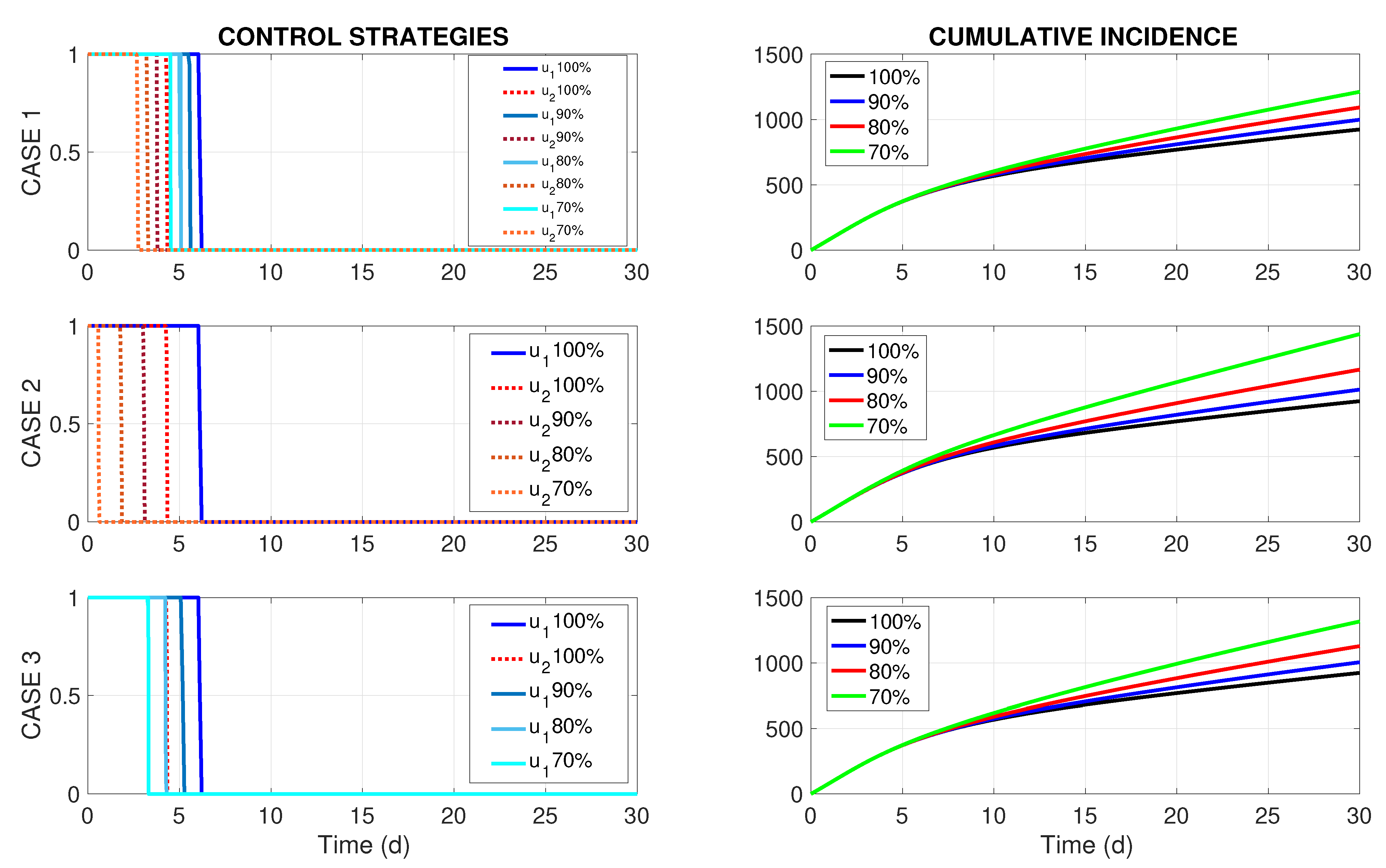
Numerical solutions obtained by GPOPS-II have once again culminated in optimal controls $u_1^{*}\left(t\right),u_2^{*}\left(t\right)$ that are almost identical for all three residence time configurations ${\mathbb{S}}_0,{\mathbb{S}}_1,{\mathbb{S}}_2$. 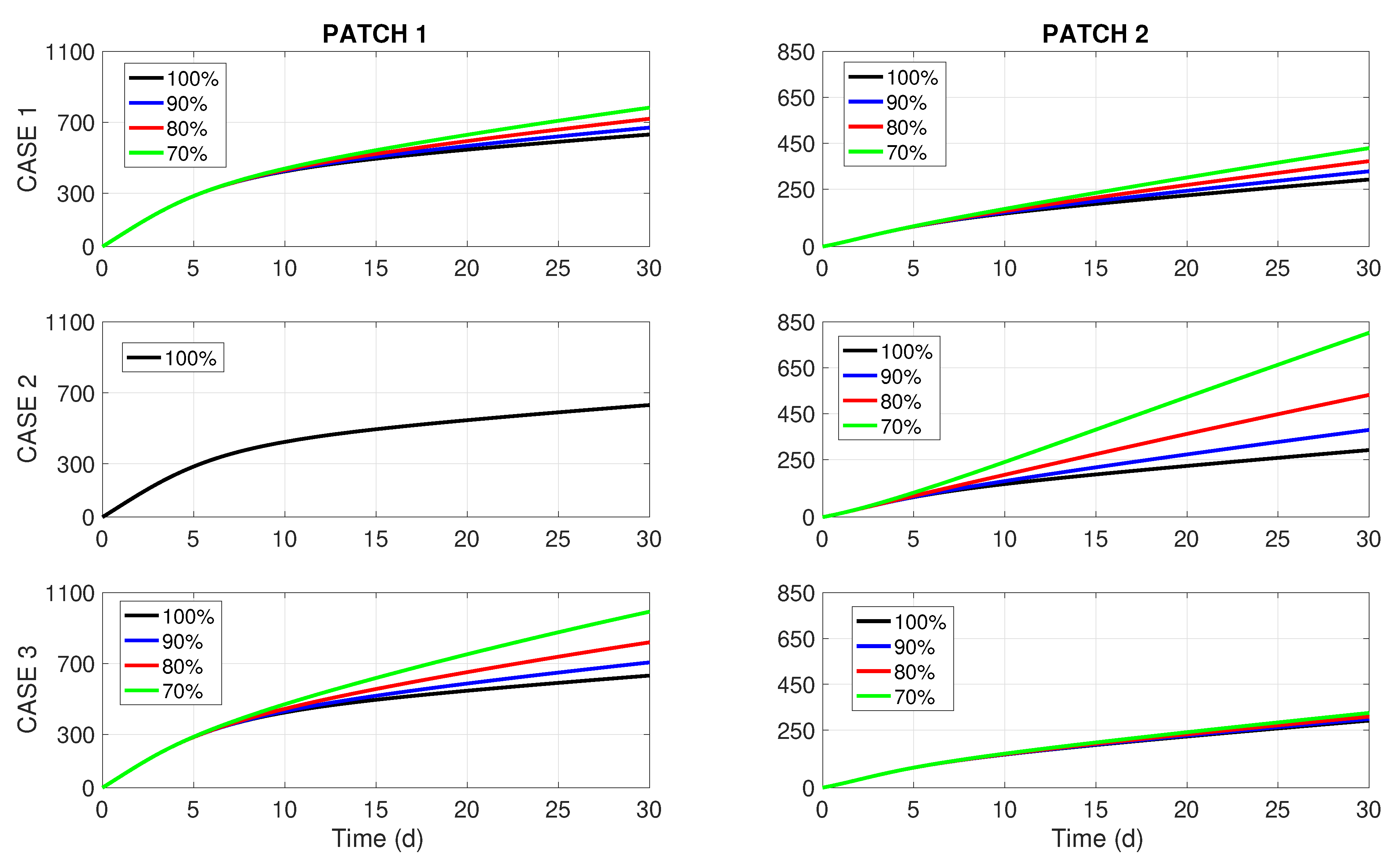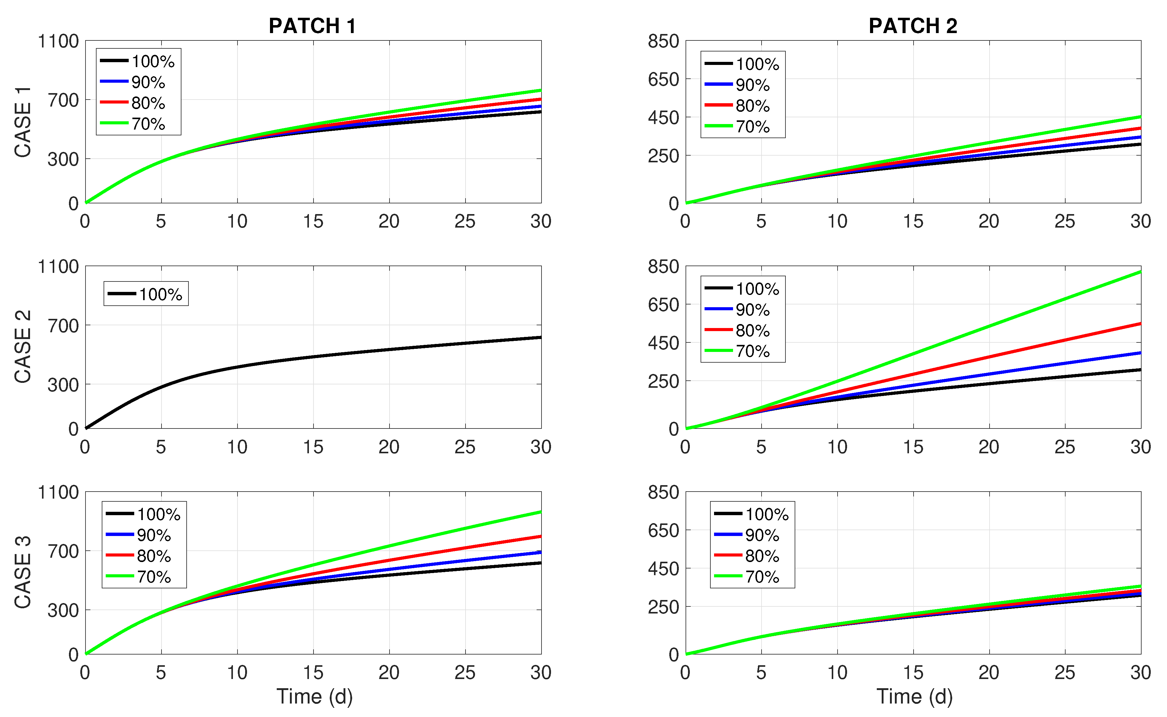The left column of Figure 2 presents the optimal controls $u_1^{*}\left(t\right),u_2^{*}\left(t\right)$ corresponding to the weak coupling (${\mathbb{S}}_1$), while its right column displays the effect of these controls on the total cumulative incidence in both patches. The rows of Figure 2 correspond to Cases 1, 2, and 3 described above. The outcomes for the other two scenarios (uncoupled ${\mathbb{S}}_0$ and with strong coupling ${\mathbb{S}}_2$) look very much like the ones presented in Figure 2, and they are omitted here to save space. Nonetheless, the graphs of $C_{hi}(t;u_1^{*},u_2^{*}), i=1,2$ are presented in Appendix B for all commuting scenarios ${\mathbb{S}}_0,{\mathbb{S}}_1,{\mathbb{S}}_2,$ and the impact of commuting intensity on the number of new disease cases is briefly discussed.

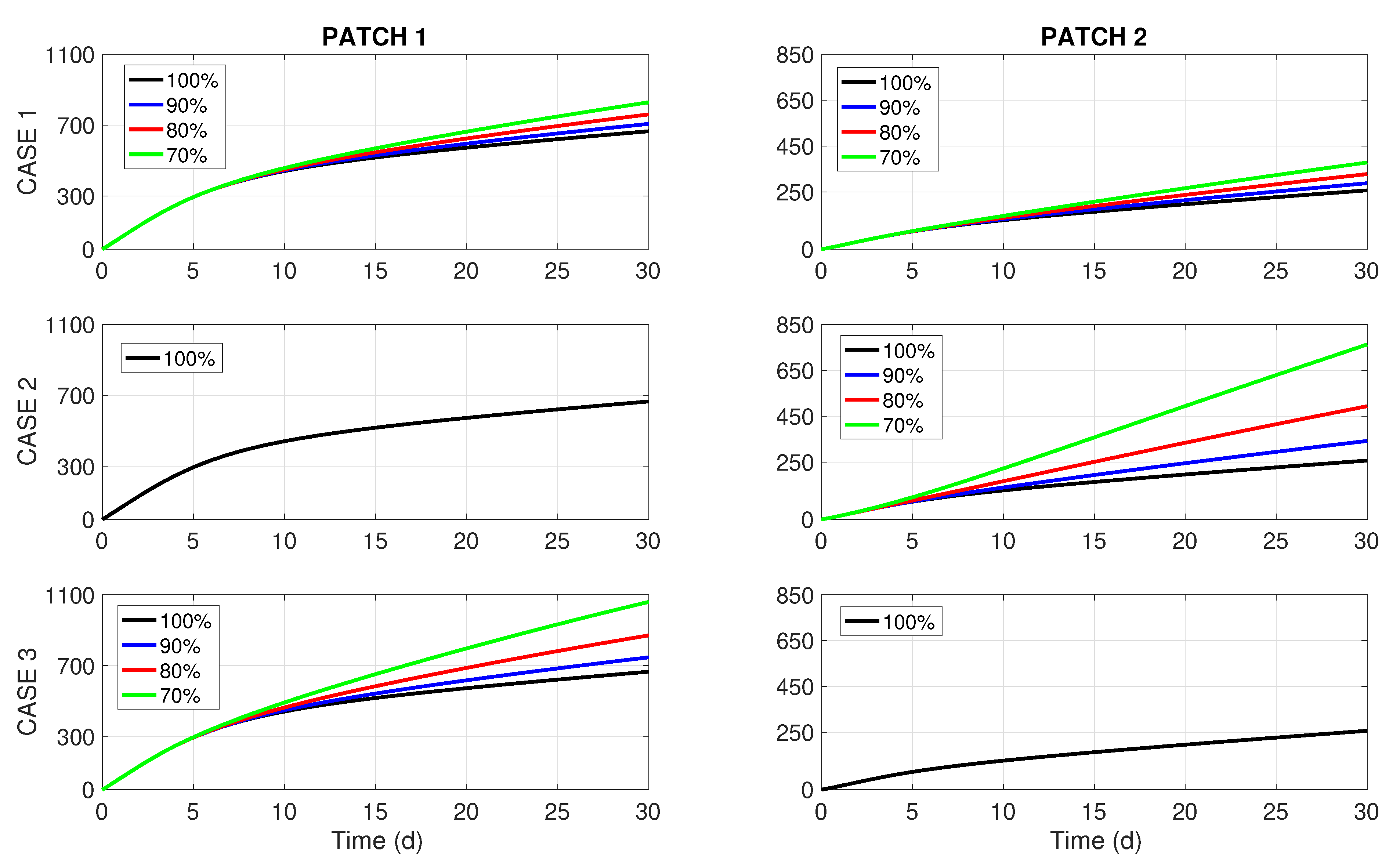
By revising the left column of Figure 2, we notice that the periods of insecticide spraying ($u_i^{*}\left(t\right)=1, i=1,2$) are shortened proportionally to the budget reduction in all Cases 1–3. This feature was also detected in [8], where a more simple one-patch dengue transmission model of the Ross–MacDonald type was studied under resource limitation for insecticide spraying. On the other hand, the right column of Figure 2 brings forward some interesting insights. For a 10% budget cut (i.e., $\sigma =0.9$), we perceive no difference in $C_h(T;u_1^{*},u_2^{*})$ between Cases 1, 2, and 3. However, when the budget cuts become more significant (20% or 30%), it becomes visible that Case 1 (uniform or unbiased distribution of the budget reduction) renders better results than the two biased distributions (Cases 2 and 3). Notably, the most common way of dealing with budget cuts in practice (Case 2, middle chart in the right column of Figure 2) turns out to be the worst choice for dengue control.

In the next section, we bring forward more arguments about the cost of insecticide spraying (with and without budget cuts) and the expenses needed to cure human infections that will still arise after the corrective intervention measures.

4.4. Discussion

Even though dengue-related costs, both direct and indirect, vary significantly across different countries, regions, and socioeconomic contexts, the burden of dengue is often higher in resource-limited settings. Here, the direct costs principally refer to the implementation of vector control measures, both preventive and corrective, and the medical expenses assumed by the local public health units (such as diagnosing and treating dengue cases, including hospitalization, medications, laboratory tests, and specialized care for severe cases). On the other hand, the indirect costs encompass productivity losses by sickness leaves, work absenteeism, and other social consequences such as stress and emotional distress for infected individuals and their families that negatively affect people’s well-being.

In this section, we intend to estimate the direct costs for the three commuting scenarios ${\mathbb{S}}_0,{\mathbb{S}}_1,{\mathbb{S}}_2$ (cf. Table 2) and under three different distributions of budget cuts, described in Section 4.3 as Cases 1, 2, and 3. We will only account for the costs of corrective control measures (insecticide spraying) conducted as an emergency response to suppress the disease outbreak while disregarding the costs of the preventive control measures, which are routinely applied regardless of the disease status. It is worthwhile to point out that the monetary assessment of the indirect costs is a rather challenging task that goes beyond the scope of our study.

The total direct cost related to the dengue outbreak during the observation period of $T=[0,30]$ days will then include the following two components:

• Spending for the insecticide spraying in both patches, expressed by $\sigma B$, where B is defined in (19) and $\sigma \in \left\{0.7,0.8,0.9,1\right\}$ stands for the budget reduction factor.
• Spending for the medical treatment of infected individuals residing in both patches, estimated using the Formulas (17), (18) as $W_1\times C_h(T;u_1^{*},u_2^{*})$, where $u_1^{*}\left(t\right)$ and $u_2^{*}\left(t\right)$ are solutions to the optimal control problem (8) and (9) with budget constraints (21)–(23) obtained for different commuting scenarios ${\mathbb{S}}_0,{\mathbb{S}}_1,{\mathbb{S}}_2$ described in Table 2.

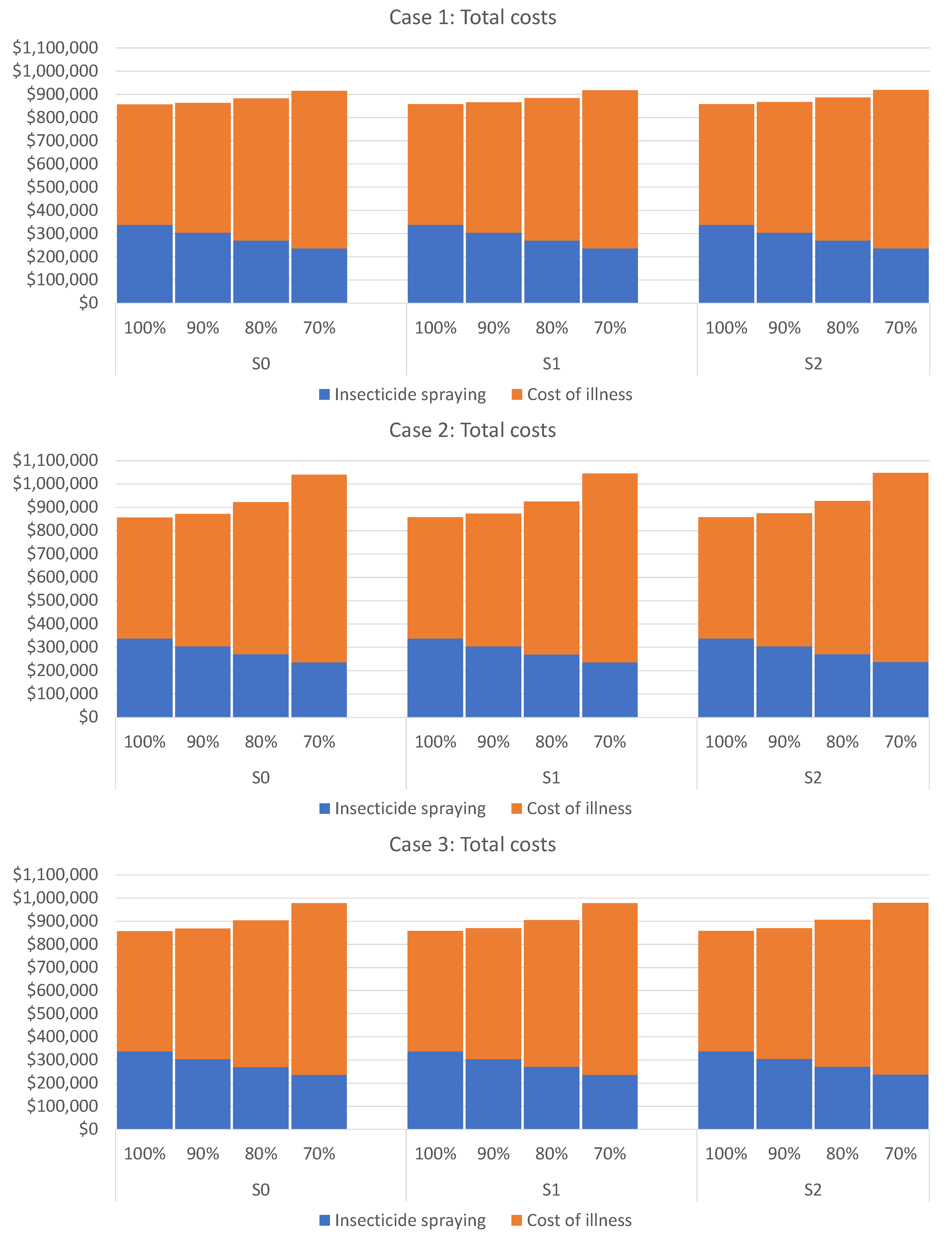
Figure 3 displays the total costs corresponding to Cases 1, 2, and 3 (by rows) under different commuting scenarios ${\mathbb{S}}_0,{\mathbb{S}}_1,$ and ${\mathbb{S}}_2$ (by columns) in the form of bar diagrams. Each bar sums up the two types of spending described above. A cursory glance at the bar diagrams in this figure reveals that cutting the resources for corrective control measures will always lead to a noticeable increase in the total cost. In other words, whatever is “saved” on the insecticide spraying will not suffice to cover the additional medical costs, and the total public spending will increase. Therefore, the best option is not to reduce the funds required for the corrective control measures because their reduction will always induce additional expenses related to illness costs.

Furthermore, we arrive at the following conclusion by comparing the three rows in Figure 3 corresponding to different budget cut distributions (Cases 1–3). If the healthcare authorities only have a fraction $\sigma \in (0,1)$ of the budget $B=B_1+B_2$ required for the corrective control measures, the uniform or unbiased budget reduction seems the most meaningful way to implement them. Moreover, Figure 3 also reveals that the habitual modus operandi for budget reduction (expressed by Case 2) is the most unsuitable option.

Finally, comparing the columns in Figure 3 that correspond to different commuting scenarios ${\mathbb{S}}_0,{\mathbb{S}}_1,$ and ${\mathbb{S}}_2$, we observe no significant differences between them. In other words, the intensity of people commuting does not have a critical impact on the disease spread, at least when the necessary resources for corrective measures are fully available, meaning no budget reduction occurs. The numbers given in Appendix B (see

Table A1. Uncoupled scenario ${\mathbb{S}}_0$: total number of new infections in Patch 1 and Patch 2 expected over 30 days.

Scenario ${\mathbb{S}}_0$		New Infections in 30 Days
		Patch 1	Patch 2	Both
Case 1	100%	666	257	923
	90%	708	288	996
	80%	761	328	1089
	70%	829	378	1207
Case 2	100%	666	257	923
	90%	666	343	1009
	80%	666	494	1160
	70%	666	763	1429
Case 3	100%	666	257	923
	90%	747	257	1004
	80%	871	257	1128
	70%	1060	257	1317

,

Table A2. Weak coupling scenario ${\mathbb{S}}_1$: total number of new infections in Patch 1 and Patch 2 expected over 30 days.

Scenario ${\mathbb{S}}_1$		New Infections in 30 Days
		Patch 1	Patch 2	Both
Case 1	100%	632	292	924
	90%	671	328	999
	80%	720	372	1092
	70%	783	429	1212
Case 2	100%	632	292	924
	90%	633	380	1013
	80%	633	532	1165
	70%	634	803	1437
Case 3	100%	632	292	924
	90%	706	299	1005
	80%	819	309	1128
	70%	992	325	1317

and

Table A3. Strong coupling scenario ${\mathbb{S}}_2$: total number of new infections in Patch 1 and Patch 2 expected over 30 days.

Scenario ${\mathbb{S}}_2$		New Infections in 30 Days
		Patch 1	Patch 2	Both
Case 1	100%	617	308	925
	90%	655	345	1000
	80%	703	392	1095
	70%	763	451	1214
Case 2	100%	617	308	925
	90%	618	396	1014
	80%	619	549	1168
	70%	620	821	1441
Case 3	100%	617	308	925
	90%	688	318	1006
	80%	797	333	1130
	70%	963	356	1319

) indicate that under no budget reduction, a minimal number of expected new infections (merely one or two) can be caused by commuting. Nonetheless, this number increases progressively with the budget reduction.

5. Conclusions

In this paper, we have studied a realistic example of a two-patch dengue transmission model consisting of one big city (Patch 1) and its suburbs (Patch 2) whose residents daily commute to the city for work. It was also assumed that, even though both patches are located in the same dengue-endemic area, the city features lower vectorial density than the suburbs. An epidemic outbreak may occur when the routine preventive measures of vector control do not yield satisfactory results. In such a situation, the local healthcare authorities are compelled to implement urgent insecticide spraying, thus seeking to suppress the number of new infections in humans as quickly as possible. This corrective intervention does not replace the routine preventive measure of vector management because it may harm other non-target living organisms, and it is usually intended only for short-term application.

To design the patch-dependent optimal strategies for corrective control, we formulated an optimal control problem where the objective functional expresses the direct dengue-related costs to be minimized, namely, the costs destined for the insecticide spraying and the public spending for treating dengue infections in humans. Using numerical solutions to the formulated optimal control problem, we showed that the patch-dependent optimal strategies for insecticide spraying have almost no dependency on the intensity of people commuting but their effects significantly depend on the commuting intensity.

Regarding the societal disease-related costs, our approach illustrated that trying “to save money” by reducing the budget for corrective control is entirely unwise. Namely, the anticipated savings on insecticide spraying will further turn into considerable additional public spending for treating human infections, and such extra spending is avoidable by timely corrective intervention.

Furthermore, we have revised a situation when only a share of resources needed to implement the optimal control strategies is available and designed the optimal strategies for both patches under budget constraints. We also considered three different ways of distributing the reduced budget between the two patches. In practice, when there are not enough resources for insecticide spraying in the city and the suburbs, the local healthcare authorities first secure the necessary funds for the control measures in the city, and the rest are used in the suburbs. Our simulation has shown that this habitual modus operandi is the most unwise, for it yields the highest total costs. On the other hand, we have also corroborated that a uniform budget reduction for both patches is the wisest way of acting in resource-limited settings.

Summarizing the outcomes of the present work, we have provided mathematical and computational arguments to support the following recommendations:

• The patch-dependent strategies for corrective vector control can be designed without knowing the intensity of people commuting between the patches. This finding simplifies the design of such strategies because the commuting intensity exhibits variability and uncertainties, while its estimation is complicated and requires additional efforts together with underlying societal costs.
• Saving on corrective vector control measures during the ongoing epidemics is unwise. Such savings will always entail extra spending on disease treatment and enlarge the overall disease-related public expenditures.
• In resource-limited settings, a uniform budget reduction for both patches is the wisest way to distribute the funding because it will produce smaller overall disease-related public expenditures than biased distribution scenarios.

In conclusion, we hope that the outcomes of this study will help in designing patch-dependent strategies for corrective intervention and also send a message to the public healthcare authorities in dengue-endemic countries regarding the necessary adjustments in resource-limited settings.