
Levy Flight and Chaos Theory-Based Gravitational Search Algorithm for Image Segmentation


Abstract
:
1. Introduction
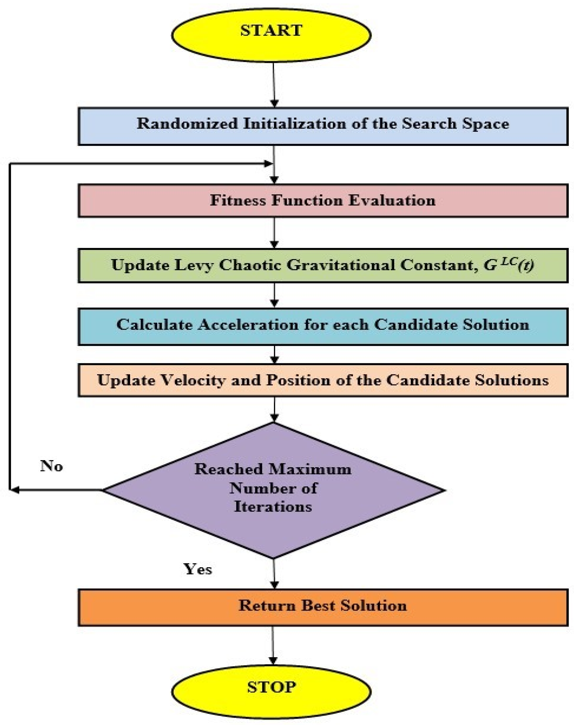
- A novel hybrid image segmentation technique, namely LCGSA, is developed to overcome the inadequacies of traditional segmentation approaches and provide predicted segmented output at a faster speed and reduced processing cost.
- To enhance segmentation results, the algorithm parameters are updated using Levy’s flight and Chaos theory.
- The algorithm incorporates the Levy flight to enhance exploration capabilities and obtain a suitable balance between the exploration and exploitation stages.
- Chaos theory prevents the algorithm from getting trapped in local optima and, hence, increases the chances of locating feasible regions of the search space.
- The proposed LCGSA approach is applied to two benchmark images from the USC-SIPI database.
- Moreover, LCGSA is also applied to three chest CT scan images in order to quickly and efficiently assess the severity of COVID-19 disease.
- An ablation study is carried out on COVID-19 images and infection masks to further authenticate the optimal performance of LCGSA.
- LCGSA’s performance is evaluated and compared with 12 state-of-the-art heuristic algorithms.
2. Literature Survey
3. Methodology
3.1. Gravitational Search Algorithm (GSA)
3.2. Levy Flight and Chaos Theory-Based Gravitational Search Algorithm (LCGSA)
3.2.1. Levy Flight
3.2.2. Chaos Theory
4. Image Segmentation Using LCGSA
5. Experimental Results and Discussion
5.1. Experimental Analysis of Benchmark Images
5.1.1. Simulation Results of the Airport Image
5.1.2. Simulation Results of the Boat Image
5.2. COVID-19 Case Study: Experimental Analysis of COVID-19 CT Scan Images
5.2.1. Simulation Results of the CT1 Image
5.2.2. Simulation Results of the CT2 Image
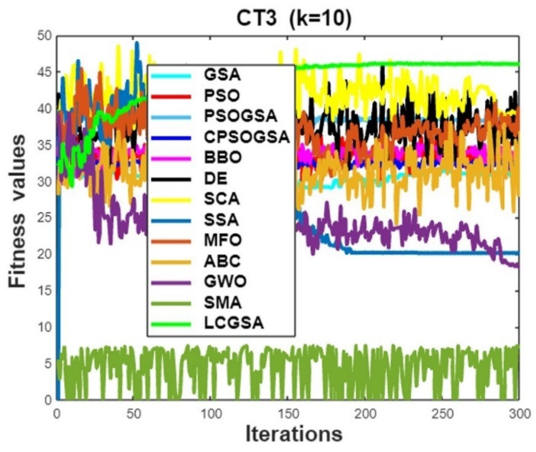
5.2.3. Simulation Results of the CT3 Image
5.3. Statistical Analysis of the Results
6. Ablation Study
6.1. Performance Metrics
6.2. Quantitative and Qualitative Analysis of the Results
6.3. Statistical Analysis of the Results
7. Overall Analysis of Simulation Results
8. Conclusions and Future Scope
Author Contributions
Funding
Data Availability Statement
Conflicts of Interest
Nomenclature
| IS | Image Segmentation |
| MT | Multilevel Thresholding |
| HA | Heuristic Algorithm |
| PSNR | Peak Signal-to-Noise Ratio |
| STD | Standard Deviation |
| SSIM | Structural Similarity Index Measure |
| FSIM | Feature Similarity Index Measure |
| MSE | Mean Square Error |
| BV | Best Value |
| PSO | Particle Swarm Optimization |
| CPSOGSA | Constriction Coefficient-based PSO and GSA |
| GSA | Gravitational Search Algorithm |
| SSA | Salp Swarm Optimizer |
| BBO | Biogeography-Based Optimizer |
| DE | Differentıal Evolution |
| SCA | Sine–Cosine Algorithm |
| MFO | Moth Flame Optimizer |
| ABC | Artificial Bee Colony Algorithm |
| GWO | Gray Wolf Optimizer |
| SMA | Slime Mould Algorithm |
| MIS | Medical Image Segmentation |
References
- Wolpert, D.H.; Macready, W.G. No free lunch theorems for optimization. IEEE Trans. Evol. Comput. 1997, 1, 67–82. [Google Scholar] [CrossRef]
- Alinaghian, M.; Tirkolaee, E.B.; Dezaki, Z.K.; Hejazi, S.R.; Ding, W. An augmented Tabu search algorithm for the green inventory-routing problem with time windows. Swarm Evol. Comput. 2021, 60, 100802. [Google Scholar] [CrossRef]
- Tirkolaee, E.B.; Mardani, A.; Dashtian, Z.; Soltani, M.; Weber, G.-W. A novel hybrid method using fuzzy decision making and multi-objective programming for sustainable-reliable supplier selection in two-echelon supply chain design. J. Clean. Prod. 2020, 250, 119517. [Google Scholar] [CrossRef]
- Bansal, P.; Kumar, S.; Pasrija, S.; Singh, S. A hybrid grasshopper and new cat swarm optimization algorithm for feature selection and optimization of multi-layer perceptron. Soft Comput. 2020, 24, 15463–15489. [Google Scholar] [CrossRef]
- Mirjalili, S. SCA: A Sine Cosine Algorithm for solving optimization problems. Knowl.-Based Syst. 2016, 96, 120–133. [Google Scholar] [CrossRef]
- Mirjalili, S.; Gandomi, A.H.; Mirjalili, S.Z.; Saremi, S.; Faris, H.; Mirjalili, S.M. Salp Swarm Algorithm: A bio-inspired optimizer for engineering design problems. Adv. Eng. Softw. 2017, 114, 163–191. [Google Scholar] [CrossRef]
- Mirjalili, S.; Mirjalili, S.M.; Lewis, A. Grey Wolf Optimizer. Adv. Eng. Softw. 2014, 69, 46–61. [Google Scholar] [CrossRef]
- Erdal, F.; Doğan, E.; Saka, M.P. Optimum design of cellular beams using harmony search and particle swarm optimizers. J. Constr. Steel Res. 2011, 67, 237–247. [Google Scholar] [CrossRef]
- Abualigah, L.; Yousri, D.; Elaziz, M.A.; Ewees, A.A.; Al-Qaness, M.A.; Gandomi, A.H. Aquila Optimizer: A novel meta-heuristic optimization algorithm. Comput. Ind. Eng. 2021, 157, 107250. [Google Scholar] [CrossRef]
- Abualigah, L.; Diabat, A.; Mirjalili, S.; Abd Elaziz, M.; Gandomi, A.H. The arithmetic optimization algo-rithm. Comput. Methods Appl. Mech. Eng. 2021, 376, 113609. [Google Scholar] [CrossRef]
- Ezugwu, A.E.; Agushaka, J.O.; Abualigah, L.; Mirjalili, S.; Gandomi, A.H. Prairie Dog Optimization Algorithm. Neural Comput. Appl. 2022, 34, 20017–20065. [Google Scholar] [CrossRef]
- Agushaka, J.O.; Ezugwu, A.E.; Abualigah, L. Dwarf Mongoose Optimization Algorithm. Comput. Methods Appl. Mech. Eng. 2022, 391, 114570. [Google Scholar] [CrossRef]
- Oyelade, O.N.; Ezugwu, A.E.-S.; Mohamed, T.I.A.; Abualigah, L. Ebola Optimization Search Algorithm: A New Nature-Inspired Metaheuristic Optimization Algorithm. IEEE Access 2022, 10, 16150–16177. [Google Scholar] [CrossRef]
- Abualigah, L.; Abd Elaziz, M.; Sumari, P.; Geem, Z.W.; Gandomi, A.H. Reptile Search Algorithm (RSA): A na-ture-inspired meta-heuristic optimizer. Expert Syst. Appl. 2022, 191, 116158. [Google Scholar] [CrossRef]
- Santos, M.R.; Costa, B.S.J.; Bezerra, C.G.; Andonovski, G.; Guedes, L.A. An evolving approach for fault diagnosis of dynamic systems. Expert Syst. Appl. 2022, 189, 115983. [Google Scholar] [CrossRef]
- Precup, R.-E.; David, R.-C.; Roman, R.-C.; Szedlak-Stinean, A.-I.; Petriu, E.M. Optimal tuning of interval type-2 fuzzy controllers for nonlinear servo systems using Slime Mould Algorithm. Int. J. Syst. Sci. 2021, 1–16. [Google Scholar] [CrossRef]
- Bojan-Dragos, C.-A.; Precup, R.-E.; Preitl, S.; Roman, R.-C.; Hedrea, E.-L.; Szedlak-Stinean, A.-I. GWO-Based Optimal Tuning of Type-1 and Type-2 Fuzzy Controllers for Electromagnetic Actuated Clutch Systems. IFAC-Pap. 2021, 54, 189–194. [Google Scholar] [CrossRef]
- Khurma, R.A.; Aljarah, I.; Sharieh, A.; Mirjalili, S. EvoloPy-FS: An Open-Source Nature-Inspired Optimization Framework in Python for Feature Selection. Evol. Mach. Learn. Tech. Algorithms Appl. 2020, 131–173. [Google Scholar] [CrossRef]
- Karaboga, D. An Idea Based on Honeybee Swarm for Numerical Optimization; Erciyes University: Kayseri, Türkiye, 2005; Volume 200, pp. 1–10. [Google Scholar]
- Mirjalili, S. Moth-flame optimization algorithm: A novel nature-inspired heuristic paradigm. Knowl. Based Syst. 2015, 89, 228–249. [Google Scholar] [CrossRef]
- Kennedy, J.; Eberhart, R. Particle Swarm Optimization. IEEE Int. Conf. Neural Netw. 1995, 4, 1942–1948. [Google Scholar]
- Pereira, J.L.J.; Francisco, M.B.; Diniz, C.A.; Oliver, G.A.; Cunha, S.S.; Gomes, G.F. Lichtenberg algorithm: A novel hybrid physics-based meta-heuristic for global optimization. Expert Syst. Appl. 2021, 170, 114522. [Google Scholar] [CrossRef]
- Erol, O.K.; Eksin, I. A new optimization method: Big Bang–Big Crunch. Adv. Eng. Softw. 2006, 37, 106–111. [Google Scholar] [CrossRef]
- Rashedi, E.; Nezamabadi-Pour, H.; Saryazdi, S. GSA: A Gravitational Search Algorithm. Inf. Sci. 2009, 179, 2232–2248. [Google Scholar] [CrossRef]
- Khalilpourazari, S.; Naderi, B.; Khalilpourazary, S. Multi-Objective Stochastic Fractal Search: A powerful algorithm for solving complex multi-objective optimization problems. Soft Comput. 2020, 24, 3037–3066. [Google Scholar] [CrossRef]
- Holland, J.H. Genetic Algorithms. Sci. Am. 1992, 267, 66–73. [Google Scholar] [CrossRef]
- Ma, H.; Simon, D. Biogeography-based optimization with blended migration for constrained optimization problems. In Proceedings of the 12th Annual Conference on Genetic and Evolutionary Computation, Portland, OR, USA, 7–11 July 2010; pp. 417–418. [Google Scholar] [CrossRef]
- Storn, R.; Price, K. Differential evolution—A simple and efficient heuristic for global optimization over continuous spaces. J. Glob. Optim. 1997, 11, 341–359. [Google Scholar] [CrossRef]
- Wu, F.; Zhao, S.; Yu, B.; Chen, Y.-M.; Wang, W.; Song, Z.-G.; Hu, Y.; Tao, Z.-W.; Tian, J.-H.; Pei, Y.-Y.; et al. A new coronavirus associated with human respiratory disease in China. Nature 2020, 579, 265–269. [Google Scholar] [CrossRef]
- Khalilpourazari, S.; Doulabi, H.H.; Çiftçioğlu, A.; Weber, G.-W. Gradient-based grey wolf optimizer with Gaussian walk: Application in modelling and prediction of the COVID-19 pandemic. Expert Syst. Appl. 2021, 177, 114920. [Google Scholar] [CrossRef]
- Huang, C.; Wang, Y.; Li, X.; Ren, L.; Zhao, J.; Hu, Y.; Zhang, L.; Fan, G.; Xu, J.; Gu, X.; et al. Clinical features of patients infected with 2019 novel coronavirus in Wuhan, China. Lancet 2020, 395, 497–506. [Google Scholar] [CrossRef]
- Chan, J.F.; Yuan, S.; Kok, K.H.; To, K.K.; Chu, H.; Yang, J.; Xing, F.; Liu, J.; Yip, C.C.; Poon, R.W.; et al. A familial cluster of pneumonia associated with the 2019 novel coronavirus indicating person-to-person transmission: A study of a family cluster. Lancet 2020, 395, 514–523. [Google Scholar] [CrossRef]
- World Health Organization. Laboratory Testing for Coronavirus Disease 2019 (COVID-19) in Suspected Human Cases; WHO: Geneva, Switzerland, 2020; pp. 1–7. [Google Scholar]
- Kumar, S.; Sharma, P.P.; Shankar, U.; Kumar, D.; Joshi, S.K.; Pena, L.; Durvasula, R.; Kumar, A.; Kempaiah, P.; Poonam Rathi, B. Discovery of New Hydroxyethylamine Analogs against 3CLpro Protein Target of SARS-CoV-2: Molecular Docking, Molecular Dynamics Simulation, and Structure–Activity Relationship Studies. J. Chem. Inf. Model. 2020, 60, 5754–5770. [Google Scholar] [CrossRef]
- Le, T.T.; Andreadakis, Z.; Kumar, A.; Román, R.G.; Tollefsen, S.; Saville, M.; Mayhew, S. The COVID-19 vaccine development landscape. Nat. Rev. Drug Discov. 2020, 19, 305–306. [Google Scholar] [CrossRef]
- V’kovski, P.; Kratzel, A.; Steiner, S.; Stalder, H.; Thiel, V. Coronavirus biology and replication: Implications for SARS-CoV-2. Nat. Rev. Microbiol. 2021, 19, 155–170. [Google Scholar] [CrossRef]
- Toyoshima, Y.; Nemoto, K.; Matsumoto, S.; Nakamura, Y.; Kiyotani, K. SARS-CoV-2 genomic variations associated with mortality rate of COVID-19. J. Hum. Genet. 2020, 65, 1075–1082. [Google Scholar] [CrossRef] [PubMed]
- Singh, P.; Bose, S.S. A quantum-clustering optimization method for COVID-19 CT scan image segmentation. Expert Syst. Appl. 2021, 185, 115637. [Google Scholar] [CrossRef] [PubMed]
- Munusamy, H.; Muthukumar, K.J.; Gnanaprakasam, S.; Shanmugakani, T.R.; Sekar, A. FractalCovNet architecture for COVID-19 Chest X-ray image Classification and CT-scan image Segmentation. Biocybern. Biomed. Eng. 2021, 41, 1025–1038. [Google Scholar] [CrossRef] [PubMed]
- Feng, H.; Liu, Y.; Lv, M.; Zhong, J. A case report of COVID-19 with false negative RT-PCR test: Necessity of chest CT. Jpn. J. Radiol. 2020, 38, 409–410. [Google Scholar] [CrossRef] [PubMed]
- Ai, T.; Yang, Z.; Hou, H.; Zhan, C.; Chen, C.; Lv, W.; Tao, Q.; Sun, Z.; Xia, L. Correlation of Chest CT and RT-PCR Testing for Coronavirus Disease 2019 (COVID-19) in China: A Report of 1014 Cases. Radiology 2020, 296, E32–E40. [Google Scholar] [CrossRef]
- Sarkar, A.; Vandenhirtz, J.; Nagy, J.; Bacsa, D.; Riley, M. Identification of Images of COVID-19 from Chest X-rays Using Deep Learning: Comparing COGNEX VisionPro Deep Learning 1.0TM Software with Open Source Convolutional Neural Networks. SN Comput. Sci. 2021, 2, 130. [Google Scholar] [CrossRef]
- Liu, L.; Zhao, D.; Yu, F.; Heidari, A.A.; Li, C.; Ouyang, J.; Chen, H.; Mafarja, M.; Turabieh, H.; Pan, J. Ant colony optimization with Cauchy and greedy Levy mutations for multilevel COVID 19 X-ray image segmentation. Comput. Biol. Med. 2021, 136, 104609. [Google Scholar] [CrossRef]
- Wang, G.; Liu, X.; Li, C.; Xu, Z.; Ruan, J.; Zhu, H.; Meng, T.; Li, K.; Huang, N.; Zhang, S. A Noise-Robust Framework for Automatic Segmentation of COVID-19 Pneumonia Lesions from CT Images. IEEE Trans. Med Imaging 2020, 39, 2653–2663. [Google Scholar] [CrossRef] [PubMed]
- Luo, S.; Li, Y.; Gao, P.; Wang, Y.; Serikawa, S. Meta-seg: A survey of meta-learning for image segmentation. Pattern Recognit. 2022, 126, 108586. [Google Scholar] [CrossRef]
- Wang, X.; Li, Z.; Huang, Y.; Jiao, Y. Multimodal medical image segmentation using multi-scale context-aware network. Neurocomputing 2021, 486, 135–146. [Google Scholar] [CrossRef]
- Oskouei, A.G.; Hashemzadeh, M.; Asheghi, B.; Balafar, M.A. CGFFCM: Cluster-weight and Group-local Feature-weight learning in Fuzzy C-Means clustering algorithm for color image segmentation. Appl. Soft Comput. 2021, 113, 108005. [Google Scholar] [CrossRef]
- Civit-Masot, J.; Luna-Perejón, F.; Corral, J.M.R.; Domínguez-Morales, M.; Morgado-Estévez, A.; Civit, A. A study on the use of Edge TPUs for eye fundus image segmentation. Eng. Appl. Artif. Intell. 2021, 104, 104384. [Google Scholar] [CrossRef]
- Fournel, J.; Bartoli, A.; Bendahan, D.; Guye, M.; Bernard, M.; Rauseo, E.; Khanji, M.Y.; Petersen, S.E.; Jacquier, A.; Ghattas, B. Medical image segmentation automatic quality control: A multi-dimensional approach. Med Image Anal. 2021, 74, 102213. [Google Scholar] [CrossRef] [PubMed]
- Cui, X.; Chang, S.; Li, C.; Kong, B.; Tian, L.; Wang, H.; Huang, P.; Yang, M.; Wu, Y.; Li, Z. DEAttack: A differential evolution based attack method for the robustness evaluation of medical image segmentation. Neurocomputing 2021, 465, 38–52. [Google Scholar] [CrossRef]
- Shu, X.; Yang, Y.; Wu, B. A neighbor level set framework minimized with the split Bregman method for medical image segmentation. Signal Process. 2021, 189, 108293. [Google Scholar] [CrossRef]
- Cai, Y.; Mi, S.; Yan, J.; Peng, H.; Luo, X.; Yang, Q.; Wang, J. An unsupervised segmentation method based on dynamic threshold neural P systems for color images. Inf. Sci. 2022, 587, 473–484. [Google Scholar] [CrossRef]
- Chen, X.; Huang, H.; Heidari, A.A.; Sun, C.; Lv, Y.; Gui, W.; Liang, G.; Gu, Z.; Chen, H.; Li, C.; et al. An efficient multilevel thresholding image segmentation method based on the slime mould algorithm with bee foraging mechanism: A real case with lupus nephritis images. Comput. Biol. Med. 2021, 142, 105179. [Google Scholar] [CrossRef]
- Dai, M.; Baylou, P.; Humbert, L.; Najim, M. Image segmentation by a dynamic thresholding using edge detection based on cascaded uniform filters. Signal Process. 1996, 52, 49–63. [Google Scholar] [CrossRef]
- Chakraborty, S.; Mali, K. Biomedical image segmentation using fuzzy multilevel soft thresholding system coupled modified cuckoo search. Biomed. Signal Process. Control. 2022, 72, 103324. [Google Scholar] [CrossRef]
- Wu, T.; Shao, J.; Gu, X.; Ng, M.K.; Zeng, T. Two-stage image segmentation based on nonconvex ℓ2−ℓp approximation and thresholding. Appl. Math. Comput. 2021, 403, 126168. [Google Scholar] [CrossRef]
- Kalyani, R.; Sathya, P.; Sakthivel, V. Trading strategies for image segmentation using multilevel thresholding aided with minimum cross entropy. Eng. Sci. Technol. Int. J. 2020, 23, 1327–1341. [Google Scholar] [CrossRef]
- Abdel-Basset, M.; Mohamed, R.; AbdelAziz, N.M.; Abouhawwash, M. HWOA: A hybrid whale optimization algorithm with a novel local minima avoidance method for multi-level thresholding color image segmentation. Expert Syst. Appl. 2022, 190, 116145. [Google Scholar] [CrossRef]
- Houssein, E.H.; Hussain, K.; Abualigah, L.; Elaziz, M.A.; Alomoush, W.; Dhiman, G.; Djenouri, Y.; Cuevas, E. An improved opposition-based marine predators algorithm for global optimization and multilevel thresholding image segmentation. Knowl.-Based Syst. 2021, 229, 107348. [Google Scholar] [CrossRef]
- Zhao, D.; Liu, L.; Yu, F.; Heidari, A.A.; Wang, M.; Oliva, D.; Muhammad, K.; Chen, H. Ant colony optimization with horizontal and vertical crossover search: Fundamental visions for multi-threshold image segmentation. Expert Syst. Appl. 2021, 167, 114122. [Google Scholar] [CrossRef]
- Cao, X.; Li, T.; Li, H.; Xia, S.; Ren, F.; Sun, Y.; Xu, X. A Robust Parameter-Free Thresholding Method for Image Segmentation. IEEE Access 2019, 7, 3448–3458. [Google Scholar] [CrossRef]
- Bhandari, A.K.; Kumar, A.; Singh, G.K. Modified artificial bee colony based computationally efficient multilevel thresholding for satellite image segmentation using Kapur’s, Otsu and Tsallis functions. Expert Syst. Appl. 2015, 42, 1573–1601. [Google Scholar] [CrossRef]
- Kotte, S.; Kumar, P.R.; Injeti, S.K. An efficient approach for optimal multilevel thresholding selection for gray scale images based on improved differential search algorithm. Ain Shams Eng. J. 2018, 9, 1043–1067. [Google Scholar] [CrossRef]
- Khalilpourazari, S.; Pasandideh, S.H.R. Modeling and optimization of multi-item multi-constrained EOQ model for growing items. Knowl.-Based Syst. 2019, 164, 150–162. [Google Scholar] [CrossRef]
- Rather, S.A.; Bala, P.S. Swarm-based chaotic gravitational search algorithm for solving mechanical engineering design problems. World J. Eng. 2020, 17, 97–114. [Google Scholar] [CrossRef]
- Rather, S.A.; Bala, P.S. Analysis of Gravitation-Based Optimization Algorithms for Clustering and Classification. In Handbook of Research on Big Data Clustering and Machine Learning; IGI Global: Hershey, PA, USA, 2020; pp. 74–99. [Google Scholar] [CrossRef]
- Rather, S.A.; Bala, P.S. Hybridization of Constriction Coefficient Based Particle Swarm Optimization and Gravitational Search Algorithm for Function Optimization. In Proceedings of the International Conference on Advances in Electronics, Electrical & Computational Intelligence (ICAEEC), Prayagraj, India, 31 May–1 June 2019. [Google Scholar]
- Kandhway, P.; Bhandari, A.K. A Water Cycle Algorithm-Based Multilevel Thresholding System for Color Image Segmentation Using Masi Entropy. Circuits Syst. Signal Process. 2019, 38, 3058–3106. [Google Scholar] [CrossRef]
- Jamazi, C.; Manita, G.; Chhabra, A.; Manita, H.; Korbaa, O. Mutated Aquila Optimizer for assisting brain tumor segmentation. Biomed. Signal Process. Control. 2023, 105089. [Google Scholar] [CrossRef]
- Abualigah, L.; Diabat, A.; Sumari, P.; Gandomi, A. A Novel Evolutionary Arithmetic Optimization Algorithm for Multilevel Thresholding Segmentation of COVID-19 CT Images. Processes 2021, 9, 1155. [Google Scholar] [CrossRef]
- Abualigah, L.; Habash, M.; Hanandeh, E.S.; Hussein, A.M.; Al Shinwan, M.; Abu Zitar, R.; Jia, H. Improved Reptile Search Algorithm by Salp Swarm Algorithm for Medical Image Segmentation. J. Bionic Eng. 2023, 20, 1766–1790. [Google Scholar] [CrossRef]
- Su, H.; Zhao, D.; Yu, F.; Heidari, A.A.; Zhang, Y.; Chen, H.; Li, C.; Pan, J.; Quan, S. Horizontal and vertical search artificial bee colony for image segmentation of COVID-19 X-ray images. Comput. Biol. Med. 2022, 142, 105181. [Google Scholar] [CrossRef] [PubMed]
- Chakraborty, S.; Saha, A.K.; Nama, S.; Debnath, S. COVID-19 X-ray image segmentation by modified whale optimization algorithm with population reduction. Comput. Biol. Med. 2021, 139, 104984. [Google Scholar] [CrossRef] [PubMed]
- Zhang, Q.; Wang, Z.; Heidari, A.A.; Gui, W.; Shao, Q.; Chen, H.; Zaguia, A.; Turabieh, H.; Chen, M. Gaussian Barebone Salp Swarm Algorithm with Stochastic Fractal Search for medical image segmentation: A COVID-19 case study. Comput. Biol. Med. 2021, 139, 104941. [Google Scholar] [CrossRef] [PubMed]
- Houssein, E.H.; Helmy, B.E.; Oliva, D.; Jangir, P.; Premkumar, M.; Elngar, A.A.; Shaban, H. An efficient mul-ti-thresholding based COVID-19 CT images segmentation approach using an improved equilibrium optimizer. Biomed. Signal Process. Control 2022, 73, 103401. [Google Scholar] [CrossRef]
- Zhao, C.; Xu, Y.; He, Z.; Tang, J.; Zhang, Y.; Han, J.; Shi, Y.; Zhou, W. Lung segmentation and automatic detection of COVID-19 using radiomic features from chest CT images. Pattern Recognit. 2021, 119, 108071. [Google Scholar] [CrossRef] [PubMed]
- Jin, Q.; Cui, H.; Sun, C.; Meng, Z.; Wei, L.; Su, R. Domain adaptation based self-correction model for COVID-19 infection segmentation in CT images. Expert Syst. Appl. 2021, 176, 114848. [Google Scholar] [CrossRef] [PubMed]
- Nama, S. A novel improved SMA with quasi reflection operator: Performance analysis, application to the image seg-mentation problem of COVID-19 chest X-ray images. Appl. Soft Comput. 2022, 118, 108483. [Google Scholar] [CrossRef]
- Dimitrov, D.; Abdo, H. Tight independent set neighborhood union condition for fractional critical deleted graphs and ID deleted graphs. Discret. Contin. Dyn. Syst.-S 2018, 12, 711. [Google Scholar] [CrossRef]
- Gao, W.; Guirao, J.L.; Basavanagoud, B.; Wu, J. Partial multi-dividing ontology learning algorithm. Inf. Sci. 2018, 467, 35–58. [Google Scholar] [CrossRef]
- Jensi, R.; Jiji, G.W. An enhanced particle swarm optimization with levy flight for global optimization. Appl. Soft Comput. 2016, 43, 248–261. [Google Scholar] [CrossRef]
- Li, Y.; Li, X.; Liu, J.; Ruan, X. An improved bat algorithm based on lévy flights and adjustment factors. Symmetry 2019, 11, 925. [Google Scholar] [CrossRef]
- Mandelbrot, B.B. The Fractal Geometry of Nature; WH Freeman: New York, NY, USA, 1982. [Google Scholar]
- Yang, X.-S. Chapter 3-Random Walks and Optimization. In Nature-Inspired Optimization Algorithms; Yang, X.-S., Ed.; Elsevier: Oxford, UK, 2014; pp. 45–65. [Google Scholar]
- Gutowski, M. Levy Flights as an underlying mechanism for global optimization algorithms. arXiv 2001, arXiv:0106003. [Google Scholar]
- Pavlyukevich, I. Lévy flights, non-local search and simulated annealing. J. Comput. Phys. 2007, 226, 1830–1844. [Google Scholar] [CrossRef]
- Ramos-Fernández, G.; Mateos, J.L.; Miramontes, O.; Cocho, G.; Larralde, H.; Ayala-Orozco, B. Levy walk patterns in the foraging movements of spider monkeys (Ateles geoffroyi). Behav. Ecol. Sociobiol. 2004, 55, 223–230. [Google Scholar]
- Mirjalili, S.; Gandomi, A.H. Chaotic gravitational constants for the gravitational search algorithm. Appl. Soft Comput. J. 2017, 53, 407–419. [Google Scholar] [CrossRef]
- Alatas, B. Chaotic bee colony algorithms for global numerical optimization. Expert Syst. Appl. 2010, 37, 5682–5687. [Google Scholar] [CrossRef]
- Li, C.; Zhou, J.; Xiao, J.; Xiao, H. Parameters identification of chaotic system by chaotic gravitational search algorithm. Chaos Solitons Fractals 2012, 45, 539–547. [Google Scholar] [CrossRef]
- Mingjun, J.; Huanwen, T. Application of chaos in simulated annealing. Chaos Solitons Fractals 2004, 21, 933–941. [Google Scholar] [CrossRef]
- Gandomi, A.H.; Yang, X.-S.; Talatahari, S.; Alavi, A.H. Firefly algorithm with chaos. Commun. Nonlinear Sci. Numer. Simul. 2013, 18, 89–98. [Google Scholar] [CrossRef]
- Wang, N.; Liu, L.; Liu, L. Genetic algorithm in chaos. OR Trans. 2001, 5, 1–10. [Google Scholar]
- Li-Jiang, Y.; Tian-Lun, C. Application of Chaos in Genetic Algorithms. Commun. Theor. Phys. 2002, 38, 168–172. [Google Scholar] [CrossRef]
- Jothiprakash, V.; Arunkumar, R. Optimization of Hydropower Reservoir Using Evolutionary Algorithms Coupled with Chaos. Water Resour. Manag. 2013, 27, 1963–1979. [Google Scholar] [CrossRef]
- Zhenyu, G.; Bo, C.; Min, Y.; Binggang, C. Self-Adaptive Chaos Differential Evolution. In Advances in Natural Computation: Second International Conference ICNC, Xi’an, China, 24–28 September 2006; Springer: Berlin/Heidelberg, German, 2006; pp. 972–975. [Google Scholar]
- Saremi, S.; Mirjalili, S.M.; Mirjalili, S. Chaotic Krill Herd Optimization Algorithm. Procedia Technol. 2014, 12, 180–185. [Google Scholar] [CrossRef]
- Wang, G.-G.; Guo, L.; Gandomi, A.H.; Hao, G.-S.; Wang, H. Chaotic Krill Herd algorithm. Inf. Sci. 2014, 274, 17–34. [Google Scholar] [CrossRef]
- Peitgen, H.; Jurgens, H.; Saupes, D. Chaos and Fractals; Springer: New York, NY, USA, 1992. [Google Scholar]
- Li, Y.; Deng, S.; Xiao, D. A novel Hash algorithm construction based on chaotic neural network. Neural Comput. Appl. 2011, 20, 133–141. [Google Scholar] [CrossRef]
- Ott, E. Chaos in Dynamical Systems; Cambridge University Press: Cambridge, UK, 2002. [Google Scholar]
- Zhao, S.; Wang, P.; Heidari, A.A.; Chen, H.; Turabieh, H.; Mafarja, M.; Li, C. Multilevel threshold image seg-mentation with diffusion association slime mould algorithm and Renyi’s entropy for chronic obstructive pulmonary disease. Comput. Biol. Med. 2021, 134, 104427. [Google Scholar] [CrossRef] [PubMed]
- Derrac, J.; García, S.; Molina, D.; Herrera, F. A practical tutorial on the use of nonparametric statistical tests as a methodology for comparing evolutionary and swarm intelligence algorithms. Swarm Evol. Comput. 2011, 1, 3–18. [Google Scholar] [CrossRef]
- Wilcoxon, F. Individual Comparisons by Ranking Methods. Biom. Bull. 1945, 1, 80. [Google Scholar] [CrossRef]


| Reference | Algorithm Used | Thresholding Technique | Performance | Comparative Algorithms | Performance Metrics |
|---|---|---|---|---|---|
| Abualigah et al., 2023 [71] | RSA-SSA | Otsu’s variance scheme | Improved segmentation of COVID-19 images and reduction in computational overhead | AO, WOA, SSA, RSA, MPA, and PSO | SSIM, PSNR, Best Fitness values, and statistical tests |
| Jamazi et al., 2023 [69] | AO | K-means | Improved brain tumor detection | Fuzzy C-means, U-Net, Z-Net, Adaptive K-means, SegNet, and so on | PSNR, SSIM, MSE, DSC (Dice Similarity Coefficient), and Sensitivity |
| Su et al., 2022 [72] | CCABC | Kapur entropy | Improved performance with high threshold values | ABC, SCA, MFO, PSO, SSA, CBA, ACWOA, IWOA, IGWO, and HHO | PSNR, SSIM, and FSIM |
| Nama, 2022 [78] | QRSMA | Shannon entropy | Improved accuracy and convergence speed | SMA, MFO, SCA, SHO, SOA, STOA, TSA, and WOA | MSE and PSNR |
| Houssein et al., 2022 [75] | I-EO | Fuzzy entropy | Increased accuracy, PSNR, SSIM, and FSIM | AGDE, GWO, MFO, SCA, HHO, and TSA | PSNR, SSIM, and FSIM |
| Abualigah et al., 2021 [70] | AOA | Kapur entropy | Improved quality of segmentation | AO, WOA, SSA, PSO, MPA, and DE | PSNR, SSIM, and Optimal threshold values |
| Chakraborty et al., 2021 [73] | mWOAPR | Kapur entropy | Enhanced performance | WOA, HBO, HGS, SMA, and variant algorithms of WOA | PSNR and SSIM |
| Liu et al., 2021 [43] | CLACO | Kapur entropy | Improved performance of search capability and convergence speed | GWO, MFO, PSO, ACOR (ant colony optimization (ACO) for continuous domains), SCA, WOA, OBLGWO (boosted GWO), mSCA (modified SCA), and OBSCA (opposition-based SCA) | PSNR, SSIM, and FSIM |
| Singh et al., 2021 [38] | FFQOAK | Euclidean distance | Improved MSE, PSNR, and JSC | GAK, PSOK, DPSOK, and ACOK | MSE, PSNR, Jaccard Similarity Coefficient (JSC), and MSE |
| Zhang et al., 2021 [74] | GBSFSSSA | Kapur entropy | Improved performance of medical image segmentation, search capability, and convergence speed | PSO, SCA, BA, FA, MFO, WOA, and HHO | PSNR, SSIM, and FSIM |
| Zhao et al., 2021 [76] | SP-V-Net | Sigmoid cross-entropy | Improved accuracy, sensitivity, and accelerated convergence | MC-V-Net (multi-channel V-Net) and V-Net | Optimal segmentation |
| Munusamy et al., 2021 [39] | FractalCovNet | Cross-entropy | Improved accuracy, precision, and recall | U-Net, DenseUNet, Segnet, FCN, ResnetUNet, ResNet5, Xception, Inception- ResNetV2, and VGG-16 | F-measure and Dice Coefficient |
| Jin et al., 2021 [77] | DASC-Net | Cross-entropy | Improved segmentation | U-Net, U2-Net, AdaptSegNet, and ADVENT | Sensitivity, Specificity, Jaccard, and Dice Coefficient |
| Kandhway et al., 2019 [68] | WCA | Masi/Tsallis entropies | Convergence speed | BAT, PSO, WDO, MBO, and GOA | PSNR, MSE, FSIM, and SSIM |
| Proposed method | LCGSA | Kapur entropy | To enhance segmentation and resolve computational issues | GSA, PSO, PSOGSA, CPSOGSA, SCA, SSA, BBO, and so on | PSNR, SSIM, MSE, FSIM, BV, STD, and so on |
| Algorithm | k | Optimal Thresholds | Mean | STD | MSE | PSNR | SSIM | FSIM | Best Value | Run Time |
|---|---|---|---|---|---|---|---|---|---|---|
| 2 | 121, 136 | 15.94 | 0.78 | 4898.26 | 11.23 | 0.23 | 0.75 | 16.76 | 4.8409 | |
| 4 | 71, 89, 118, 158 | 17.22 | 0.09 | 1718.12 | 15.78 | 0.60 | 0.88 | 20.31 | 13.3771 | |
| GSA | 6 | 197, 206, 147, 221, 176, 205 | 17.82 | 0.32 | 6441.58 | 10.04 | 0.11 | 0.67 | 28.75 | 11.7766 |
| 8 | 160, 163, 125, 156, 180, 194, 141, 160 | 27.89 | 0.52 | 5093.27 | 11.06 | 0.22 | 0.73 | 33.36 | 19.1112 | |
| 10 | 125, 177, 187, 204, 133, 191, 174, 183, 190, 210 | 35.39 | 0.25 | 5103.71 | 11.05 | 0.22 | 0.74 | 37.03 | 19.6661 | |
| 2 | 7, 21 | 0.44 | 0.41 | 5101.20 | 11.05 | 0.20 | 0.43 | 8.41 | 4.6734 | |
| 4 | 5, 17, 26, 29 | 10.50 | 0.65 | 4173.27 | 11.92 | 0.25 | 0.43 | 15.45 | 11.6513 | |
| PSO | 6 | 22, 36, 54, 81, 59, 76 | 23.32 | 0.92 | 933.84 | 18.42 | 0.71 | 0.75 | 23.85 | 1.4316 |
| 8 | 16, 22, 25, 46, 72, 76, 77, 114 | 27.54 | 1.11 | 479.48 | 21.32 | 0.89 | 0.91 | 28.81 | 15.5366 | |
| 10 | 8, 18, 29, 32, 33, 77, 103, 90, 69, 93 | 29.16 | 1.18 | 684.62 | 19.77 | 0.82 | 0.85 | 33.80 | 17.4482 | |
| 2 | 12, 15 | 8.35 | 0.51 | 5881.14 | 10.43 | 0.15 | 0.42 | 9.75 | 4.1786 | |
| 4 | 17, 39, 70, 74 | 0.37 | 0.47 | 1303.79 | 16.97 | 0.66 | 0.73 | 16.56 | 10.9052 | |
| PSOGSA | 6 | 14, 23, 31, 34, 36, 51 | 22.72 | 0.89 | 2231.51 | 14.64 | 0.40 | 0.55 | 24.75 | 9.0639 |
| 8 | 1, 6, 21, 33, 64, 69, 93, 106 | 19.72 | 0.41 | 593.23 | 20.39 | 0.85 | 0.87 | 31.88 | 12.3254 | |
| 10 | 1, 51, 55, 68, 79, 85, 97, 107, 128, 134 | 30.09 | 0.45 | 502.64 | 21.11 | 0.84 | 0.90 | 34.56 | 15.9034 | |
| 2 | 6, 22 | 8.15 | 0.39 | 4978.21 | 11.16 | 0.21 | 0.43 | 10.65 | 4.5809 | |
| 4 | 7, 7, 34, 52 | 13.75 | 0.53 | 2183.65 | 14.73 | 0.42 | 0.57 | 16.76 | 11.5291 | |
| CPSOGSA | 6 | 25, 32, 36, 60, 102, 111 | 16.03 | 0.24 | 555.38 | 20.68 | 0.88 | 0.89 | 26.32 | 9.1880 |
| 8 | 7, 10, 32, 36, 57, 60, 61, 63 | 17.89 | 0.97 | 1663.74 | 15.91 | 0.52 | 0.64 | 30.69 | 14.0344 | |
| 10 | 2, 14, 22, 29, 31, 48, 64, 101, 109, 114 | 31.47 | 0.43 | 414.51 | 21.95 | 0.90 | 0.90 | 34.37 | 15.9678 | |
| 2 | 118, 79 | 8.12 | 0.97 | 2371.67 | 14.38 | 0.52 | 0.86 | 16.93 | 6.0754 | |
| 4 | 146, 94, 44, 220 | 16.49 | 0.72 | 654.73 | 19.97 | 0.87 | 0.92 | 20.55 | 11.2251 | |
| BBO | 6 | 63, 194, 59, 33, 215, 146 | 18.29 | 0.82 | 969.47 | 18.26 | 0.78 | 0.83 | 25.16 | 15.9688 |
| 8 | 82, 24, 255, 105, 198, 198, 134, 37 | 19.81 | 0.89 | 495.16 | 21.18 | 0.90 | 0.94 | 32.62 | 21.9184 | |
| 10 | 185, 203, 92, 230, 123, 238, 120, 5, 77, 93 | 39.99 | 1.11 | 1698.75 | 15.82 | 0.63 | 0.89 | 44.87 | 23.9526 | |
| 2 | 250, 106 | 12.51 | 1.85 | 3899.23 | 12.22 | 0.32 | 0.80 | 16.92 | 6.3959 | |
| 4 | 227, 59, 235, 150 | 20.81 | 1.60 | 1907.83 | 15.32 | 0.60 | 0.81 | 23.51 | 11.1228 | |
| DE | 6 | 43, 141, 88, 41, 167, 218 | 26.01 | 2.18 | 568.21 | 20.58 | 0.89 | 0.93 | 29.98 | 15.9738 |
| 8 | 225, 196, 194, 140, 61, 250, 157, 17 | 30.10 | 2.42 | 1241.34 | 17.19 | 0.75 | 0.87 | 36.64 | 22.2046 | |
| 10 | 117, 40, 188, 219, 137, 39, 41, 21, 74, 7 | 34.98 | 2.68 | 369.53 | 22.45 | 0.93 | 0.95 | 44.05 | 23.7699 | |
| 2 | 7, 143 | 9.97 | 1.63 | 2239.37 | 14.62 | 0.55 | 0.87 | 17.25 | 5.6035 | |
| 4 | 79, 132, 151, 3 | 18.86 | 1.79 | 2218.69 | 14.66 | 0.56 | 0.89 | 24.43 | 14.3033 | |
| SCA | 6 | 108, 157, 37, 240, 8, 59 | 28.67 | 2.56 | 471.57 | 21.39 | 0.91 | 0.94 | 31.14 | 13.8524 |
| 8 | 24, 8, 133, 166, 248, 40, 118, 174 | 30.47 | 2.81 | 1145.66 | 17.54 | 0.76 | 0.82 | 39.38 | 22.8713 | |
| 10 | 178, 26, 50, 2, 70, 84, 188, 37, 66, 194 | 40.33 | 3.26 | 539.14 | 20.81 | 0.84 | 0.85 | 47.54 | 21.6741 | |
| 2 | 25, 1 | 9.97 | 3.97 | 4621.25 | 11.48 | 0.23 | 0.43 | 12.59 | 5.1492 | |
| 4 | 97, 22, 131, 99 | 17.41 | 1.95 | 1585.80 | 16.12 | 0.71 | 0.87 | 18.27 | 14.1512 | |
| SSA | 6 | 206, 215, 255, 1, 253, 255 | 14.52 | 3.19 | 7613.13 | 9.31 | 0.03 | 0.49 | 25.64 | 13.2537 |
| 8 | 255, 54, 255, 255, 254, 205, 255, 2 | 29.62 | 3.84 | 2285.54 | 14.54 | 0.46 | 0.66 | 29.24 | 24.3640 | |
| 10 | 255, 255, 255, 255, 133, 115, 228, 255, 255, 255 | 31.68 | 9.63 | 4426.80 | 11.66 | 0.28 | 0.77 | 34.27 | 21.0928 | |
| 2 | 255, 1 | 13.62 | 1.46 | 7981.00 | 9.11 | 0.01 | 0.40 | 15.72 | 3.9914 | |
| 4 | 255, 240, 1, 1 | 10.71 | 5.91 | 7981.00 | 9.11 | 0.01 | 0.40 | 19.74 | 6.3647 | |
| MFO | 6 | 1, 2, 255, 1, 255, 1 | 19.96 | 3.58 | 7981.00 | 9.11 | 0.01 | 0.40 | 25.88 | 8.5121 |
| 8 | 254, 1, 2, 1, 255, 254, 255, 1 | 30.81 | 2.81 | 7818.01 | 9.19 | 0.02 | 0.41 | 26.26 | 10.8618 | |
| 10 | 254, 255, 255, 141, 1, 255, 225, 255, 1, 254 | 31.23 | 5.67 | 6075.18 | 10.29 | 0.15 | 0.70 | 36.00 | 13.6318 | |
| 2 | 213, 229 | 12.73 | 1.94 | 7870.28 | 9.17 | 0.01 | 0.49 | 14.32 | 10.2643 | |
| 4 | 153, 192, 193, 214 | 17.38 | 2.09 | 6647.10 | 9.90 | 0.09 | 0.65 | 20.28 | 17.4111 | |
| ABC | 6 | 196, 249, 152, 215, 243, 175 | 21.97 | 2.24 | 6605.16 | 9.93 | 0.10 | 0.65 | 27.35 | 24.8882 |
| 8 | 183, 180, 201, 184, 211, 220, 232, 164 | 26.78 | 2.33 | 6955.69 | 9.70 | 0.07 | 0.60 | 31.71 | 30.8205 | |
| 10 | 212, 235, 242, 226, 238, 204, 225, 187, 228, 185 | 27.34 | 2.86 | 7371.75 | 9.45 | 0.04 | 0.54 | 32.58 | 37.8003 | |
| 2 | 33, 40 | 13.23 | 1.26 | 3022.12 | 13.32 | 0.31 | 0.44 | 11.26 | 3.0042 | |
| 4 | 75, 83, 82, 2 | 18.96 | 1.83 | 2524.06 | 14.10 | 0.48 | 0.78 | 14.84 | 5.5414 | |
| GWO | 6 | 3, 4, 0, 0, 0, 7 | 6.50 | 4.93 | 7033.06 | 9.65 | 0.07 | 0.42 | 14.08 | 8.0195 |
| 8 | 0, 32, 9, 1, 25, 0, 0, 1 | 12.06 | 7.25 | 3757.31 | 0.27 | 0.44 | 0.43 | 14.55 | 9.9017 | |
| 10 | 0, 1, 2, 0, 0, 0, 1, 5, 3, 0 | 0.80 | 4.58 | 7981.00 | 9.11 | 0.01 | 0.40 | 8.16 | 12.9664 | |
| 2 | 144, 140 | 4.73 | 2.33 | 6373.53 | 10.08 | 0.11 | 0.69 | 6.66 | 3.5162 | |
| 4 | 200, 201, 180, 190 | 4.90 | 2.37 | 7692.86 | 9.26 | 0.02 | 0.50 | 6.80 | 5.8604 | |
| SMA | 6 | 1, 1, 1, 2, 5, 10 | 4.59 | 2.44 | 7981.00 | 9.11 | 0.01 | 0.40 | 6.77 | 8.4221 |
| 8 | 197, 191, 189, 188, 190, 178, 197, 197 | 4.79 | 2.32 | 7621.13 | 9.31 | 0.02 | 0.51 | 6.83 | 10.7873 | |
| 10 | 4, 5, 6, 3, 4, 4, 8, 9, 4, 6 | 4.77 | 2.34 | 7498.03 | 9.38 | 0.04 | 0.42 | 6.83 | 13.4375 |
| Algorithm | k | Optimal Thresholds | Mean | STD | MSE | PSNR | SSIM | FSIM | Best Value | Run Time |
|---|---|---|---|---|---|---|---|---|---|---|
| 2 | 156, 242 | 12.70 | 0.13 | 6822.27 | 9.79 | 0.08 | 0.64 | 17.69 | 2 × 10⁻⁶ | |
| 4 | 92, 160, 239, 28 | 24.03 | 1.23 | 1236.68 | 17.20 | 0.78 | 0.89 | 26.16 | 2 × 10⁻⁶ | |
| LCGSA1 | 6 | 156, 240, 32, 161, 244, 26 | 31.40 | 1.70 | 2863.17 | 13.56 | 0.49 | 0.65 | 34.80 | 2 × 10⁻⁶ |
| 8 | 192, 39, 235, 26, 91, 160, 242, 61 | 36.98 | 1.85 | 441.17 | 21.68 | 0.90 | 0.92 | 43.17 | 3 × 10⁻⁶ | |
| 10 | 128, 230, 18, 86, 138, 181, 248, 101, 246, 30 | 45.89 | 3.07 | 781.81 | 19.19 | 0.84 | 0.93 | 52.46 | 1 × 10⁻⁶ | |
| 2 | 92, 163 | 17.49 | 0.57 | 3100.40 | 13.21 | 0.42 | 0.86 | 17.69 | 1 × 10⁻⁶ | |
| 4 | 154, 243, 20, 153 | 24.86 | 1.32 | 3995.81 | 12.11 | 0.39 | 0.66 | 26.16 | 2 × 10⁻⁶ | |
| LCGSA2 | 6 | 95, 161, 243, 37, 206, 55 | 30.41 | 1.46 | 459.94 | 21.50 | 0.91 | 0.93 | 32.26 | 2 × 10⁻⁶ |
| 8 | 143, 232, 28, 148, 245, 30, 213, 32 | 37.65 | 1.95 | 2542.77 | 14.07 | 0.56 | 0.70 | 41.46 | 3 × 10⁻⁶ | |
| 10 | 92, 159, 235, 29, 85, 142, 188, 241, 49, 191 | 45.07 | 2.67 | 367.37 | 22.47 | 0.93 | 0.95 | 49.66 | 1 × 10⁻⁶ | |
| 2 | 130, 227 | 12.23 | 0.21 | 5577.81 | 10.66 | 0.18 | 0.73 | 17.67 | 2 × 10⁻⁶ | |
| 4 | 142, 232, 160, 69 | 18.72 | 0.49 | 2099.73 | 14.90 | 0.57 | 0.87 | 23.82 | 1 × 10⁻⁶ | |
| LCGSA3 | 6 | 161, 77, 140, 199, 97, 186 | 23.21 | 1.23 | 2083.79 | 14.94 | 0.55 | 0.88 | 32.81 | 2 × 10⁻⁶ |
| 8 | 120, 175, 112, 192, 142, 86, 164, 79 | 28.49 | 1.76 | 2140.92 | 14.82 | 0.54 | 0.88 | 38.72 | 3 × 10⁻⁶ | |
| 10 | 128, 162, 207, 91, 158, 88, 135, 168, 208, 114 | 41.79 | 2.96 | 2618.09 | 13.95 | 0.47 | 0.86 | 44.27 | 1 × 10⁻⁶ | |
| 2 | 92, 160 | 17.52 | 0.50 | 3077.78 | 13.24 | 0.42 | 0.86 | 17.70 | 2 × 10⁻⁶ | |
| 4 | 204, 27, 95, 160 | 23.88 | 1.41 | 1246.81 | 17.17 | 0.78 | 0.89 | 25.48 | 2 × 10⁻⁶ | |
| LCGSA4 | 6 | 148, 245, 32, 156, 239, 30 | 31.22 | 2.29 | 2779.50 | 13.69 | 0.52 | 0.68 | 35.20 | 2 × 10⁻⁶ |
| 8 | 97, 161, 246, 28, 92, 162, 240, 55 | 40.44 | 3.00 | 505.16 | 21.09 | 0.89 | 0.93 | 42.85 | 3 × 10⁻⁶ | |
| 10 | 179, 28, 156, 245, 27, 201, 32, 234, 32, 156 | 43.31 | 3.70 | 2828.98 | 13.61 | 0.49 | 0.65 | 52.30 | 1 × 10⁻⁶ | |
| 2 | 93, 160 | 17.50 | 0.70 | 3128.86 | 13.17 | 0.41 | 0.86 | 17.69 | 2 × 10⁻⁶ | |
| 4 | 91, 160, 238, 32 | 23.80 | 1.63 | 1073.38 | 17.82 | 0.81 | 0.90 | 26.16 | 2 × 10⁻⁶ | |
| LCGSA5 | 6 | 71, 100, 132, 165, 199, 242 | 29.43 | 1.13 | 1696.59 | 15.83 | 0.61 | 0.90 | 35.37 | 3 × 10⁻⁶ |
| 8 | 181, 18, 97, 162, 237, 29, 155, 244 | 35.91 | 2.20 | 1163.83 | 17.47 | 0.79 | 0.89 | 43.17 | 1 × 10⁻⁶ | |
| 10 | 153, 246, 23, 158, 244, 63, 199, 26, 92, 159 | 47.46 | 4.39 | 618.47 | 20.21 | 0.88 | 0.93 | 51.74 | 2 × 10⁻⁶ | |
| 2 | 94, 160 | 17.41 | 0.92 | 3150.14 | 13.14 | 0.41 | 0.85 | 17.69 | 2 × 10⁻⁶ | |
| 4 | 97, 161, 249, 25 | 23.99 | 1.18 | 1417.96 | 16.16 | 0.75 | 0.89 | 25.48 | 2 × 10⁻⁶ | |
| LCGSA6 | 6 | 155, 248, 16, 223, 27, 157 | 31.29 | 2.35 | 3303.06 | 12.94 | 0.45 | 0.65 | 32.31 | 1 × 10⁻⁶ |
| 8 | 90, 145, 189, 245, 36, 154, 241, 34 | 40.11 | 2.73 | 768.18 | 19.27 | 0.86 | 0.92 | 41.58 | 3 × 10⁻⁶ | |
| 10 | 91, 160, 245, 39, 222, 36, 150, 238, 40, 233 | 42.15 | 3.22 | 683.61 | 19.78 | 0.87 | 0.91 | 52.10 | 2 × 10⁻⁶ | |
| 2 | 152, 250 | 12.82 | 0.60 | 6695.82 | 9.87 | 0.09 | 0.65 | 17.69 | 2 × 10⁻⁶ | |
| 4 | 227, 30, 237, 17 | 20.21 | 0.60 | 3918.73 | 12.19 | 0.27 | 0.46 | 26.15 | 1 × 10⁻⁶ | |
| LCGSA7 | 6 | 93, 160, 242, 28, 100, 163 | 34.07 | 2.48 | 1122.44 | 17.42 | 0.79 | 0.89 | 35.37 | 2 × 10⁻⁶ |
| 8 | 88, 162, 250, 32, 205, 17, 151, 238 | 36.14 | 2.07 | 964.27 | 18.28 | 0.83 | 0.91 | 43.16 | 3 × 10⁻⁶ | |
| 10 | 96, 159, 236, 22, 91, 147, 186, 242, 44, 157 | 49.59 | 5.04 | 534.64 | 20.85 | 0.89 | 0.93 | 52.37 | 3 × 10⁻⁶ | |
| 2 | 231, 9 | 13.54 | 0.32 | 6569.59 | 9.95 | 0.10 | 0.44 | 17.70 | 2 × 10⁻⁶ | |
| 4 | 90, 160, 240, 27 | 24.25 | 0.73 | 1236.74 | 17.20 | 0.78 | 0.89 | 25.48 | 1 × 10⁻⁶ | |
| LCGSA8 | 6 | 91, 162, 237, 19, 154, 241 | 29.74 | 1.76 | 1663.13 | 15.92 | 0.70 | 0.89 | 35.37 | 2 × 10⁻⁶ |
| 8 | 84, 132, 176, 247, 6, 154, 241, 57 | 39.99 | 2.91 | 823.07 | 18.97 | 0.80 | 0.92 | 42.51 | 3 × 10⁻⁶ | |
| 10 | 231, 8, 101, 160, 247, 22, 154, 240, 31, 160 | 48.52 | 3.39 | 1148.89 | 17.52 | 0.79 | 0.88 | 50.83 | 1 × 10⁻⁶ | |
| 2 | 95, 159 | 17.58 | 0.53 | 3189.70 | 13.09 | 0.40 | 0.85 | 17.70 | 2 × 10⁻⁶ | |
| 4 | 95, 160, 246, 25 | 24.24 | 0.83 | 1426.86 | 16.58 | 0.75 | 0.89 | 26.16 | 2 × 10⁻⁶ | |
| LCGSA9 | 6 | 93, 162, 249, 24, 225, 30 | 30.71 | 1.46 | 1110.57 | 17.67 | 0.80 | 0.89 | 35.38 | 2 × 10⁻⁶ |
| 8 | 210, 24, 242, 31, 157, 246, 18, 151 | 37.72 | 3.06 | 2917.51 | 13.48 | 0.50 | 0.67 | 43.17 | 2 × 10⁻⁶ | |
| 10 | 153, 243, 18, 86, 142, 190, 246, 26, 180, 25 | 46.96 | 3.11 | 1144.98 | 17.54 | 0.80 | 0.91 | 52.49 | 1 × 10⁻⁶ | |
| 2 | 98, 163 | 17.50 | 0.64 | 3315.15 | 12.92 | 0.39 | 0.84 | 17.69 | 5.6194 | |
| 4 | 237, 15, 239, 22 | 20.17 | 0.82 | 4977.72 | 11.16 | 0.21 | 0.43 | 25.48 | 12.0170 | |
| LCGSA10 | 6 | 93, 149, 192, 245, 29, 154 | 34.11 | 1.81 | 1119.71 | 17.63 | 0.80 | 0.91 | 35.37 | 14.0934 |
| 8 | 158, 241, 33, 89, 142, 184, 243, 39 | 39.62 | 3.74 | 651.14 | 19.99 | 0.87 | 0.92 | 42.53 | 20.7450 | |
| 10 | 153, 243, 22, 150, 242, 34, 205, 9, 175, 31 | 44.40 | 2.58 | 2615.51 | 13.95 | 0.53 | 0.67 | 50.92 | 23.7940 |
| Algorithm | k | Optimal Thresholds | Mean | STD | MSE | PSNR | SSIM | FSIM | Best Value | Run Time |
|---|---|---|---|---|---|---|---|---|---|---|
| 2 | 53, 65 | 13.94 | 0.24 | 6240.47 | 10.17 | 0.36 | 0.57 | 15.39 | 5.3828 | |
| 4 | 146, 173, 136, 154 | 17.25 | 0.19 | 3742.77 | 12.39 | 0.46 | 0.64 | 21.06 | 8.6466 | |
| GSA | 6 | 79, 150, 111, 160, 149, 84 | 24.21 | 0.29 | 821.41 | 18.98 | 0.73 | 0.83 | 26.35 | 11.7598 |
| 8 | 153, 101, 181, 95, 113, 146, 92, 75 | 26.03 | 0.09 | 590.21 | 20.42 | 0.77 | 0.87 | 32.39 | 15.1586 | |
| 10 | 91, 106, 114, 142, 112, 145, 146, 132, 108, 130 | 32.29 | 0.47 | 866.62 | 18.75 | 0.73 | 0.79 | 39.77 | 17.4477 | |
| 2 | 37, 45 | 12.92 | 0.44 | 9203.82 | 8.49 | 0.26 | 0.52 | 14.87 | 4.2307 | |
| 4 | 24, 34, 66, 62 | 18.81 | 0.86 | 5985.36 | 10.35 | 0.41 | 0.57 | 19.46 | 7.3875 | |
| PSO | 6 | 7, 22, 26, 62, 65, 52 | 24.26 | 0.77 | 6110.30 | 10.27 | 0.40 | 0.56 | 26.71 | 10.0751 |
| 8 | 6, 6, 11, 28, 44, 44, 55, 73 | 25.82 | 0.99 | 5076.80 | 11.07 | 0.45 | 0.59 | 30.52 | 12.4567 | |
| 10 | 8, 13, 19, 23, 28, 34, 46, 40, 49, 69 | 32.44 | 0.80 | 5699.05 | 10.57 | 0.43 | 0.58 | 37.59 | 14.7040 | |
| 2 | 1, 1 | 9.62 | 1.84 | 18,744.49 | 5.40 | 0 | 0.35 | 11.33 | 4.2504 | |
| 4 | 4, 11, 13, 38 | 14.85 | 0.45 | 10,592.33 | 7.88 | 0.24 | 0.50 | 17.58 | 6.6844 | |
| PSOGSA | 6 | 28, 44, 45, 60, 71, 80 | 17.59 | 0.47 | 4385.80 | 11.71 | 0.46 | 0.60 | 24.38 | 9.1286 |
| 8 | 21, 31, 37, 40, 45, 109, 118, 138 | 30.58 | 0.64 | 742.22 | 19.42 | 0.80 | 0.80 | 33.97 | 11.5332 | |
| 10 | 3, 47, 50, 66, 77, 87, 133, 134, 154, 156 | 32.23 | 0.65 | 533.14 | 20.86 | 0.81 | 0.86 | 38.03 | 14.4190 | |
| 2 | 3, 56 | 7.42 | 0.56 | 7679.36 | 9.27 | 0.32 | 0.56 | 13.58 | 3.8311 | |
| 4 | 14, 15, 27, 35 | 18.79 | 0.55 | 10,951.40 | 7.73 | 0.22 | 0.48 | 18.08 | 6.4918 | |
| CPSOGSA | 6 | 16, 22, 71, 94, 97, 97 | 17.21 | 0.72 | 2793.97 | 13.66 | 0.58 | 0.67 | 23.56 | 9.5377 |
| 8 | 5, 10, 13, 14, 17, 31, 71, 73 | 19.70 | 1.23 | 5235.26 | 10.94 | 0.46 | 0.60 | 31.95 | 11.4005 | |
| 10 | 1, 17, 17, 17, 35, 41, 87, 92, 94, 109 | 33.13 | 1.20 | 1799.39 | 15.57 | 0.66 | 0.72 | 36.88 | 14.2903 | |
| 2 | 95, 169 | 12.23 | 0.46 | 2359.58 | 14.40 | 0.59 | 0.75 | 17.94 | 7.0360 | |
| 4 | 188, 232, 140, 152 | 21.41 | 0.62 | 4537.57 | 11.56 | 0.41 | 0.62 | 23.63 | 6.1897 | |
| BBO | 6 | 242, 40, 199, 115, 228, 194 | 25.32 | 0.51 | 1433.41 | 16.56 | 0.70 | 0.79 | 26.99 | 8.8856 |
| 8 | 40, 68, 190, 197, 192, 234, 115, 185 | 29.89 | 0.55 | 1101.77 | 17.70 | 0.74 | 0.82 | 39.30 | 20.1073 | |
| 10 | 42, 1, 204, 191, 41, 111, 58, 9, 11, 243 | 28.37 | 1.26 | 1355.84 | 16.80 | 0.74 | 0.81 | 41.70 | 25.5141 | |
| 2 | 89, 141 | 16.53 | 0.56 | 1304.54 | 16.97 | 0.66 | 0.77 | 17.55 | 6.5577 | |
| 4 | 175, 153, 191, 111 | 18.45 | 2.69 | 1489.05 | 16.40 | 0.66 | 0.80 | 24.24 | 6.5118 | |
| DE | 6 | 236, 156, 127, 252, 183, 160 | 23.25 | 2.99 | 2181.01 | 14.74 | 0.60 | 0.73 | 32.63 | 9.0063 |
| 8 | 16, 144, 113, 12, 240, 19, 190, 250 | 33.26 | 1.98 | 945.48 | 18.37 | 0.77 | 0.80 | 39.46 | 20.5685 | |
| 10 | 56, 230, 60, 69, 65, 161, 226, 87, 189, 14 | 43.40 | 1.41 | 1871.32 | 15.40 | 0.67 | 0.77 | 46.73 | 25.2107 | |
| 2 | 85, 152 | 12.76 | 1.42 | 1901.69 | 15.33 | 0.60 | 0.76 | 17.80 | 5.5593 | |
| 4 | 243, 16, 34, 103 | 22.46 | 1.86 | 2377.21 | 14.37 | 0.64 | 0.71 | 24.74 | 9.8259 | |
| SCA | 6 | 64, 104, 216, 9, 163, 205 | 29.26 | 2.37 | 1205.49 | 17.31 | 0.74 | 0.83 | 32.31 | 13.4399 |
| 8 | 123, 194, 255, 4, 25, 60, 36, 130 | 33.50 | 3.05 | 761.59 | 19.31 | 0.79 | 0.83 | 41.73 | 17.0773 | |
| 10 | 61, 73, 107, 227, 33, 61, 225, 3, 14, 115 | 41.10 | 3.65 | 1417.37 | 16.61 | 0.71 | 0.77 | 47.41 | 19.4771 | |
| 2 | 75, 225 | 9.58 | 2.28 | 5275.21 | 10.90 | 0.42 | 0.62 | 14.38 | 5.5763 | |
| 4 | 223, 255, 254, 216 | 23.13 | 4.05 | 18,227.45 | 5.52 | 0.01 | 0.46 | 18.34 | 9.7626 | |
| SSA | 6 | 143, 1, 1, 117, 65, 73 | 19.40 | 5.34 | 781.02 | 19.20 | 0.76 | 0.83 | 25.03 | 12.9424 |
| 8 | 255, 255, 255, 255, 173, 255, 1, 255 | 24.60 | 6.38 | 15,122.67 | 6.33 | 0.09 | 0.51 | 23.50 | 18.0670 | |
| 10 | 112, 88, 76, 164, 137, 7, 146, 93, 1, 8 | 25.63 | 6.79 | 452.03 | 21.57 | 0.85 | 0.87 | 34.23 | 18.4091 | |
| 2 | 245, 255 | 13.20 | 2.10 | 18,994.39 | 5.34 | 0 | 0.40 | 17.35 | 3.6887 | |
| 4 | 255, 13, 255, 3 | 21.90 | 1.96 | 18,233.18 | 5.52 | 0.02 | 0.45 | 21.57 | 6.9507 | |
| MFO | 6 | 4, 1, 255, 1, 255, 255 | 21.86 | 3.17 | 17,980.76 | 5.58 | 0.03 | 0.45 | 28.28 | 9.0449 |
| 8 | 61, 209, 255, 1, 255, 252, 35, 249 | 21.90 | 2.57 | 10,346.16 | 7.98 | 0.25 | 0.53 | 34.48 | 12.9243 | |
| 10 | 1, 255, 255, 1, 77, 255, 1, 255, 211, 1 | 21.96 | 2.84 | 4586.43 | 11.51 | 0.48 | 0.67 | 41.72 | 14.0383 | |
| 2 | 91, 21 | 13.09 | 1.77 | 1661.24 | 15.92 | 0.62 | 0.73 | 17.13 | 10.0483 | |
| 4 | 164, 127, 160, 168 | 18.15 | 1.95 | 2281.28 | 14.54 | 0.58 | 0.71 | 21.33 | 19.0667 | |
| ABC | 6 | 116, 165, 200, 144, 195, 164 | 18.25 | 2.28 | 1403.22 | 16.65 | 0.69 | 0.80 | 25.94 | 24.7383 |
| 8 | 176, 159, 175, 205, 180, 230, 190, 154 | 18.35 | 2.51 | 9814.84 | 8.21 | 0.23 | 0.55 | 30.87 | 34.3259 | |
| 10 | 178, 187, 197, 168, 208, 143, 170, 169, 223, 175 | 18.97 | 2.76 | 5521.27 | 10.71 | 0.37 | 0.61 | 35.37 | 39.0609 | |
| 2 | 1, 0 | 1.77 | 1.55 | 18,488.08 | 5.46 | 0.01 | 0.37 | 11.72 | 3.2673 | |
| 4 | 51, 44, 25, 46 | 16.57 | 2.85 | 8178.59 | 9.00 | 0.31 | 0.53 | 18.80 | 5.7354 | |
| GWO | 6 | 14, 80, 26, 26, 51, 4 | 23.69 | 2.08 | 4277.55 | 11.81 | 0.50 | 0.62 | 24.09 | 8.0261 |
| 8 | 19, 60, 40, 46, 70, 20, 32, 70 | 30.02 | 2.69 | 5443.94 | 10.77 | 0.43 | 0.58 | 26.64 | 10.3239 | |
| 10 | 0, 0, 1, 1, 1, 1, 0, 0, 0, 1 | 3.08 | 8.53 | 18,744.49 | 5.40 | 0 | 0.36 | 32.90 | 14.1903 | |
| 2 | 185, 185 | 5.36 | 2.50 | 16,562.17 | 5.93 | 0.05 | 0.50 | 7.18 | 3.4958 | |
| 4 | 126, 120, 123, 125 | 5.30 | 2.44 | 2881.71 | 13.53 | 0.52 | 0.65 | 7.03 | 6.2318 | |
| SMA | 6 | 0, 1, 2, 0, 0, 3 | 4.85 | 2.68 | 19,002.91 | 5.34 | 0 | 0 | 7.18 | 8.9006 |
| 8 | 179, 178, 177, 179, 179, 178, 179, 178 | 5.52 | 2.04 | 15,998.53 | 6.09 | 0.07 | 0.51 | 7.18 | 11.6382 | |
| 10 | 170, 171, 172, 176, 176, 176, 176, 176, 175, 176 | 4.92 | 2.67 | 15,734.55 | 6.16 | 0.07 | 0.51 | 7.19 | 14.0558 |
| Algorithm | k | Optimal Thresholds | Mean | STD | MSE | PSNR | SSIM | FSIM | Best Value | Run Time |
|---|---|---|---|---|---|---|---|---|---|---|
| 2 | 132, 6 | 13.90 | 0.34 | 3103.49 | 13.21 | 0.51 | 0.63 | 18.10 | 3 × 10⁻⁶ | |
| 4 | 175, 153, 191, 111 | 24.17 | 2.69 | 1489.05 | 16.40 | 0.66 | 0.80 | 24.24 | 2 × 10⁻⁶ | |
| LCGSA1 | 6 | 63, 124, 237, 6, 116, 238 | 30.02 | 1.30 | 1212.14 | 17.29 | 0.70 | 0.76 | 35.75 | 2 × 10⁻⁶ |
| 8 | 106, 233, 9, 114, 239, 9, 69, 127 | 41.34 | 4.29 | 1010.05 | 18.08 | 0.72 | 0.77 | 44.86 | 2 × 10⁻⁶ | |
| 10 | 60, 113, 180, 239, 164, 4, 58, 97, 128, 183 | 47.63 | 3.78 | 440.86 | 21.68 | 0.83 | 0.89 | 52.55 | 2 × 10⁻⁶ | |
| 2 | 112, 246 | 12.87 | 0.19 | 2737.25 | 13.75 | 0.55 | 0.68 | 18.13 | 1 × 10⁻⁶ | |
| 4 | 119, 245, 6, 118 | 25.20 | 1.30 | 2325.03 | 14.46 | 0.59 | 0.68 | 26.87 | 1 × 10⁻⁶ | |
| LCGSA2 | 6 | 75, 122, 181, 246, 5, 118 | 34.04 | 2.46 | 981.93 | 18.21 | 0.74 | 0.82 | 35.69 | 2 × 10⁻⁶ |
| 8 | 127, 5, 109, 179, 245, 47, 181, 246 | 35.77 | 2.25 | 721.25 | 19.54 | 0.78 | 0.84 | 42.73 | 1 × 10⁻⁶ | |
| 10 | 108, 182, 246, 32, 185, 246, 46, 210, 42, 223 | 41.90 | 3.59 | 1464.80 | 16.47 | 0.72 | 0.80 | 51.43 | 2 × 10⁻⁶ | |
| 2 | 105, 176 | 17.89 | 0.42 | 2199.89 | 14.70 | 0.61 | 0.75 | 18.12 | 2 × 10⁻⁶ | |
| 4 | 134, 99, 193, 78 | 17.88 | 1.60 | 829.87 | 18.94 | 0.74 | 0.83 | 24.57 | 1 × 10⁻⁶ | |
| LCGSA3 | 6 | 121, 188, 78, 128, 190, 93 | 28.75 | 1.63 | 890.16 | 18.63 | 0.72 | 0.81 | 32.38 | 1 × 10⁻⁶ |
| 8 | 103, 139, 201, 98, 187, 86, 185, 151 | 28.45 | 1.28 | 684.58 | 19.77 | 0.76 | 0.85 | 39.14 | 1 × 10⁻⁶ | |
| 10 | 122, 180, 102, 145, 184, 153, 104, 179, 105, 145 | 36.36 | 2.91 | 906.72 | 18.55 | 0.75 | 0.83 | 46.32 | 2 × 10⁻⁶ | |
| 2 | 108, 177 | 17.52 | 1.64 | 2158.98 | 14.78 | 0.61 | 0.75 | 18.11 | 2 × 10⁻⁶ | |
| 4 | 71, 125, 245, 8 | 24.23 | 1.08 | 1314.59 | 16.94 | 0.71 | 0.77 | 25.84 | 1 × 10⁻⁶ | |
| LCGSA4 | 6 | 108, 180, 245, 5, 107, 178 | 34.26 | 3.22 | 1992.59 | 15.13 | 0.64 | 0.75 | 36.24 | 2 × 10⁻⁶ |
| 8 | 114, 243, 25, 117, 238, 28, 182, 242 | 36.45 | 1.98 | 1401.14 | 16.66 | 0.72 | 0.77 | 42.67 | 2 × 10⁻⁶ | |
| 10 | 110, 229, 29, 216, 8, 146, 5, 120, 222, 55 | 44.33 | 2.89 | 476.02 | 21.35 | 0.86 | 0.87 | 51.04 | 2 × 10⁻⁶ | |
| 2 | 69, 126 | 17.57 | 0.22 | 1395.23 | 16.68 | 0.67 | 0.76 | 18.12 | 1 × 10⁻⁶ | |
| 4 | 113, 236, 5, 106 | 25.13 | 1.58 | 2311.47 | 14.49 | 0.59 | 0.69 | 26.87 | 1 × 10⁻⁶ | |
| LCGSA5 | 6 | 111, 243, 9, 115, 176, 241 | 30.17 | 1.68 | 1703.08 | 15.81 | 0.67 | 0.75 | 35.68 | 1 × 10⁻⁶ |
| 8 | 132, 10, 106, 238, 7, 102, 181, 244 | 36.03 | 3.38 | 954.76 | 18.33 | 0.75 | 0.81 | 43.05 | 2 × 10⁻⁶ | |
| 10 | 108, 181, 244, 79, 205, 21, 113, 182, 240, 62 | 46.75 | 4.24 | 1069.17 | 17.84 | 0.75 | 0.82 | 53.81 | 2 × 10⁻⁶ | |
| 2 | 109, 181 | 17.95 | 0.55 | 2247.34 | 14.61 | 0.60 | 0.74 | 18.12 | 2 × 10⁻⁶ | |
| 4 | 240, 9, 242, 11 | 21.08 | 0.89 | 16,015.89 | 6.08 | 0.08 | 0.46 | 25.84 | 1 × 10⁻⁶ | |
| LCGSA6 | 6 | 73, 128, 184, 244, 4, 106 | 34.90 | 1.77 | 791.33 | 19.14 | 0.76 | 0.84 | 35.67 | 2 × 10⁻⁶ |
| 8 | 109, 220, 3, 105, 226, 7, 73, 125 | 41.22 | 3.86 | 1092.77 | 17.74 | 0.71 | 0.78 | 43.90 | 3 × 10⁻⁶ | |
| 10 | 109, 230, 6, 99, 181, 250, 29, 220, 6, 101 | 49.01 | 3.10 | 1393.42 | 16.69 | 0.72 | 0.79 | 50.87 | 2 × 10⁻⁶ | |
| 2 | 239, 5 | 14.25 | 0.36 | 17,709.11 | 5.64 | 0.04 | 0.44 | 18.11 | 2 × 10⁻⁶ | |
| 4 | 119, 243, 10, 116 | 25.19 | 1.39 | 2151.88 | 14.80 | 0.61 | 0.68 | 26.86 | 1 × 10⁻⁶ | |
| LCGSA7 | 6 | 105, 178, 246, 41, 233, 12 | 31.06 | 1.88 | 1618.11 | 16.04 | 0.72 | 0.80 | 35.73 | 1 × 10⁻⁶ |
| 8 | 102, 176, 245, 5, 109, 229, 4, 108 | 41.54 | 4.30 | 1814.54 | 15.54 | 0.65 | 0.76 | 43.88 | 2 × 10⁻⁶ | |
| 10 | 190, 8, 196, 14, 178, 243, 7, 108, 229, 220 | 44.47 | 2.81 | 1618.35 | 16.04 | 0.71 | 0.77 | 52.31 | 1 × 10⁻⁶ | |
| 2 | 104, 181 | 17.92 | 0.79 | 2341.66 | 14.43 | 0.60 | 0.75 | 18.13 | 2 × 10⁻⁶ | |
| 4 | 68, 123, 180, 247 | 22.57 | 0.87 | 1055.49 | 17.89 | 0.72 | 0.83 | 26.85 | 1 × 10⁻⁶ | |
| LCGSA8 | 6 | 66, 127, 236, 8, 67, 123 | 34.55 | 1.96 | 1157.07 | 17.49 | 0.71 | 0.77 | 36.20 | 2 × 10⁻⁶ |
| 8 | 63, 120, 178, 244, 7, 65, 121, 177 | 43.52 | 3.62 | 971.36 | 18.25 | 0.76 | 0.83 | 45.57 | 2 × 10⁻⁶ | |
| 10 | 107, 230, 7, 104, 185, 247, 9, 231, 11, 109 | 49.26 | 3.84 | 1845.15 | 15.47 | 0.67 | 0.75 | 51.07 | 1 × 10⁻⁶ | |
| 2 | 106, 179 | 17.66 | 1.45 | 2262.79 | 14.58 | 0.60 | 0.75 | 18.11 | 2 × 10⁻⁶ | |
| 4 | 116, 247, 8, 118 | 25.57 | 0.80 | 2231.59 | 14.64 | 0.61 | 0.68 | 25.84 | 1 × 10⁻⁶ | |
| LCGSA9 | 6 | 67, 125, 249, 9, 226, 11 | 31.40 | 1.35 | 1212.94 | 17.29 | 0.73 | 0.78 | 33.91 | 2 × 10⁻⁶ |
| 8 | 66, 124, 238, 9, 239, 4, 118, 250 | 36.82 | 2.19 | 1205.04 | 17.32 | 0.71 | 0.76 | 45.56 | 1 × 10⁻⁶ | |
| 10 | 50, 95, 131, 186, 247, 13, 181, 249, 10, 119 | 49.94 | 4.17 | 475.65 | 21.35 | 0.83 | 0.87 | 52.21 | 1 × 10⁻⁶ | |
| 2 | 64, 124 | 17.41 | 0.81 | 1440.97 | 16.54 | 0.67 | 0.76 | 18.12 | 5.6869 | |
| 4 | 110, 241, 5, 115 | 25.18 | 1.88 | 2294.55 | 14.52 | 0.59 | 0.69 | 26.77 | 6.4817 | |
| LCGSA10 | 6 | 108, 178, 242, 8, 247, 6 | 31.16 | 1.61 | 1989.43 | 15.14 | 0.66 | 0.75 | 32.57 | 8.8356 |
| 8 | 66, 123, 235, 4, 121, 236, 26, 233 | 36.10 | 2.82 | 1191.99 | 17.36 | 0.74 | 0.78 | 44.28 | 19.9924 | |
| 10 | 116, 222, 60, 225, 5, 119, 235, 6, 70, 119 | 47.77 | 4.28 | 1315.22 | 16.94 | 0.70 | 0.77 | 53.48 | 24.1814 |
| Algorithm | k | Optimal Thresholds | Mean | STD | MSE | PSNR | SSIM | FSIM | Best Value | Run Time |
|---|---|---|---|---|---|---|---|---|---|---|
| 2 | 132, 184 | 15.80 | 0.04 | 3289.54 | 12.95 | 0.40 | 0.62 | 17.19 | 4.9900 | |
| 4 | 109, 143, 92, 129 | 22.12 | 0.21 | 4190.36 | 11.90 | 0.31 | 0.58 | 22.25 | 9.2151 | |
| GSA | 6 | 184, 142, 212, 154, 173, 178 | 23.96 | 0.18 | 2980.15 | 13.38 | 0.50 | 0.71 | 24.49 | 12.9996 |
| 8 | 198, 220, 182, 176, 231, 177, 195, 215 | 26.28 | 0.54 | 4468.81 | 11.62 | 0.37 | 0.68 | 30.87 | 16.1160 | |
| 10 | 190, 200, 219, 215, 184, 216, 229, 204, 213, 222 | 30.45 | 0.24 | 5511.36 | 10.71 | 0.31 | 0.64 | 33.75 | 19.3697 | |
| 2 | 11, 19 | 5.26 | 1.13 | 20,779.20 | 4.95 | 0.05 | 0.27 | 10.76 | 4.2840 | |
| 4 | 18, 23, 36, 41 | 13.59 | 0.58 | 15,772.39 | 6.15 | 0.12 | 0.32 | 18.57 | 7.4031 | |
| PSO | 6 | 5, 5, 6, 4, 6, 6 | 15.97 | 7.57 | 23,917.21 | 4.34 | 0.02 | 0.27 | 21.82 | 11.7522 |
| 8 | 13, 18, 22, 26, 26, 41, 63, 56 | 20.51 | 0.71 | 11,549.66 | 7.50 | 0.28 | 0.50 | 30.24 | 13.0390 | |
| 10 | 1, 15, 22, 31, 38, 54, 45, 53, 76, 85 | 37.41 | 1.13 | 8435.00 | 8.87 | 0.40 | 0.57 | 38.12 | 16.6038 | |
| 2 | 1, 18 | 11.43 | 0.46 | 21,029.84 | 4.90 | 0.05 | 0.27 | 12.35 | 3.7307 | |
| 4 | 7, 27, 29, 36 | 13.61 | 0.38 | 16,826.14 | 5.87 | 0.10 | 0.30 | 20.12 | 6.7921 | |
| PSOGSA | 6 | 11, 24, 28, 42, 42, 49 | 16.28 | 0.74 | 14,000.12 | 6.66 | 0.17 | 0.40 | 23.40 | 10.3811 |
| 8 | 7, 12, 20, 30, 34, 44, 62, 68 | 27.96 | 0.40 | 10,754.68 | 7.81 | 0.32 | 0.52 | 29.79 | 12.1737 | |
| 10 | 8, 10, 14, 22, 31, 35, 82, 84, 94, 118 | 31.34 | 0.79 | 4902.78 | 11.22 | 0.45 | 0.60 | 37.81 | 15.2642 | |
| 2 | 1, 23 | 7.83 | 0.56 | 19,797.62 | 5.16 | 0.07 | 0.28 | 12.86 | 3.7407 | |
| 4 | 4, 33, 45, 51 | 16.32 | 0.75 | 13,816.23 | 6.72 | 0.18 | 0.41 | 15.02 | 6.8445 | |
| CPSOGSA | 6 | 2, 62, 106, 113, 114, 125 | 19.15 | 0.68 | 4489.05 | 11.60 | 0.43 | 0.62 | 24.52 | 10.2939 |
| 8 | 1, 3, 6, 16, 37, 38, 39, 52 | 21.71 | 1.50 | 13,631.23 | 6.78 | 0.19 | 0.43 | 32.07 | 12.0088 | |
| 10 | 12, 15, 21, 23, 49, 64, 75, 80, 85, 107 | 27.51 | 0.29 | 5791.61 | 10.50 | 0.49 | 0.62 | 37.68 | 15.3088 | |
| 2 | 195, 183 | 12.13 | 0.28 | 5523.04 | 10.70 | 0.27 | 0.55 | 14.11 | 3.7492 | |
| 4 | 52, 162, 222, 191 | 16.63 | 1.38 | 1023.62 | 18.02 | 0.72 | 0.82 | 24.48 | 12.3297 | |
| BBO | 6 | 88, 174, 128, 208, 151, 22 | 18.18 | 0.76 | 934.40 | 18.42 | 0.75 | 0.83 | 26.78 | 16.4833 |
| 8 | 139, 32, 60, 160, 240, 178, 179, 186 | 26.17 | 0.68 | 718.06 | 19.56 | 0.75 | 0.83 | 32.40 | 16.9126 | |
| 10 | 122, 245, 255, 134, 205, 249, 42, 119, 188, 52 | 23.46 | 1.60 | 585.98 | 20.45 | 0.78 | 0.86 | 45.57 | 23.7955 | |
| 2 | 130, 51 | 11.95 | 2.81 | 4054.92 | 12.05 | 0.44 | 0.61 | 17.04 | 3.8522 | |
| 4 | 7, 67, 98, 152 | 24.56 | 0.75 | 2655.62 | 13.88 | 0.48 | 0.66 | 24.75 | 11.7624 | |
| DE | 6 | 65, 67, 129, 146, 50, 47 | 25.22 | 2.40 | 2603.82 | 13.97 | 0.53 | 0.66 | 29.16 | 16.6393 |
| 8 | 132, 148, 47, 97, 52, 83, 102, 26 | 36.07 | 1.84 | 2338.50 | 14.44 | 0.57 | 0.69 | 38.28 | 17.8548 | |
| 10 | 188, 177, 140, 244, 106, 95, 73, 176, 114, 68 | 41.22 | 2.93 | 1154.15 | 17.50 | 0.67 | 0.79 | 45.66 | 23.8481 | |
| 2 | 28, 93 | 13.79 | 1.66 | 7783.88 | 9.21 | 0.35 | 0.54 | 17.11 | 5.5373 | |
| 4 | 65, 90, 179, 239 | 23.54 | 1.82 | 1681.07 | 15.87 | 0.63 | 0.78 | 24.79 | 10.5775 | |
| SCA | 6 | 130, 227, 56, 78, 236, 14 | 29.49 | 2.53 | 2299.81 | 14.51 | 0.67 | 0.77 | 31.47 | 15.6037 |
| 8 | 36, 230, 170, 15, 58, 93, 128, 251 | 33.96 | 2.87 | 700.65 | 19.67 | 0.82 | 0.88 | 38.57 | 18.3722 | |
| 10 | 195, 65, 165, 64, 155, 33, 125, 252, 57, 181 | 42.94 | 3.04 | 523.22 | 20.94 | 0.77 | 0.84 | 45.36 | 22.6256 | |
| 2 | 1, 1 | 15.13 | 5.93 | 25,594.16 | 4.04 | 0 | 0.25 | 15.03 | 4.9294 | |
| 4 | 1, 1, 255, 254 | 18.47 | 5.80 | 24,740.30 | 4.19 | 0.01 | 0.32 | 20.16 | 10.2434 | |
| SSA | 6 | 134, 255, 255, 255, 1, 255 | 24.52 | 4.08 | 5597.32 | 10.65 | 0.26 | 0.56 | 30.85 | 16.2715 |
| 8 | 1, 1, 21, 47, 1, 2, 1, 16 | 34.96 | 9.65 | 14,587.92 | 6.49 | 0.17 | 0.42 | 33.98 | 15.7475 | |
| 10 | 1, 255, 255, 1, 201, 192, 108, 255, 170, 255 | 28.04 | 6.88 | 2310.86 | 14.49 | 0.52 | 0.73 | 39.44 | 22.2014 | |
| 2 | 240, 1 | 21.90 | 1.33 | 22,230.05 | 4.66 | 0.05 | 0.38 | 15.03 | 3.8241 | |
| 4 | 255, 246, 249, 1 | 15.25 | 1.87 | 23,488.80 | 4.42 | 0.03 | 0.36 | 22.55 | 6.5664 | |
| MFO | 6 | 24, 1, 1, 96, 1, 3 | 22.11 | 3.78 | 7574.09 | 9.33 | 0.34 | 0.54 | 32.37 | 9.8088 |
| 8 | 157, 1, 254, 255, 255, 248, 252, 255 | 29.08 | 4.98 | 4567.88 | 11.53 | 0.30 | 0.57 | 27.76 | 11.5291 | |
| 10 | 188, 186, 273, 216, 142, 223, 142, 100, 6, 103 | 42.02 | 2.29 | 1733.47 | 15.74 | 0.64 | 0.80 | 35.40 | 14.3570 | |
| 2 | 204, 162 | 18.15 | 1.73 | 3720.13 | 12.42 | 0.42 | 0.67 | 16.06 | 10.4149 | |
| 4 | 177, 198, 201, 148 | 17.74 | 1.97 | 3222.35 | 13.04 | 0.44 | 0.65 | 19.94 | 17.7692 | |
| ABC | 6 | 234, 154, 250, 213, 219, 232 | 22.59 | 2.25 | 3548.91 | 12.62 | 0.43 | 0.68 | 26.69 | 25.6627 |
| 8 | 98, 152, 134, 137, 148, 170, 108, 118 | 26.99 | 2.64 | 2850.23 | 13.58 | 0.36 | 0.60 | 31.39 | 32.8164 | |
| 10 | 218, 149, 163, 202, 217, 230, 214, 196, 234, 253 | 31.67 | 2.74 | 3033.18 | 13.31 | 0.52 | 0.73 | 34.18 | 40.1686 | |
| 2 | 5, 10 | 1.58 | 3.56 | 25,594.16 | 4.04 | 0 | 0.25 | 10.55 | 3.3954 | |
| 4 | 24, 36, 1, 55 | 14.39 | 1.29 | 12,919.72 | 7.01 | 0.23 | 0.47 | 14.85 | 6.1411 | |
| GWO | 6 | 2, 0, 2, 4, 5, 2 | 5.63 | 4.92 | 25,027.18 | 4.14 | 0.01 | 0.26 | 19.02 | 8.5206 |
| 8 | 10, 0, 66, 10, 0, 10, 10, 21 | 22.35 | 2.43 | 11,330.00 | 7.58 | 0.29 | 0.52 | 18.51 | 10.8290 | |
| 10 | 0, 2, 3, 4, 0, 1, 0, 1, 1, 1 | 4.46 | 4.13 | 24,191.71 | 4.29 | 0.01 | 0.27 | 9.44 | 13.5712 | |
| 2 | 230, 232 | 5.16 | 2.35 | 20,319.37 | 5.05 | 0.07 | 0.40 | 7.31 | 3.7368 | |
| 4 | 38, 37, 36, 35 | 5.07 | 2.44 | 16,411.24 | 5.97 | 0.12 | 0.34 | 7.43 | 6.4121 | |
| SMA | 6 | 160, 159, 159, 160, 158, 160 | 4.56 | 2.68 | 4888.45 | 11.23 | 0.24 | 0.50 | 7.48 | 9.0762 |
| 8 | 86, 85, 85, 84, 86, 86, 85, 86 | 4.92 | 2.49 | 9568.25 | 8.32 | 0.23 | 0.53 | 7.42 | 11.9038 | |
| 10 | 52, 51, 53, 52, 52, 51, 51, 48, 48, 52 | 4.83 | 2.53 | 13,602.57 | 6.79 | 0.22 | 0.46 | 7.44 | 14.4625 |
| Algorithm | k | Optimal Thresholds | Mean | STD | MSE | PSNR | SSIM | FSIM | Best Value | Run Time |
|---|---|---|---|---|---|---|---|---|---|---|
| 2 | 101, 177 | 18.16 | 0.52 | 2922.36 | 13.47 | 0.42 | 0.65 | 18.31 | 1 × 10⁻⁶ | |
| 4 | 98, 172, 254, 20 | 25.24 | 1.08 | 2012.95 | 15.09 | 0.55 | 0.70 | 27.02 | 1 × 10⁻⁶ | |
| LCGSA1 | 6 | 147, 250, 34, 245, 10, 133 | 32.34 | 2.34 | 2706.12 | 13.80 | 0.49 | 0.64 | 35.54 | 2 × 10⁻⁶ |
| 8 | 36, 87, 135, 177, 251, 13, 98, 181 | 43.22 | 3.45 | 990.44 | 18.17 | 0.69 | 0.77 | 45.22 | 2 × 10⁻⁶ | |
| 10 | 146, 43, 242, 25, 238, 17, 124, 247, 6, 139 | 43.98 | 3.05 | 2577.90 | 14.01 | 0.56 | 0.70 | 52.26 | 2 × 10⁻⁶ | |
| 2 | 97, 174 | 18.15 | 0.45 | 2952.50 | 13.42 | 0.42 | 0.65 | 18.30 | 1 × 10⁻⁶ | |
| 4 | 98, 175, 252, 21 | 25.04 | 1.62 | 1935.05 | 15.26 | 0.57 | 0.71 | 26.84 | 2 × 10⁻⁶ | |
| LCGSA2 | 6 | 218, 10, 82, 118, 162, 209 | 32.26 | 3.08 | 1259.29 | 17.12 | 0.70 | 0.83 | 36.54 | 1 × 10⁻⁶ |
| 8 | 230, 21, 85, 124, 168, 206, 253, 75 | 39.33 | 2.54 | 702.31 | 19.65 | 0.80 | 0.88 | 43.77 | 1 × 10⁻⁶ | |
| 10 | 247, 10, 108, 198, 34, 242, 27, 245, 116, 44 | 46.11 | 2.85 | 1188.75 | 17.37 | 0.69 | 0.79 | 50.86 | 2 × 10⁻⁶ | |
| 2 | 203, 68 | 13.55 | 0.52 | 4049.61 | 12.05 | 0.48 | 0.68 | 18.18 | 1 × 10⁻⁶ | |
| 4 | 177, 71, 118, 167 | 22.65 | 1.53 | 1891.40 | 15.36 | 0.52 | 0.69 | 24.51 | 2 × 10⁻⁶ | |
| LCGSA3 | 6 | 169, 110, 191, 78, 133, 181 | 29.13 | 1.06 | 1663.62 | 15.92 | 0.55 | 0.72 | 30.09 | 2 × 10⁻⁶ |
| 8 | 117, 187, 94, 175, 156, 93, 184, 87 | 29.90 | 1.63 | 2033.96 | 15.04 | 0.48 | 0.68 | 35.90 | 2 × 10⁻⁶ | |
| 10 | 132, 85, 124, 167, 66, 96, 124, 145, 177, 110 | 42.20 | 3.31 | 1581.66 | 16.13 | 0.54 | 0.69 | 46.35 | 2 × 10⁻⁶ | |
| 2 | 135, 254 | 12.93 | 0.31 | 5615.34 | 10.63 | 0.26 | 0.55 | 18.31 | 1 × 10⁻⁶ | |
| 4 | 251, 15, 251, 15 | 21.60 | 1.40 | 20,673.92 | 4.97 | 0.07 | 0.35 | 25.99 | 2 × 10⁻⁶ | |
| LCGSA4 | 6 | 99, 174, 253, 38, 245, 15 | 31.27 | 2.62 | 1369.71 | 16.76 | 0.65 | 0.75 | 35.37 | 1 × 10⁻⁶ |
| 8 | 218, 10, 115, 249, 32, 250, 12, 152 | 38.86 | 2.55 | 1464.12 | 16.47 | 0.65 | 0.77 | 44.16 | 1 × 10⁻⁶ | |
| 10 | 212, 42, 246, 62, 172, 251, 44, 251, 32, 247 | 47.70 | 3.19 | 1011.92 | 18.07 | 0.74 | 0.84 | 53.14 | 3 × 10⁻⁶ | |
| 2 | 102, 173 | 17.87 | 1.16 | 3052.33 | 13.28 | 0.40 | 0.63 | 18.30 | 1 × 10⁻⁶ | |
| 4 | 130, 251, 25, 138 | 25.41 | 1.54 | 3740.35 | 12.40 | 0.41 | 0.59 | 25.96 | 2 × 10⁻⁶ | |
| LCGSA5 | 6 | 130, 252, 24, 249, 27, 145 | 31.59 | 3.27 | 3154.18 | 13.14 | 0.44 | 0.61 | 36.50 | 2 × 10⁻⁶ |
| 8 | 132, 252, 14, 251, 14, 251, 17, 125 | 39.23 | 3.06 | 4449.21 | 11.64 | 0.38 | 0.59 | 44.13 | 1 × 10⁻⁶ | |
| 10 | 96, 167, 249, 59, 172, 248, 21, 112, 181, 253 | 38.85 | 4.79 | 870.17 | 18.73 | 0.71 | 0.80 | 51.94 | 2 × 10⁻⁶ | |
| 2 | 251, 16 | 14.69 | 0.72 | 20,426.78 | 5.02 | 0.08 | 0.35 | 18.31 | 1 × 10⁻⁶ | |
| 4 | 130, 252, 42, 168 | 25.18 | 1.09 | 1644.51 | 15.97 | 0.56 | 0.69 | 25.98 | 2 × 10⁻⁶ | |
| LCGSA6 | 6 | 129, 252, 8, 130, 248, 43 | 31.91 | 2.36 | 3650.64 | 12.50 | 0.49 | 0.66 | 35.52 | 2 × 10⁻⁶ |
| 8 | 83, 124, 178, 248, 27, 145, 251, 60 | 40.42 | 3.14 | 867.23 | 18.74 | 0.74 | 0.81 | 44.18 | 1 × 10⁻⁶ | |
| 10 | 245, 36, 249, 42, 250, 26, 248, 31, 247, 24 | 40.84 | 3.54 | 13,970.45 | 6.67 | 0.20 | 0.41 | 53.76 | 2 × 10⁻⁶ | |
| 2 | 98, 169 | 18.13 | 0.51 | 3052.13 | 13.28 | 0.39 | 0.63 | 18.30 | 1 × 10⁻⁶ | |
| 4 | 96, 176, 253, 19 | 25.14 | 1.06 | 1947.38 | 15.23 | 0.57 | 0.71 | 26.86 | 2 × 10⁻⁶ | |
| LCGSA7 | 6 | 111, 249, 71, 171, 250, 22 | 32.12 | 1.47 | 1390.87 | 16.69 | 0.66 | 0.77 | 36.50 | 2 × 10⁻⁶ |
| 8 | 37, 100, 170, 252, 68, 175, 251, 52 | 40.25 | 3.52 | 1036.60 | 17.97 | 0.73 | 0.80 | 44.13 | 1 × 10⁻⁶ | |
| 10 | 223, 39, 224, 32, 173, 250, 24, 152, 252, 39 | 45.85 | 3.56 | 1250.97 | 17.08 | 0.64 | 0.74 | 51.39 | 2 × 10⁻⁶ | |
| 2 | 96, 175 | 18.17 | 0.53 | 2889.82 | 13.52 | 0.42 | 0.65 | 18.30 | 1 × 10⁻⁶ | |
| 4 | 102, 172, 254, 36 | 25.36 | 0.69 | 1555.83 | 16.21 | 0.60 | 0.71 | 26.01 | 1 × 10⁻⁶ | |
| LCGSA8 | 6 | 100, 174, 253, 26, 156, 251 | 29.73 | 2.90 | 1615.77 | 16.04 | 0.57 | 0.70 | 36.54 | 2 × 10⁻⁶ |
| 8 | 106, 250, 7, 95, 148, 194, 251, 12 | 40.66 | 2.86 | 1566.53 | 16.18 | 0.64 | 0.78 | 44.17 | 1 × 10⁻⁶ | |
| 10 | 115, 250, 115, 3, 100, 173, 252, 19, 100, 173 | 49.99 | 4.52 | 1879.62 | 15.39 | 0.56 | 0.70 | 53.71 | 1 × 10⁻⁶ | |
| 2 | 159, 247 | 12.94 | 0.24 | 4587.26 | 11.51 | 0.30 | 0.58 | 18.31 | 1 × 10⁻⁶ | |
| 4 | 153, 252, 21, 253 | 20.23 | 0.71 | 3543.14 | 12.63 | 0.38 | 0.57 | 25.99 | 3 × 10⁻⁶ | |
| LCGSA9 | 6 | 135, 253, 19, 150, 253, 24 | 32.47 | 2.36 | 3162.74 | 13.13 | 0.41 | 0.58 | 36.51 | 2 × 10⁻⁶ |
| 8 | 250, 5, 149, 250, 5, 249, 15, 135 | 39.80 | 2.62 | 3665.13 | 12.48 | 0.38 | 0.59 | 43.98 | 1 × 10⁻⁶ | |
| 10 | 125, 251, 33, 240, 7, 147, 250, 29, 252, 19 | 51.07 | 3.12 | 2478.03 | 14.18 | 0.52 | 0.67 | 53.77 | 2 × 10⁻⁶ | |
| 2 | 97, 174 | 18.16 | 0.52 | 2962.55 | 13.41 | 0.42 | 0.65 | 18.31 | 3.3164 | |
| 4 | 148, 253, 19, 250 | 20.15 | 0.77 | 3779.26 | 12.35 | 0.38 | 0.58 | 27.06 | 12.2545 | |
| LCGSA10 | 6 | 92, 144, 194, 253, 71, 178 | 33.94 | 3.08 | 1335.37 | 16.87 | 0.65 | 0.79 | 36.54 | 15.0325 |
| 8 | 35, 100, 166, 251, 19, 120, 249, 36 | 40.80 | 3.45 | 1555.66 | 16.21 | 0.60 | 0.71 | 43.87 | 17.9458 | |
| 10 | 252, 32, 251, 43, 250, 5, 104, 175, 252, 54 | 45.94 | 3.14 | 1148.61 | 17.52 | 0.70 | 0.79 | 51.52 | 25.3295 |
| Algorithm | k | Optimal Thresholds | Mean | STD | MSE | PSNR | SSIM | FSIM | Best Value | Run Time |
|---|---|---|---|---|---|---|---|---|---|---|
| 2 | 86, 149 | 16.28 | 0.02 | 3744.09 | 12.39 | 0.38 | 0.65 | 16.17 | 5.1661 | |
| 4 | 175, 204, 179, 217 | 15.84 | 0.15 | 3682.38 | 12.46 | 0.39 | 0.70 | 22.08 | 8.8693 | |
| GSA | 6 | 154, 188, 213, 172, 165, 147 | 19.32 | 0.10 | 3154.14 | 13.14 | 0.43 | 0.74 | 25.98 | 13.5300 |
| 8 | 84, 100, 135, 114, 70, 83, 124, 75 | 26.48 | 0.30 | 3793.94 | 12.33 | 0.44 | 0.62 | 29.77 | 16.8303 | |
| 10 | 192, 218, 210, 192, 202, 157, 167, 18, 2, 192 | 32.99 | 0.39 | 3228.26 | 13.04 | 0.45 | 0.74 | 33.56 | 20.9540 | |
| 2 | 6, 5 | 1.75 | 0.85 | 21,156.23 | 4.87 | 0.03 | 0.32 | 11.23 | 4.3092 | |
| 4 | 7, 11, 15, 27 | 4.14 | 0.88 | 16,487.94 | 5.95 | 0.12 | 0.38 | 16.42 | 7.2575 | |
| PSO | 6 | 16, 20, 19, 42, 76, 85 | 18.29 | 1.08 | 7405.93 | 9.43 | 0.47 | 0.58 | 21.84 | 12.2000 |
| 8 | 4, 15, 23, 32, 36, 40, 41, 66 | 25.87 | 1.00 | 9591.09 | 8.31 | 0.38 | 0.52 | 29.96 | 13.4070 | |
| 10 | 2, 59, 110, 81, 91, 103, 92, 90, 139, 97 | 33.58 | 1.42 | 2863.79 | 13.56 | 0.55 | 0.65 | 34.19 | 19.3869 | |
| 2 | 11, 14 | 0.48 | 0.67 | 19,192.91 | 5.29 | 0.07 | 0.37 | 9.10 | 3.9591 | |
| 4 | 1, 1, 1, 1 | 16.21 | 1.77 | 22,712.72 | 4.56 | 0 | 0.29 | 15.64 | 8.2575 | |
| PSOGSA | 6 | 16, 30, 42, 51, 58, 61 | 16.36 | 0.46 | 10,377.51 | 7.96 | 0.31 | 0.46 | 21.17 | 10.7500 |
| 8 | 5, 49, 54, 59, 76, 79, 80, 81 | 21.63 | 0.99 | 7758.78 | 9.23 | 0.46 | 0.56 | 27.87 | 12.8575 | |
| 10 | 1, 5, 23, 37, 79, 99, 124, 129, 130, 138 | 28.99 | 0.39 | 2776.94 | 13.69 | 0.61 | 0.67 | 30.76 | 16.8457 | |
| 2 | 1, 31 | 3.11 | 0.55 | 15,650.86 | 6.18 | 0.14 | 0.37 | 8.97 | 3.8218 | |
| 4 | 9, 16, 18, 30 | 7.41 | 1.08 | 15,650.26 | 6.18 | 0.14 | 0.38 | 16.85 | 6.7333 | |
| CPSOGSA | 6 | 13, 17, 48, 60, 62, 70 | 21.79 | 0.76 | 9131.61 | 8.52 | 0.40 | 0.52 | 19.24 | 10.9500 |
| 8 | 41, 65, 78, 80, 79, 112, 113, 161 | 20.67 | 0.65 | 1283.12 | 17.04 | 0.71 | 0.73 | 29.70 | 14.0335 | |
| 10 | 26, 37, 44, 52, 71, 103, 112, 124, 129, 145 | 27.55 | 0.36 | 2036.93 | 15.04 | 0.69 | 0.72 | 35.64 | 16.7927 | |
| 2 | 37, 231 | 11.39 | 0.65 | 12,557.05 | 7.14 | 0.22 | 0.42 | 15.56 | 3.5081 | |
| 4 | 115, 76, 104, 238 | 18.00 | 1.05 | 5182.72 | 10.98 | 0.41 | 0.65 | 23.26 | 6.5583 | |
| BBO | 6 | 159, 168, 43, 3, 55, 3 | 21.00 | 0.92 | 1386.61 | 16.71 | 0.56 | 0.64 | 27.68 | 9.2174 |
| 8 | 125, 61, 100, 189, 157, 195, 12, 164 | 30.06 | 0.55 | 634.33 | 20.10 | 0.68 | 0.78 | 34.09 | 11.9324 | |
| 10 | 188, 90, 107, 1, 148, 226, 44, 212, 68, 15 | 31.52 | 1.91 | 218.84 | 24.72 | 0.88 | 0.93 | 36.57 | 14.3068 | |
| 2 | 217, 180 | 10.80 | 2.25 | 3992.96 | 12.11 | 0.33 | 0.67 | 17.10 | 3.8954 | |
| 4 | 183, 111, 137, 226 | 19.25 | 1.58 | 2749.17 | 13.73 | 0.45 | 0.76 | 22.94 | 6.5492 | |
| DE | 6 | 124, 152, 111, 232, 110, 36 | 25.89 | 1.90 | 1910.14 | 15.32 | 0.62 | 0.72 | 30.49 | 9.0928 |
| 8 | 40, 39, 17, 252, 72, 128, 227, 137 | 29.93 | 2.45 | 2134.66 | 14.83 | 0.69 | 0.76 | 35.37 | 12.0739 | |
| 10 | 25, 150, 213, 175, 34, 207, 6, 223, 120, 143 | 37.34 | 2.49 | 862.87 | 18.77 | 0.69 | 0.80 | 41.81 | 14.3418 | |
| 2 | 231, 1 | 13.01 | 1.45 | 20,230.26 | 5.07 | 0.03 | 0.40 | 16.85 | 6.1295 | |
| 4 | 138, 246, 35, 109 | 21.64 | 1.97 | 2838.25 | 13.60 | 0.57 | 0.67 | 23.24 | 10.5776 | |
| SCA | 6 | 222, 220, 76, 255, 59, 82 | 26.82 | 2.23 | 5700.84 | 10.57 | 0.44 | 0.58 | 29.12 | 14.5800 |
| 8 | 4, 159, 46, 239, 1, 117, 17, 166 | 31.80 | 2.62 | 1184.76 | 17.39 | 0.65 | 0.73 | 34.62 | 18.6980 | |
| 10 | 29, 215, 5, 58, 117, 43, 244, 89, 36, 115 | 40.93 | 3.38 | 2171.17 | 14.76 | 0.67 | 0.73 | 42.33 | 22.2553 | |
| 2 | 1, 39 | 11.54 | 2.30 | 14,076.23 | 6.64 | 0.17 | 0.38 | 13.90 | 5.0792 | |
| 4 | 72, 108, 72, 255 | 11.39 | 2.38 | 6022.67 | 10.33 | 0.39 | 0.62 | 16.52 | 10.0753 | |
| SSA | 6 | 1, 1, 255, 254, 216, 255 | 24.83 | 6.52 | 15,378.18 | 6.26 | 0.08 | 0.40 | 24.25 | 14.2000 |
| 8 | 255, 255, 237, 255, 215, 237, 1, 1 | 24.04 | 6.98 | 14,773.72 | 0.43 | 0.08 | 0.40 | 28.23 | 19.5057 | |
| 10 | 118, 255, 166, 29, 5, 102, 255, 1, 148, 92 | 28.47 | 3.03 | 1610.36 | 16.06 | 0.60 | 0.71 | 37.11 | 22.2910 | |
| 2 | 253, 4 | 12.65 | 2.11 | 21,195.23 | 4.86 | 0.03 | 0.39 | 12.36 | 3.9982 | |
| 4 | 255, 254, 254, 208 | 16.01 | 2.97 | 10,646.62 | 7.85 | 0.11 | 0.43 | 19.21 | 7.1731 | |
| MFO | 6 | 3, 6, 108, 84, 255, 255 | 16.54 | 3.02 | 6445.31 | 10.03 | 0.33 | 0.63 | 27.33 | 8.6488 |
| 8 | 61, 213, 255, 1, 255, 253, 35, 250 | 32.43 | 3.26 | 8199.13 | 8.99 | 0.27 | 0.43 | 36.52 | 11.5943 | |
| 10 | 1, 47, 76, 255, 1, 255, 3, 79, 107, 255 | 34.73 | 2.38 | 6028.65 | 10.32 | 0.39 | 0.62 | 40.25 | 13.8223 | |
| 2 | 91, 121 | 12.46 | 1.74 | 5734.22 | 10.54 | 0.32 | 0.61 | 16.63 | 11.2427 | |
| 4 | 164, 127, 160, 168 | 17.54 | 1.94 | 3636.44 | 12.52 | 0.31 | 0.60 | 20.65 | 18.8235 | |
| ABC | 6 | 102, 151, 182, 132, 176, 133 | 17.90 | 2.29 | 2778.48 | 13.69 | 0.37 | 0.66 | 25.45 | 25.7040 |
| 8 | 176, 159, 175, 205, 180, 230, 190, 154 | 26.10 | 2.56 | 3182.42 | 13.10 | 0.44 | 0.75 | 30.60 | 32.6283 | |
| 10 | 194, 114, 189, 196, 222, 198, 235, 188, 242, 146 | 30.74 | 2.63 | 2588.02 | 14.00 | 0.48 | 0.78 | 36.67 | 39.9652 | |
| 2 | 5, 5 | 2.74 | 2.22 | 21,667.06 | 4.77 | 0.02 | 0.31 | 10.18 | 3.4361 | |
| 4 | 0, 2, 5, 1 | 3.43 | 2.46 | 21,880.06 | 4.73 | 0.02 | 0.31 | 13.35 | 5.4724 | |
| GWO | 6 | 1, 0, 1, 2, 3, 0 | 0.39 | 2.60 | 22,448.30 | 4.61 | 0.01 | 0.29 | 17.36 | 8.3194 |
| 8 | 0, 0, 0, 1, 1, 1, 0, 1, 0, 1 | 1.11 | 4.69 | 22,979.13 | 4.51 | 0 | 0 | 14.83 | 10.772 | |
| 10 | 1, 3, 0, 1, 0, 1, 0, 1, 1, 6 | 4.87 | 4.26 | 21,410.64 | 4.82 | 0.03 | 0.32 | 20.46 | 12.8696 | |
| 2 | 1, 1 | 4.51 | 2.39 | 22,712.72 | 4.56 | 0 | 0.29 | 6.63 | 3.8109 | |
| 4 | 38, 37, 36, 38 | 4.51 | 2.37 | 14,265.63 | 6.58 | 0.16 | 0.37 | 6.92 | 6.4377 | |
| SMA | 6 | 122, 120, 121, 122, 120, 121 | 4.48 | 2.42 | 6163.90 | 10.23 | 0.27 | 0.59 | 6.97 | 8.7720 |
| 8 | 211, 210, 209, 210, 210, 211, 211, 212 | 4.49 | 2.50 | 12,457.17 | 7.17 | 0.09 | 0.41 | 6.28 | 11.2538 | |
| 10 | 213, 211, 212, 210, 209, 208, 209, 213, 210, 211 | 4.66 | 2.36 | 13,683.72 | 6.76 | 0.08 | 0.40 | 6.89 | 13.8051 |
| Algorithm | k | Optimal Thresholds | Mean | STD | MSE | PSNR | SSIM | FSIM | Best Value | Run Time |
|---|---|---|---|---|---|---|---|---|---|---|
| 2 | 101, 18 | 17.19 | 0.88 | 2922.69 | 13.47 | 0.38 | 0.67 | 17.64 | 2 × 10⁻⁶ | |
| 4 | 94, 135, 184, 251 | 21.61 | 0.95 | 2576.39 | 14.02 | 0.43 | 0.73 | 24.64 | 2 × 10⁻⁶ | |
| LCGSA1 | 6 | 249, 28, 100, 188, 90, 181 | 30.30 | 1.75 | 1098.07 | 17.72 | 0.64 | 0.76 | 35.09 | 1 × 10⁻⁶ |
| 8 | 101, 181, 252, 23, 103, 177, 248, 73 | 40.39 | 2.38 | 1092.98 | 17.74 | 0.65 | 0.77 | 41.64 | 1 × 10⁻⁶ | |
| 10 | 97, 190, 76, 201, 15, 107, 187, 79, 199, 78 | 42.09 | 2.73 | 1247.33 | 17.17 | 0.61 | 0.77 | 52.72 | 1 × 10⁻⁶ | |
| 2 | 100, 178 | 16.57 | 1.18 | 2992.27 | 13.37 | 0.37 | 0.66 | 17.64 | 1 × 10⁻⁶ | |
| 4 | 101, 182, 252, 80 | 23.51 | 1.36 | 2300.68 | 14.51 | 0.46 | 0.73 | 24.56 | 1 × 10⁻⁶ | |
| LCGSA2 | 6 | 99, 191, 31, 93, 133, 184 | 32.57 | 2.38 | 937.04 | 18.41 | 0.65 | 0.74 | 33.92 | 2 × 10⁻⁶ |
| 8 | 240, 19, 97, 185, 82, 197, 82, 183 | 36.09 | 2.53 | 1195.43 | 17.35 | 0.64 | 0.81 | 41.66 | 1 × 10⁻⁶ | |
| 10 | 99, 175, 245, 153, 21, 108, 184, 249, 84, 181 | 45.08 | 2.94 | 1241.94 | 17.18 | 0.62 | 0.77 | 51.44 | 2 × 10⁻⁶ | |
| 2 | 102, 188 | 11.79 | 0.27 | 2927.01 | 13.46 | 0.38 | 0.69 | 17.16 | 1 × 10⁻⁶ | |
| 4 | 107, 184, 90, 155 | 21.93 | 1.24 | 2485.79 | 14.17 | 0.42 | 0.70 | 25.03 | 2 × 10⁻⁶ | |
| LCGSA3 | 6 | 165, 92, 174, 240, 107, 173 | 28.24 | 1.53 | 2693.81 | 13.82 | 0.43 | 0.72 | 29.49 | 1 × 10⁻⁶ |
| 8 | 130, 183, 94, 135, 169, 199, 93, 150 | 35.02 | 2.97 | 2295.96 | 14.52 | 0.47 | 0.76 | 37.37 | 2 × 10⁻⁶ | |
| 10 | 91, 147, 201, 147, 87, 162, 63, 113, 165, 212 | 37.50 | 0.91 | 887.33 | 18.64 | 0.69 | 0.82 | 43.50 | 1 × 10⁻⁶ | |
| 2 | 102, 183 | 17.12 | 0.96 | 2908.95 | 13.49 | 0.37 | 0.67 | 17.63 | 1 × 10⁻⁶ | |
| 4 | 80, 111, 150, 185 | 25.27 | 1.35 | 2176.83 | 14.75 | 0.46 | 0.72 | 25.76 | 2 × 10⁻⁶ | |
| LCGSA4 | 6 | 247, 48, 239, 86, 179, 253 | 30.18 | 1.29 | 872.82 | 18.72 | 0.70 | 0.78 | 33.87 | 2 × 10⁻⁶ |
| 8 | 100, 182, 249, 57, 231, 90, 196, 80 | 36.22 | 1.61 | 695.73 | 19.70 | 0.71 | 0.83 | 41.63 | 1 × 10⁻⁶ | |
| 10 | 104, 185, 81, 202, 84, 182, 246, 157, 22, 103 | 40.99 | 2.43 | 904.30 | 18.56 | 0.72 | 0.85 | 51.42 | 2 × 10⁻⁶ | |
| 2 | 102, 183 | 17.50 | 0.33 | 2933.40 | 13.45 | 0.37 | 0.67 | 17.63 | 1 × 10⁻⁶ | |
| 4 | 98, 190, 28, 102 | 23.48 | 0.91 | 1398.16 | 16.67 | 0.59 | 0.71 | 25.79 | 1 × 10⁻⁶ | |
| LCGSA5 | 6 | 101, 187, 28, 98, 193, 32 | 29.87 | 1.96 | 1159.69 | 17.48 | 0.61 | 0.72 | 34.11 | 1 × 10⁻⁶ |
| 8 | 90, 137, 182, 249, 13, 106, 187, 66 | 39.09 | 2.42 | 898.84 | 18.59 | 0.66 | 0.79 | 41.53 | 1 × 10⁻⁶ | |
| 10 | 101, 194, 76, 201, 88, 185, 250, 101, 249, 86 | 42.14 | 2.27 | 1865.28 | 15.42 | 0.53 | 0.78 | 50.42 | 1 × 10⁻⁶ | |
| 2 | 101, 180 | 17.47 | 0.39 | 2937.98 | 13.45 | 0.37 | 0.67 | 17.63 | 2 × 10⁻⁶ | |
| 4 | 101, 182, 252, 79 | 23.26 | 2.14 | 2283.37 | 14.54 | 0.47 | 0.73 | 25.81 | 1 × 10⁻⁶ | |
| LCGSA6 | 6 | 99, 191, 89, 180, 252, 34 | 30.18 | 1.79 | 890.59 | 18.63 | 0.67 | 0.77 | 33.88 | 1 × 10⁻⁶ |
| 8 | 243, 25, 105, 191, 77, 202, 26, 103 | 35.92 | 2.20 | 948.19 | 18.36 | 0.69 | 0.82 | 41.69 | 1 × 10⁻⁶ | |
| 10 | 96, 192, 42, 165, 252, 80, 199, 82, 200, 71 | 42.24 | 2.18 | 359.59 | 22.57 | 0.80 | 0.86 | 48.22 | 1 × 10⁻⁶ | |
| 2 | 100, 181 | 17.18 | 1.36 | 2917.99 | 13.48 | 0.37 | 0.67 | 17.63 | 2 × 10⁻⁶ | |
| 4 | 235, 27, 100, 182 | 23.40 | 2.00 | 1344.54 | 16.84 | 0.62 | 0.76 | 24.57 | 1 × 10⁻⁶ | |
| LCGSA7 | 6 | 98, 180, 249, 96, 179, 253 | 28.87 | 1.32 | 2815.37 | 13.63 | 0.41 | 0.71 | 35.23 | 2 × 10⁻⁶ |
| 8 | 100, 188, 43, 231, 82, 199, 79, 195 | 31.14 | 1.04 | 593.15 | 20.39 | 0.75 | 0.84 | 41.44 | 1 × 10⁻⁶ | |
| 10 | 232, 33, 103, 189, 22, 104, 182, 250, 173, 88 | 40.34 | 3.43 | 805.33 | 19.07 | 0.71 | 0.81 | 48.54 | 1 × 10⁻⁶ | |
| 2 | 98, 182 | 17.41 | 0.67 | 2882.01 | 13.53 | 0.38 | 0.67 | 17.64 | 0 | |
| 4 | 88, 133, 183, 252 | 21.83 | 0.81 | 2452.76 | 14.23 | 0.44 | 0.74 | 24.67 | 1 × 10⁻⁶ | |
| LCGSA8 | 6 | 98, 184, 253, 25, 103, 184 | 33.88 | 2.59 | 1458.89 | 16.49 | 0.59 | 0.73 | 35.21 | 1 × 10⁻⁶ |
| 8 | 247, 53, 235, 23, 98, 138, 33, 251 | 31.33 | 2.00 | 686.79 | 19.76 | 0.71 | 0.79 | 41.68 | 1 × 10⁻⁶ | |
| 10 | 94, 140, 183, 251, 83, 200, 28, 100, 192, 85 | 45.20 | 2.96 | 775.10 | 19.23 | 0.71 | 0.82 | 48.64 | 1 × 10⁻⁶ | |
| 2 | 104, 180 | 17.46 | 0.80 | 3006.19 | 13.35 | 0.37 | 0.66 | 17.64 | 2 × 10⁻⁶ | |
| 4 | 104, 181, 253, 34 | 23.92 | 1.59 | 1221.24 | 17.26 | 0.61 | 0.72 | 25.83 | 0 | |
| LCGSA9 | 6 | 101, 178, 253, 19, 104, 180 | 34.41 | 1.77 | 1816.56 | 15.53 | 0.54 | 0.71 | 35.19 | 1 × 10⁻⁶ |
| 8 | 98, 180, 254, 32, 251, 25, 248, 20 | 37.42 | 2.66 | 1220.04 | 17.26 | 0.63 | 0.74 | 42.19 | 1 × 10⁻⁶ | |
| 10 | 89, 127, 182, 250, 82, 197, 35, 242, 14, 100 | 46.06 | 2.50 | 578.06 | 20.51 | 0.75 | 0.85 | 48.74 | 1 × 10⁻⁶ | |
| 2 | 104, 182 | 17.32 | 0.98 | 2974.32 | 13.39 | 0.37 | 0.67 | 17.62 | 3.4469 | |
| 4 | 101, 189, 20, 100 | 23.54 | 0.75 | 781.97 | 15.62 | 0.54 | 0.70 | 24.65 | 6.1717 | |
| LCGSA10 | 6 | 97, 191, 14, 102, 183, 253 | 28.69 | 1.77 | 1785.05 | 15.61 | 0.53 | 0.73 | 34.09 | 8.6448 |
| 8 | 81, 119, 158, 189, 253, 79, 200, 82 | 37.73 | 2.52 | 1847.24 | 15.46 | 0.54 | 0.80 | 41.78 | 11.4366 | |
| 10 | 248, 91, 181, 248, 86, 183, 248, 19, 101, 181 | 46.72 | 3.27 | 1489.39 | 16.40 | 0.59 | 0.75 | 51.43 | 13.9053 |
| Algorithm | k | Optimal Thresholds | Mean | STD | MSE | PSNR | SSIM | FSIM | Best Value | Run Time |
|---|---|---|---|---|---|---|---|---|---|---|
| 2 | 108, 158 | 12.93 | 0.06 | 3289.21 | 12.95 | 0.39 | 0.67 | 16.25 | 4.7489 | |
| 4 | 157, 105, 165, 192 | 17.83 | 0.04 | 2005.09 | 15.10 | 0.61 | 0.80 | 21.32 | 8.4279 | |
| GSA | 6 | 176, 214, 191, 196, 149, 210 | 26.72 | 0.27 | 2930.64 | 13.46 | 0.60 | 0.76 | 26.53 | 12.3829 |
| 8 | 188, 186, 109, 144, 174, 129, 147, 210 | 24.17 | 0.07 | 1828.78 | 15.50 | 0.69 | 0.82 | 30.12 | 21.3364 | |
| 10 | 142, 155, 108, 136, 166, 119, 115, 135, 54, 154 | 30.63 | 0.16 | 1518.91 | 16.31 | 0.56 | 0.72 | 35.12 | 20.8684 | |
| 2 | 14, 14 | 8.83 | 1.27 | 24,785.00 | 4.18 | 0.05 | 0.33 | 11.38 | 4.3324 | |
| 4 | 13, 23, 33, 45 | 16.70 | 0.79 | 17,042.08 | 5.81 | 0.14 | 0.36 | 16.81 | 7.0285 | |
| PSO | 6 | 6, 15, 22, 43, 45, 43 | 21.19 | 0.91 | 16,815.09 | 5.87 | 0.14 | 0.36 | 23.92 | 10.3684 |
| 8 | 2, 12, 44, 52, 69, 61, 65, 91 | 25.74 | 1.22 | 8351.82 | 8.91 | 0.38 | 0.58 | 30.49 | 15.4691 | |
| 10 | 18, 32, 66, 71, 76, 126, 93, 122, 109, 107 | 33.28 | 1.58 | 4161.46 | 11.93 | 0.50 | 0.67 | 39.36 | 19.0431 | |
| 2 | 24, 31 | 5.41 | 0.48 | 20,431.31 | 5.02 | 0.10 | 0.34 | 9.72 | 3.8282 | |
| 4 | 4, 11, 21, 52 | 11.22 | 0.56 | 15,305.59 | 6.28 | 0.18 | 0.41 | 15.12 | 6.5588 | |
| PSOGSA | 6 | 12, 19, 28, 37, 50, 51 | 19.00 | 0.20 | 15,496.01 | 6.22 | 0.16 | 0.38 | 21.41 | 9.4441 |
| 8 | 1, 33, 45, 45, 57, 92, 99, 98 | 27.92 | 1.35 | 7410.02 | 9.43 | 0.42 | 0.61 | 31.51 | 12.6988 | |
| 10 | 35, 40, 50, 61, 60, 62, 69, 89, 97, 112 | 38.44 | 0.58 | 5591.09 | 10.65 | 0.47 | 0.65 | 33.49 | 17.3804 | |
| 2 | 38, 39 | 0.40 | 0.76 | 18,446.60 | 5.47 | 0.12 | 0.35 | 11.37 | 3.9276 | |
| 4 | 1, 1, 1, 1 | 13.94 | 2.76 | 29,014.48 | 3.50 | 0.11 | 0.32 | 17.59 | 7.9724 | |
| CPSOGSA | 6 | 7, 12, 30, 31, 43, 71 | 14.65 | 1.14 | 11,809.22 | 7.40 | 0.29 | 0.51 | 23.16 | 9.5559 |
| 8 | 2, 17, 39, 90, 95, 114, 112, 125 | 28.18 | 0.48 | 4487.62 | 11.61 | 0.48 | 0.64 | 30.07 | 12.0526 | |
| 10 | 4, 21, 35, 37, 45, 60, 89, 92, 95, 119 | 32.44 | 0.71 | 4953.20 | 11.18 | 0.49 | 0.67 | 38.55 | 16.8229 | |
| 2 | 176, 78 | 10.82 | 0.46 | 2292.97 | 14.52 | 0.56 | 0.76 | 17.52 | 6.6585 | |
| 4 | 28, 160, 145, 207 | 17.26 | 0.60 | 1744.50 | 15.71 | 0.71 | 0.78 | 23.53 | 11.2497 | |
| BBO | 6 | 198, 145, 143, 56, 148, 121 | 16.77 | 1.28 | 951.94 | 18.34 | 0.80 | 0.86 | 27.25 | 16.6101 |
| 8 | 31, 65, 64, 23, 161, 56, 50, 206 | 21.57 | 1.07 | 954.03 | 18.33 | 0.79 | 0.82 | 35.83 | 11.9254 | |
| 10 | 238, 178, 165, 192, 228, 171, 23, 187, 80, 189 | 33.95 | 0.85 | 828.36 | 18.94 | 0.82 | 0.89 | 38.90 | 15.0964 | |
| 2 | 68, 195 | 12.70 | 1.94 | 3808.93 | 12.32 | 0.53 | 0.69 | 17.16 | 6.5369 | |
| 4 | 209, 100, 34, 101 | 21.60 | 1.75 | 3501.89 | 12.68 | 0.64 | 0.76 | 24.71 | 11.6915 | |
| DE | 6 | 18, 197, 1, 71, 251, 210 | 29.95 | 1.48 | 3539.30 | 12.64 | 0.57 | 0.70 | 31.70 | 16.5290 |
| 8 | 137, 254, 33, 227, 95, 103, 74, 27 | 34.23 | 2.20 | 2275.76 | 14.55 | 0.72 | 0.83 | 39.40 | 11.9878 | |
| 10 | 236, 134, 1, 111, 200, 63, 73, 166, 17, 18 | 37.61 | 2.64 | 441.64 | 21.68 | 0.90 | 0.94 | 49.21 | 14.7850 | |
| 2 | 104, 158 | 13.96 | 1.55 | 3259.62 | 12.99 | 0.40 | 0.68 | 17.01 | 5.3804 | |
| 4 | 231, 17, 161, 9 | 22.64 | 2.01 | 3194.79 | 13.08 | 0.56 | 0.72 | 24.20 | 9.2408 | |
| SCA | 6 | 174, 6, 40, 222, 1, 47 | 30.23 | 2.43 | 1990.21 | 15.14 | 0.64 | 0.72 | 31.57 | 13.5035 |
| 8 | 59, 141, 212, 88, 161, 60, 186, 15 | 33.85 | 2.73 | 431.75 | 21.77 | 0.90 | 0.92 | 36.28 | 17.8848 | |
| 10 | 217, 248, 41, 119, 243, 1, 65, 71, 9, 162 | 41.50 | 3.22 | 725.20 | 19.52 | 0.86 | 0.92 | 42.58 | 22.1417 | |
| 2 | 59, 25 | 11.26 | 4.94 | 14,106.19 | 6.63 | 0.22 | 0.46 | 10.29 | 4.8262 | |
| 4 | 1, 1, 255, 254 | 18.19 | 5.98 | 28,355.57 | 3.60 | 0.01 | 0.41 | 18.54 | 9.5060 | |
| SSA | 6 | 1, 255, 1, 255, 254, 255 | 20.78 | 6.48 | 28,355.57 | 3.60 | 0.01 | 0.41 | 24.33 | 14.0087 |
| 8 | 255, 1, 255, 254, 255, 254, 1, 190 | 24.36 | 7.77 | 8543.77 | 8.81 | 0.28 | 056 | 30.21 | 18.3682 | |
| 10 | 254, 255, 158, 61, 255, 55, 1, 255, 254, 17 | 28.27 | 6.55 | 2181.65 | 14.74 | 0.56 | 0.73 | 34.72 | 22.5992 | |
| 2 | 1, 255 | 11.99 | 2.83 | 28,355.57 | 3.60 | 0.01 | 0.41 | 14.86 | 5.1625 | |
| 4 | 1, 1, 1, 1 | 12.68 | 7.05 | 29,014.48 | 3.50 | 0 | 0.32 | 14.86 | 8.8423 | |
| MFO | 6 | 39, 1, 255, 1, 1, 250 | 24.16 | 2.41 | 17,392.58 | 5.72 | 0.17 | 0.42 | 29.23 | 12.7302 |
| 8 | 255, 1, 255, 255, 255, 1, 255, 255 | 26.59 | 4.78 | 28,355.57 | 3.60 | 0.01 | 0.41 | 32.83 | 14.2916 | |
| 10 | 1, 4, 92, 255, 1, 255, 3, 98, 15, 255 | 36.92 | 2.50 | 8293.91 | 8.94 | 0.36 | 0.67 | 40.75 | 13.7680 | |
| 2 | 108, 172 | 12.98 | 1.87 | 2742.94 | 13.74 | 0.48 | 0.73 | 15.97 | 14.0200 | |
| 4 | 111, 84, 95, 105 | 17.82 | 2.07 | 6755.95 | 9.83 | 0.34 | 0.60 | 19.78 | 24.5639 | |
| ABC | 6 | 133, 101, 115, 142, 134, 67 | 27.16 | 2.20 | 3227.66 | 13.04 | 0.47 | 0.66 | 23.61 | 34.3251 |
| 8 | 153, 163, 197, 115, 174, 146, 194, 149 | 22.27 | 2.58 | 2095.96 | 14.91 | 0.59 | 0.77 | 31.28 | 42.6460 | |
| 10 | 189, 110, 189, 190, 220, 198, 235, 188, 240, 145 | 31.50 | 2.73 | 1962.56 | 15.20 | 0.69 | 0.84 | 37.11 | 40.1277 | |
| 2 | 0, 2 | 5.48 | 1.06 | 28,699.38 | 3.55 | 0 | 0.32 | 10.71 | 2.6922 | |
| 4 | 0, 1, 1, 10 | 4.97 | 2.52 | 25,953.43 | 3.98 | 0.04 | 0.33 | 14.71 | 5.6553 | |
| GWO | 6 | 0, 0, 1, 1, 0, 1 | 10.81 | 8.43 | 27,153.85 | 3.79 | 0.02 | 0.33 | 16.47 | 7.9962 |
| 8 | 0, 1, 0, 1, 0, 0, 1, 1 | 8.81 | 8.85 | 29,014.48 | 3.50 | 0 | 0.32 | 20.53 | 10.4313 | |
| 10 | 62, 0, 32, 25, 0, 11, 21, 6, 2, 7 | 24.02 | 3.52 | 13,302.67 | 6.89 | 0.24 | 0.47 | 25.30 | 12.5223 | |
| 2 | 0, 1 | 4.67 | 2.56 | 29,331.59 | 3.45 | 0 | 0 | 7.11 | 3.6175 | |
| 4 | 20, 19, 21, 20 | 4.68 | 2.51 | 23,092.37 | 4.49 | 0.07 | 0.33 | 7.39 | 6.2743 | |
| SMA | 6 | 1, 1, 1, 2, 3, 1 | 4.67 | 2.54 | 28,699.38 | 3.55 | 0 | 0.32 | 7.42 | 8.8429 |
| 8 | 98, 97, 96, 95, 96, 98, 97, 98 | 4.51 | 2.58 | 8697.70 | 8.73 | 0.29 | 0.60 | 7.24 | 11.2996 | |
| 10 | 191, 190, 190, 187, 188, 190, 189, 190, 191, 191 | 4.54 | 2.64 | 9018.99 | 8.57 | 0.27 | 0.54 | 7.38 | 13.9376 |
| Algorithm | k | Optimal Thresholds | Mean | STD | MSE | PSNR | SSIM | FSIM | Best Value | Run Time |
|---|---|---|---|---|---|---|---|---|---|---|
| 2 | 253, 25 | 14.65 | 0.46 | 21,286.30 | 4.84 | 0.11 | 0.41 | 18.04 | 2 × 10⁻⁶ | |
| 4 | 247, 31, 108, 170 | 24.75 | 1.43 | 1586.79 | 16.12 | 0.68 | 0.81 | 25.87 | 2 × 10⁻⁶ | |
| LCGSA1 | 6 | 223, 23, 157, 254, 29, 164 | 31.89 | 2.44 | 2145.77 | 14.81 | 0.65 | 0.75 | 35.93 | 3 × 10⁻⁶ |
| 8 | 246, 21, 104, 168, 253, 42, 253, 28 | 38.89 | 1.87 | 1327.39 | 16.90 | 0.70 | 0.82 | 44.41 | 1 × 10⁻⁶ | |
| 10 | 140, 253, 40, 234, 47, 249, 25, 102, 171, 252 | 44.15 | 2.36 | 894.22 | 18.61 | 0.78 | 0.86 | 51.58 | 1 × 10⁻⁶ | |
| 2 | 252, 38 | 14.37 | 0.89 | 17,655.96 | 5.66 | 0.16 | 0.42 | 18.04 | 2 × 10⁻⁶ | |
| 4 | 88, 127, 170, 210 | 25.85 | 1.20 | 1512.68 | 16.33 | 0.74 | 0.87 | 26.52 | 2 × 10⁻⁶ | |
| LCGSA2 | 6 | 217, 26, 99, 167, 253, 46 | 31.03 | 2.26 | 873.06 | 18.72 | 0.83 | 0.89 | 33.27 | 2 × 10⁻⁶ |
| 8 | 96, 135, 179, 254, 76, 226, 48, 162 | 40.12 | 2.87 | 475.63 | 21.35 | 0.88 | 0.93 | 42.03 | 1 × 10⁻⁶ | |
| 10 | 93, 130, 182, 254, 38, 104, 172, 253, 36, 111 | 50.35 | 3.94 | 845.41 | 18.86 | 0.73 | 0.85 | 52.29 | 1 × 10⁻⁶ | |
| 2 | 105, 170 | 17.77 | 0.45 | 2781.56 | 13.68 | 0.48 | 0.73 | 18.04 | 2 × 10⁻⁶ | |
| 4 | 196, 93, 146, 182 | 21.71 | 1.91 | 1667.13 | 15.91 | 0.65 | 0.82 | 24.95 | 2 × 10⁻⁶ | |
| LCGSA3 | 6 | 118, 169, 223, 86, 130, 167 | 31.61 | 2.28 | 1621.23 | 16.03 | 0.71 | 0.86 | 33.49 | 2 × 10⁻⁶ |
| 8 | 124, 177, 97, 165, 86, 128, 165, 205 | 31.41 | 2.63 | 1301.31 | 16.98 | 0.74 | 0.86 | 38.56 | 1 × 10⁻⁶ | |
| 10 | 103, 133, 165, 205, 151, 98, 135, 171, 211, 82 | 39.97 | 3.00 | 1169.41 | 17.45 | 0.76 | 0.86 | 46.38 | 1 × 10⁻⁶ | |
| 2 | 253, 14 | 14.62 | 0.48 | 24,003.49 | 4.32 | 0.07 | 0.41 | 18.02 | 2 × 10⁻⁶ | |
| 4 | 109, 173, 254, 24 | 24.60 | 1.42 | 1805.89 | 15.56 | 0.64 | 0.80 | 25.92 | 2 × 10⁻⁶ | |
| LCGSA4 | 6 | 102, 173, 253, 36, 151, 249 | 29.88 | 2.33 | 1176.56 | 17.42 | 0.68 | 0.81 | 36.01 | 2 × 10⁻⁶ |
| 8 | 224, 40, 243, 20, 159, 252, 29, 248 | 33.44 | 2.38 | 2000.00 | 15.12 | 0.65 | 0.74 | 44.05 | 1 × 10⁻⁶ | |
| 10 | 96, 171, 251, 33, 108, 216, 42, 160, 251, 41 | 46.54 | 4.82 | 674.50 | 19.84 | 0.85 | 0.90 | 51.01 | 1 × 10⁻⁶ | |
| 2 | 103, 171 | 17.68 | 1.01 | 2718.46 | 13.78 | 0.49 | 0.74 | 18.04 | 2 × 10⁻⁶ | |
| 4 | 250, 28, 253, 38 | 21.78 | 0.99 | 17,392.45 | 5.72 | 0.17 | 0.42 | 25.87 | 1 × 10⁻⁶ | |
| LCGSA5 | 6 | 139, 250, 14, 146, 253, 34 | 32.24 | 1.52 | 3154.19 | 13.14 | 0.50 | 0.68 | 35.11 | 1 × 10⁻⁶ |
| 8 | 91, 130, 176, 247, 130, 42, 233, 43 | 35.69 | 2.14 | 812.19 | 19.03 | 0.83 | 0.89 | 44.37 | 2 × 10⁻⁶ | |
| 10 | 155, 251, 15, 142, 251, 29, 135, 250, 45, 244 | 43.46 | 3.70 | 2057.53 | 14.99 | 0.58 | 0.72 | 51.18 | 2 × 10⁻⁶ | |
| 2 | 251, 27 | 14.60 | 0.49 | 20,180.09 | 5.08 | 0.13 | 0.41 | 18.05 | 3 × 10⁻⁶ | |
| 4 | 84, 121, 171, 212 | 25.87 | 1.46 | 1456.88 | 16.49 | 0.75 | 0.88 | 26.51 | 2 × 10⁻⁶ | |
| LCGSA6 | 6 | 248, 28, 250, 138, 35, 168 | 27.26 | 0.82 | 1885.18 | 15.37 | 0.59 | 0.73 | 36.01 | 2 × 10⁻⁶ |
| 8 | 153, 250, 45, 241, 24, 247, 41, 143 | 39.08 | 2.91 | 2194.84 | 14.71 | 0.58 | 0.71 | 43.90 | 1 × 10⁻⁶ | |
| 10 | 142, 250, 31, 240, 35, 102, 167, 251, 29, 146 | 48.59 | 4.10 | 1281.30 | 17.05 | 0.69 | 0.81 | 51.29 | 1 × 10⁻⁶ | |
| 2 | 102, 171 | 17.78 | 0.86 | 2659.45 | 13.88 | 0.50 | 0.74 | 18.03 | 2 × 10⁻⁶ | |
| 4 | 107, 169, 251, 36 | 24.31 | 2.31 | 1514.59 | 16.32 | 0.67 | 0.81 | 26.50 | 2 × 10⁻⁶ | |
| LCGSA7 | 6 | 103, 171, 252, 43, 163, 252 | 30.15 | 1.71 | 1280.86 | 17.05 | 0.67 | 0.80 | 36.02 | 2 × 10⁻⁶ |
| 8 | 223, 31, 248, 38, 238, 31, 130, 251 | 32.99 | 2.43 | 3099.25 | 13.21 | 0.62 | 0.76 | 43.68 | 2 × 10⁻⁶ | |
| 10 | 84, 126, 172, 249, 38, 98, 148, 190, 249, 49 | 47.33 | 5.86 | 413.80 | 21.96 | 0.85 | 0.92 | 51.16 | 1 × 10⁻⁶ | |
| 2 | 166, 253 | 12.95 | 0.22 | 4681.45 | 11.42 | 0.37 | 0.65 | 18.04 | 2 × 10⁻⁶ | |
| 4 | 253, 31, 159, 254 | 20.02 | 0.87 | 2976.29 | 13.39 | 0.50 | 0.67 | 25.91 | 1 × 10⁻⁶ | |
| LCGSA8 | 6 | 97, 154, 199, 252, 40, 144 | 34.15 | 2.45 | 771.31 | 19.25 | 0.84 | 0.90 | 35.09 | 2 × 10⁻⁶ |
| 8 | 238, 36, 154, 251, 28, 167, 253, 33 | 39.00 | 3.20 | 1957.67 | 15.21 | 0.60 | 0.72 | 43.88 | 1 × 10⁻⁶ | |
| 10 | 225, 40, 101, 170, 250, 21, 102, 174, 251, 41 | 48.53 | 3.35 | 937.19 | 18.41 | 0.81 | 0.88 | 51.22 | 1 × 10⁻⁶ | |
| 2 | 104, 172 | 17.89 | 0.68 | 2662.88 | 13.87 | 0.50 | 0.74 | 18.04 | 2 × 10⁻⁶ | |
| 4 | 103, 168, 253, 36 | 24.99 | 1.23 | 1550.25 | 16.22 | 0.66 | 0.81 | 26.54 | 2 × 10⁻⁶ | |
| LCGSA9 | 6 | 152, 250, 37, 168, 253, 29 | 32.41 | 2.18 | 2035.41 | 15.04 | 0.55 | 0.69 | 36.00 | 2 × 10⁻⁶ |
| 8 | 163, 251, 14, 252, 24, 245, 19, 259 | 39.43 | 2.81 | 2931.44 | 13.46 | 0.52 | 0.68 | 43.86 | 1 × 10⁻⁶ | |
| 10 | 162, 243, 20, 105, 167, 251, 36, 158, 252, 37 | 49.63 | 3.91 | 1403.40 | 16.65 | 0.67 | 0.80 | 51.75 | 2 × 10⁻⁶ | |
| 2 | 252, 19 | 14.62 | 0.58 | 22,704.29 | 4.56 | 0.09 | 0.41 | 18.03 | 7.4703 | |
| 4 | 94, 138, 185, 254 | 21.95 | 0.73 | 1917.97 | 15.30 | 0.64 | 0.84 | 25.93 | 10.02 | |
| LCGSA10 | 6 | 123, 250, 27, 108, 167, 252 | 29.66 | 1.94 | 1683.26 | 15.86 | 0.63 | 0.78 | 36.01 | 15.4281 |
| 8 | 138, 250, 24, 96, 170, 251, 40, 162 | 41.89 | 3.69 | 1171.35 | 17.44 | 0.66 | 0.81 | 43.86 | 11.49 | |
| 10 | 139, 248, 35, 245, 45, 239, 38, 101, 171, 251 | 43.65 | 3.09 | 980.04 | 18.21 | 0.75 | 0.84 | 53.18 | 14.4697 |
| Grayscale Image | k | LCGSA vs. GSA | LCGSA vs. PSO | LCGSA vs. PSOGSA | LCGSA vs. CPSOGSA | LCGSA vs. BBO | LCGSA vs. DE | LCGSA vs. SCA | LCGSA vs. SSA | LCGSA vs. MFO | LCGSA vs. ABC | LCGSA vs. GWO | LCGSA vs. SMA |
|---|---|---|---|---|---|---|---|---|---|---|---|---|---|
| 2 | 0.0195 | 0.0020 | 0.0020 | 0.0020 | 0.0195 | 0.0039 | 0.0020 | 0.0020 | 0.0020 | 0.0137 | 0.0020 | 0.0020 | |
| 4 | 0.0039 | 0.0020 | 0.0020 | 0.0020 | 0.0020 | 0.0020 | 0.0019 | 0.0020 | 0.0020 | 0.0020 | 0.0020 | 0.0020 | |
| Airplane | 6 | 0.0020 | 0.0020 | 0.0020 | 0.0020 | 0.0020 | 0.0020 | 0.0020 | 0.0020 | 0.0020 | 0.0020 | 0.0020 | 0.0020 |
| 8 | 0.0390 | 0.0020 | 0.0020 | 0.0020 | 0.0020 | 0.0020 | 0.0020 | 0.0020 | 0.0020 | 0.0020 | 0.0020 | 0.0020 | |
| 10 | 0.0020 | 0.0020 | 0.0020 | 0.0020 | 0.0039 | 0.0039 | 0.0273 | 0.0020 | 0.0020 | 0.0020 | 0.0020 | 0.0020 | |
| 2 | 0.0098 | 0.0039 | 0.0020 | 0.0020 | 0.0059 | 0.0371 | 0.0022 | 0.0039 | 0.0020 | 0.0020 | 0.0020 | 0.0020 | |
| 4 | 0.0020 | 0.0020 | 0.0020 | 0.0020 | 0.0020 | 0.0020 | 0.0273 | 0.0020 | 0.0020 | 0.0020 | 0.0019 | 0.0020 | |
| Boat | 6 | 0.0020 | 0.0020 | 0.0020 | 0.0020 | 0.0020 | 0.0039 | 0.0137 | 0.0020 | 0.0020 | 0.0020 | 0.0020 | 0.0019 |
| 8 | 0.0020 | 0.0020 | 0.0020 | 0.0020 | 0.0020 | 0.0020 | 0.0039 | 0.0020 | 0.0020 | 0.0020 | 0.0023 | 0.0020 | |
| 10 | 0.0039 | 0.0020 | 0.0039 | 0.0020 | 0.0020 | 0.0020 | 0.0019 | 0.0020 | 0.0020 | 0.0020 | 0.0020 | 0.0137 | |
| 2 | 0.0020 | 0.0020 | 0.0020 | 0.0020 | 0.0020 | 0.0059 | 0.0020 | 0.0020 | 0.0039 | 0.0273 | 0.0039 | 0.0020 | |
| 4 | 0.0020 | 0.0020 | 0.0020 | 0.0020 | 0.0039 | 0.0273 | 0.0020 | 0.0020 | 0.0020 | 0.0020 | 0.0127 | 0.0020 | |
| CT1 | 6 | 0.0020 | 0.0020 | 0.0020 | 0.0020 | 0.0020 | 0.0020 | 0.0020 | 0.0039 | 0.0020 | 0.0020 | 0.0020 | 0.0020 |
| 8 | 0.0039 | 0.0020 | 0.0020 | 0.0020 | 0.0020 | 0.0020 | 0.0020 | 0.0020 | 0.0020 | 0.0020 | 0.0020 | 0.0020 | |
| 10 | 0.0020 | 0.0020 | 0.0020 | 0.0020 | 0.0020 | 0.0020 | 0.0020 | 0.0020 | 0.0020 | 0.0020 | 0.0020 | 0.0020 | |
| 2 | 0.0371 | 0.0020 | 0.0020 | 0.0020 | 0.0039 | 0.0137 | 0.0020 | 0.0020 | 0.0039 | 0.0273 | 0.0020 | 0.0020 | |
| 4 | 0.0039 | 0.0020 | 0.0020 | 0.0020 | 0.0020 | 0.0020 | 0.0039 | 0.0020 | 0.0020 | 0.0039 | 0.0020 | 0.0020 | |
| CT2 | 6 | 0.0020 | 0.0020 | 0.0020 | 0.0020 | 0.0020 | 0.0020 | 0.0020 | 0.0020 | 0.0020 | 0.0020 | 0.0019 | 0.0020 |
| 8 | 0.0020 | 0.0020 | 0.0020 | 0.0020 | 0.0020 | 0.0020 | 0.0020 | 0.0020 | 0.0020 | 0.0020 | 0.0020 | 0.0019 | |
| 10 | 0.0020 | 0.0020 | 0.0020 | 0.0020 | 0.0020 | 0.0020 | 0.0020 | 0.0020 | 0.0020 | 0.0020 | 0.0020 | 0.0020 | |
| 2 | 0.0371 | 0.0020 | 0.0020 | 0.0020 | 0.0020 | 0.0020 | 0.0020 | 0.0020 | 0.0039 | 0.0020 | 0.0020 | 0.0020 | |
| 4 | 0.0020 | 0.0020 | 0.0020 | 0.0020 | 0.0020 | 0.0059 | 0.0020 | 0.0020 | 0.0020 | 0.0020 | 0.0020 | 0.0020 | |
| CT3 | 6 | 0.0020 | 0.0020 | 0.0195 | 0.0020 | 0.0020 | 0.0039 | 0.0020 | 0.0020 | 0.0020 | 0.0020 | 0.0020 | 0.0020 |
| 8 | 0.0020 | 0.0020 | 0.0020 | 0.0020 | 0.0020 | 0.0020 | 0.0020 | 0.0020 | 0.0020 | 0.0020 | 0.0020 | 0.0020 | |
| 10 | 0.0020 | 0.0020 | 0.0020 | 0.0020 | 0.0020 | 0.0039 | 0.0020 | 0.0020 | 0.0020 | 0.0020 | 0.0020 | 0.0020 |
| Algorithm | Accuracy | Precision | Recall | Dice Score | Jaccard Index | Run Time |
|---|---|---|---|---|---|---|
| GSA | 0.90 | 0.83 | 1 | 0.90 | 0.83 | 16.1872 |
| PSO | 0.67 | 0.58 | 1 | 0.73 | 0.58 | 14.0780 |
| PSOGSA | 0.93 | 0.88 | 1 | 0.93 | 0.88 | 11.9169 |
| CPSOGSA | 0.66 | 0.58 | 1 | 0.73 | 0.58 | 12.7344 |
| BBO | 0.98 | 0.95 | 1 | 0.97 | 0.95 | 16.5239 |
| DE | 0.97 | 0.94 | 1 | 0.95 | 0.94 | 17.0990 |
| SCA | 0.97 | 0.94 | 1 | 0.97 | 0.94 | 16.6560 |
| SSA | 0.96 | 1 | 0.92 | 0.96 | 0.92 | 17.0693 |
| MFO | 0.95 | 1 | 0.89 | 0.94 | 0.89 | 16.6198 |
| ABC | 0.92 | 1 | 0.83 | 0.91 | 0.83 | 47.0522 |
| GWO | 0.87 | 0.78 | 1 | 0.88 | 0.78 | 16.0203 |
| SMA | 0.95 | 0.90 | 1 | 0.95 | 0.90 | 17.7029 |
| LCGSA1 | 0.97 | 1 | 0.95 | 0.97 | 0.95 | 1 × 10⁻⁶ |
| LCGSA2 | 0.96 | 0.93 | 1 | 0.96 | 0.93 | 1 × 10⁻⁶ |
| LCGSA3 | 0.97 | 0.95 | 1 | 0.97 | 0.95 | 1 × 10⁻⁶ |
| LCGSA4 | 0.92 | 1 | 0.83 | 0.90 | 0.83 | 1 × 10⁻⁶ |
| LCGSA5 | 0.98 | 0.96 | 1 | 0.98 | 0.96 | 1 × 10⁻⁶ |
| LCGSA6 | 0.92 | 1 | 0.82 | 0.90 | 0.82 | 2 × 10⁻⁶ |
| LCGSA7 | 0.98 | 0.97 | 1 | 0.98 | 0.97 | 1 × 10⁻⁶ |
| LCGSA8 | 0.98 | 0.97 | 1 | 0.98 | 0.97 | 2 × 10⁻⁶ |
| LCGSA9 | 0.97 | 1 | 0.94 | 0.97 | 0.94 | 1 × 10⁻⁶ |
| LCGSA10 | 0.98 | 1 | 0.96 | 0.98 | 0.96 | 16.5407 |
| Algorithm | Accuracy | Precision | Recall | Dice Score | Jaccard Index | Run Time |
|---|---|---|---|---|---|---|
| GSA | 0.96 | 0.92 | 1 | 0.96 | 0.93 | 12.4194 |
| PSO | 0.93 | 0.87 | 1 | 0.93 | 0.87 | 11.3754 |
| PSOGSA | 0.90 | 0.82 | 1 | 0.90 | 0.82 | 10.2045 |
| CPSOGSA | 0.87 | 0.78 | 1 | 0.87 | 0.78 | 10.6497 |
| BBO | 0.90 | 1 | 0.79 | 0.88 | 0.79 | 13.3727 |
| DE | 0.96 | 0.97 | 1 | 0.95 | 0.99 | 13.6886 |
| SCA | 0.96 | 0.96 | 1 | 0.97 | 0.98 | 15.0199 |
| SSA | 0.57 | 1 | 0.05 | 0.09 | 0.05 | 13.7934 |
| MFO | 0.83 | 1 | 0.62 | 0.76 | 0.62 | 14.0207 |
| ABC | 0.99 | 1 | 0.98 | 0.99 | 0.98 | 39.2531 |
| GWO | 0.55 | NaN | 0 | 0 | 0 | 13.4122 |
| SMA | 0.46 | 0.45 | 1 | 0.62 | 0.45 | 18.7029 |
| LCGSA1 | 0.96 | 0.93 | 1 | 0.96 | 0.93 | 1 × 10⁻⁶ |
| LCGSA2 | 0.98 | 0.97 | 1 | 0.98 | 0.97 | 2 × 10⁻⁶ |
| LCGSA3 | 0.88 | 0.79 | 1 | 0.88 | 0.79 | 1 × 10⁻⁶ |
| LCGSA4 | 0.88 | 1 | 0.74 | 0.85 | 0.74 | 1 × 10⁻⁶ |
| LCGSA5 | 0.89 | 0.81 | 1 | 0.89 | 0.81‘ | 1 × 10⁻⁶ |
| LCGSA6 | 0.95 | 0.91 | 1 | 0.95 | 0.91 | 1 × 10⁻⁶ |
| LCGSA7 | 0.96 | 0.93 | 1 | 0.96 | 0.93 | 1 × 10⁻⁶ |
| LCGSA8 | 0.96 | 0.93 | 1 | 0.96 | 0.93 | 2 × 10⁻⁶ |
| LCGSA9 | 0.93 | 0.86 | 1 | 0.92 | 0.86 | 2 × 10⁻⁶ |
| LCGSA10 | 0.91 | 0.84 | 1 | 0.91 | 0.84 | 13.0380 |
| Algorithm | Accuracy | Precision | Recall | Dice Score | Jaccard Index | Run Time |
|---|---|---|---|---|---|---|
| GSA | 0.64 | 1 | 0.03 | 0.05 | 0.03 | 13.2421 |
| PSO | 0.99 | 0.98 | 1 | 0.99 | 0.98 | 12.0374 |
| PSOGSA | 0.99 | 1 | 0.99 | 0.99 | 0.99 | 10.8915 |
| CPSOGSA | 0.98 | 1 | 0.97 | 0.98 | 0.97 | 10.8204 |
| BBO | 0.97 | 1 | 0.97 | 0.99 | 0.98 | 14.1552 |
| DE | 0.79 | 1 | 0.43 | 0.60 | 0.43 | 13.9826 |
| SCA | 0.98 | 0.96 | 1 | 0.98 | 0.96 | 13.9312 |
| SSA | 0.65 | 1 | 0.06 | 0.11 | 0.06 | 14.6093 |
| MFO | 0.64 | 1 | 0.03 | 0.06 | 0.03 | 15.3080 |
| ABC | 0.63 | 1 | 0.01 | 0.02 | 0.01 | 40.9452 |
| GWO | 0.76 | 0.60 | 1 | 0.75 | 0.60 | 13.6832 |
| SMA | 0.64 | 1 | 0.03 | 0.06 | 0.03 | 14.4526 |
| LCGSA1 | 0.98 | 0.97 | 1 | 0.98 | 0.97 | 2 × 10⁻⁶ |
| LCGSA2 | 0.66 | 1 | 0.09 | 0.17 | 0.09 | 2 × 10⁻⁶ |
| LCGSA3 | 0.98 | 1 | 0.95 | 0.97 | 0.95 | 1 × 10⁻⁶ |
| LCGSA4 | 0.99 | 0.97 | 1 | 0.98 | 0.97 | 2 × 10⁻⁶ |
| LCGSA5 | 0.99 | 0.99 | 1 | 0.99 | 0.99 | 2 × 10⁻⁶ |
| LCGSA6 | 0.66 | 1 | 0.08 | 0.15 | 0.08 | 1 × 10⁻⁶ |
| LCGSA7 | 0.99 | 0.99 | 1 | 0.99 | 0.99 | 1 × 10⁻⁶ |
| LCGSA8 | 0.66 | 1 | 0.08 | 0.15 | 0.08 | 2 × 10⁻⁶ |
| LCGSA9 | 0.98 | 0.95 | 1 | 0.97 | 0.95 | 2 × 10⁻⁶ |
| LCGSA10 | 0.66 | 1 | 0.08 | 0.15 | 0.08 | 12.9773 |
| Grayscale Image | LCGSA vs. GSA | LCGSA vs. PSO | LCGSA vs. PSOGSA | LCGSA vs. CPSOGSA | LCGSA vs. BBO | LCGSA vs. DE | LCGSA vs. SCA | LCGSA vs. SSA | LCGSA vs. MFO | LCGSA vs. ABC | LCGSA vs. GWO | LCGSA vs. SMA |
|---|---|---|---|---|---|---|---|---|---|---|---|---|
| CT-g1 | 0.0020 | 0.0020 | 0.0020 | 0.0020 | 0.0020 | 0.0059 | 0.0020 | 0.0020 | 0.0124 | 0.0019 | 0.0098 | 0.0012 |
| CT-g2 | 0.0020 | 0.0020 | 0.0195 | 0.0020 | 0.0020 | 0.0039 | 0.0020 | 0.0020 | 0.0129 | 0.0019 | 0.0039 | 0.0019 |
| CT-g3 | 0.0020 | 0.0020 | 0.0020 | 0.0020 | 0.0020 | 0.0020 | 0.0020 | 0.0020 | 0.0019 | 0.0020 | 0.0020 | 0.0020 |
Disclaimer/Publisher’s Note: The statements, opinions and data contained in all publications are solely those of the individual author(s) and contributor(s) and not of MDPI and/or the editor(s). MDPI and/or the editor(s) disclaim responsibility for any injury to people or property resulting from any ideas, methods, instructions or products referred to in the content. |
© 2023 by the authors. Licensee MDPI, Basel, Switzerland. This article is an open access article distributed under the terms and conditions of the Creative Commons Attribution (CC BY) license (https://creativecommons.org/licenses/by/4.0/).
Share and Cite
Rather, S.A.; Das, S. Levy Flight and Chaos Theory-Based Gravitational Search Algorithm for Image Segmentation. Mathematics 2023, 11, 3913. https://doi.org/10.3390/math11183913
Rather SA, Das S. Levy Flight and Chaos Theory-Based Gravitational Search Algorithm for Image Segmentation. Mathematics. 2023; 11(18):3913. https://doi.org/10.3390/math11183913
Chicago/Turabian StyleRather, Sajad Ahmad, and Sujit Das. 2023. "Levy Flight and Chaos Theory-Based Gravitational Search Algorithm for Image Segmentation" Mathematics 11, no. 18: 3913. https://doi.org/10.3390/math11183913
APA StyleRather, S. A., & Das, S. (2023). Levy Flight and Chaos Theory-Based Gravitational Search Algorithm for Image Segmentation. Mathematics, 11(18), 3913. https://doi.org/10.3390/math11183913