A Fast Reduced-Order Model for Radial Integration Boundary Element Method Based on Proper Orthogonal Decomposition in the Non-Uniform Coupled Thermoelastic Problems

Abstract

To efficiently address the challenge of thermoelastic coupling in functionally graded materials, we propose an approach that combines the radial integral boundary element method (RIBEM) with proper orthogonal decomposition (POD). This integration establishes a swift reduced-order model to transform the high-dimensional system of equations into a more manageable, low-dimensional counterpart. The implementation of this reduced-order model offers the potential for rapid numerical simulations of functionally graded materials (FGMs) under thermal shock loading. Initially, the RIBEM is utilized to resolve the thermal coupling issue within the FGMs. From these solutions, a snapshot matrix is constructed, capturing the solved temperature and displacement fields. Subsequently, the POD modes are established and a POD reduced-order model is constructed for the boundary element format of the thermally coupled problem. Finally, a system of low-order discrete differential equations is solved. Numerical experiments demonstrate that the results obtained from the reduced-order model closely align with those of the full-order model, even when considering variations in structural parameters or impact loads. Thus, the introduction of the reduced-order model not only guarantees solution accuracy but also significantly enhances computational efficiency.

1. Introduction

With the escalating demand for novel materials across diverse industries, particularly within the aerospace sector, material requisites extend beyond mere mechanical prowess. There is a heightened emphasis on attributes like exceptional thermal insulation, high-temperature endurance, and oxidation resistance. To address these advanced requisites, researchers have pioneered the development of functionally graded materials (FGMs). FGMs represent a pioneering class of materials characterized by continuous variation in internal composition and properties along predefined directions [1]. The inherent gradient structure of FGMs endows them with a distinctive capacity to effectively alleviate thermal and residual stresses, notably advantageous for applications like aerospace thermal barrier coatings [2]. Beyond aerospace, the design flexibility of FGMs has spurred their widespread application in diverse fields. This includes biomimetic products within the biomedical realm [3,4], fuel cells in the chemical and chemical engineering domains [5], engine manufacturing within the mechanical engineering arena [4], and solar cells in the energy engineering sector [6,7].

In practical applications, FGMs are frequently deployed in thermally coupled environments, rendering it imperative to scrutinize their performance modifications within such conditions. Alterations in performance indicators like elastic modulus and thermal conductivity can significantly influence the dependability and efficacy of FGMs. However, comprehending these transformations is beset by challenges encompassing multi-physics field coupling and computational intricacies. To surmount these obstacles, Williamson et al. [8,9] harnessed the finite element method (FEM) to examine residual thermal stresses at the gradient interface of ceramic–metal FGMs during cooling. Furthermore, Asgari et al. [10] deployed the FEM in conjunction with the Newmark integral method to delve into the dynamic response of finite-length FGM cylinders encountering impact loading. Nonetheless, the computational intricacies and mesh quality requisites of the FEM have confined its applicability to specific problem domains. Concurrently, some researchers have endeavored to explore meshless approaches for addressing the thermal coupling challenges in FGMs. For instance, Zheng et al. [11] adopted the meshless Petrov–Galerkin method to execute dynamic coupled thermoelastic analysis of FGMs subjected to thermal and mechanical impact loads.

The boundary element method has found extensive application in coupled thermoelastic dynamics problems since its introduction. Paulino et al. [12] used the boundary element method to solve the FGM transient heat conduction problem in which the material parameter varies quadratically, exponentially, and trigonometrically along the thickness direction. Dominguez [13] investigated the frequency–domain coupled thermoelastic mechanics. Dargush et al. [14] studied the three-dimensional coupled thermoelastic dynamics problem using the time-domain boundary element method. However, when dealing with the thermoelastic dynamics problem, the domain integrals containing unknowns in the product function cannot be directly converted to boundary integrals. In recent years, Gao [15] combined the radial integral method (RIM) with the boundary-element method (BEM) and proposed the radial integral boundary element method (RIBEM), which can convert the domain integrals of any 2D and 3D problems into boundary integrals without the help of any special solutions and differential operators. It is a kind of pure boundary element algorithm without an internal mesh, and it solves the 2D and 3D coupled thermoelastic dynamics problems with thermal shock loading with the RIBEM [16]. So far, the RIBEM has been widely used in the engineering field [17,18,19,20,21].

However, the aforementioned methodologies are not immune to challenges stemming from limited computational efficiency and the intricacies inherent in tackling intricate problems. To address these challenges, this paper proposes the implementation of a reduced-order technique grounded in proper orthogonal decomposition (POD), aiming to effectively and precisely analyze the thermal coupling behavior of FGMs. In recent years, the POD method has garnered notable success across various domains, spanning fluid dynamics [22,23], structural dynamics [24,25], and heat transfer [26,27,28], among others. Its main advantage lies in its ability to downscale high-dimensional problems and reduce the degree of freedom of the solution problem. Moreover, the POD method has a high accuracy of approximation to the original problem, thereby augmenting computational efficiency while ensuring result accuracy.

Previously, Yang et al. [29] proposed the RIBEM combined with POD to efficiently solve nonlinear transient heat transfer problems. However, few studies have been reported on the reduced-order modeling (ROM) of the BEM for solving thermomechanical problems. Hu and Tang et al. [30] initially conducted research on homogeneous materials. However, to further expand the applicability of this method, they investigated a class of non-homogeneous composite materials with spatially varying gradients in material parameters such as the elastic modulus and thermal conductivity. For this reason, in this study, the POD method is introduced to the thermodynamic coupling problem of FGMs based on the BEM by associating the thermoelastic equation of motion with the variable elastic modulus, considering the dynamical term and the transient heat conduction equation with variable thermal conductivity, and considering the coupling term to form the governing equations of the thermodynamic coupling problem of FGMs. The boundary-domain integral equation of the transient heat conduction equation considering the variable thermal conductivity of the coupling term is established by using the basic solution of the Green’s function of the potential problem with the weighted residual method and applying the Gaussian scattering theorem and the principle of partial integration; similarly, using Kelvin’s basic solution of the static problem, the boundary-domain integral equation of the thermoelastic equation of motion considering the variable elastic modulus of the dynamical term is established by using the weighted residual method and applying the Gaussian scattering theorem and the principle of partial integration. For the domain integrals containing unknown quantities, the unknown quantities are represented by fourth-order spline radial basis functions, and then the domain integrals therein are converted into boundary integrals using the RIM. The boundary integral equations are discretized into a system of algebraic equations by expressing the field variables (and spatial coordinates) in terms of shape functions and the values of nodal field variables (and nodal coordinates). The time-difference technique is used to solve the above system of algebraic equations. The effects of different numbers of nodes and coupling coefficients on the accuracy of the solution results are investigated. In the boundary element model involving hypersingular integrals [31,32], Gao [33] proposed a direct algorithm for high-order singular surface integration based on the RIM. This algorithm efficiently handles hypersingular integrals by expanding the non-singular part into a power series, allowing for the use of high-order terms in the series expansion without separately expanding each quantity. In this paper, we successfully address the hypersingular integral problem using the power series expansion method. The discretized algebraic equation system is restructured into a set of ordinary differential equations with uniform variables suitable for ROM. The transient image matrix is obtained, and POD modes are established to construct the POD reduced-order model. The accuracy and efficacy of the proposed methodology are demonstrated through multiple numerical examples.

2. Review of the RIBEM for Thermoelastic Mechanics

2.1. Governing Equations for Coupled Thermoelastic Dynamics Problems

Consider the coupled thermoelastic dynamics problem for anisotropic, non-homogeneous, functionally gradient materials, and let the solution domain of the problem be $\Omega$ and the boundary be $\Gamma$. In the time domain, the thermoelastic dynamics of the stresses, displacements, and temperatures are related as

$${\sigma }_{ij}\left(\mathit{x},t\right)=C_{ijkl}\left(\mathit{x}\right)u_{k,l}\left(\mathit{x},t\right)-{\delta }_{ij}\beta \left(\mathit{x}\right)T\left(\mathit{x},t\right)$$

(1)

where ${\sigma }_{ij}$ is the stress component, $u_{k,l}$ is the partial derivative of the displacement $u_k$ with respect to the coordinate $x_l$, $T$ is the value of the temperature change, $C_{ijkl}$ is the elastic principal tensor, and $\beta \left(\mathit{x}\right)$ is the thermal stress coefficient. Assuming that the elastic modulus of the material, $E\left(\mathit{x}\right)$, is a function of the spatial coordinates and that Poisson’s ratio, $v$, is a constant, the elastic intrinsic tensor $C_{ijkl}$ can be expressed as

$$C_{ijkl}\left(\mathit{x}\right)=\mu \left(\mathit{x}\right)C_{ijkl}^0$$

(2)

where the shear modulus is $\mu \left(\mathit{x}\right)=\frac{E\left(\mathit{x}\right)}{2\left(1+v\right)}$ and $C_{ijkl}^0=\frac{2v}{1-2v}{\delta }_{ij}{\delta }_{kl}+{\delta }_{ik}{\delta }_{jl}+{\delta }_{il}{\delta }_{jk}$.

The equations of motion and the generalized transient heat transfer equation for the linearly coupled thermoelastic dynamics problem can be expressed as [34]

$${\sigma }_{ij,j}\left(\mathit{x},t\right)+b_i-\rho {\ddot{u}}_i\left(\mathit{x},t\right)=0$$

(3)

$${\left(k\left(\mathit{x}\right)T_{,i}\left(\mathit{x},t\right)\right)}_{,i}+\Psi \left(\mathit{x},t\right)-\rho C_p\dot{T}\left(\mathit{x},t\right)-\beta \left(\mathit{x}\right)T_0{\dot{u}}_{i,i}\left(\mathit{x},t\right)=0$$

(4)

where $\rho$ is the mass density, ${\ddot{u}}_i$ is the acceleration, ${\dot{u}}_{i,i}$ is the volumetric strain rate, $b_i$ is the body force, $\dot{T}$ denotes the first-order derivative of temperature with respect to time t, $T_0$ is the reference temperature, $C_p$ is the specific heat capacity, and $\Psi$ is the heat source. Further, $k\left(\mathit{x}\right)$ is the coefficient of thermal conductivity, which is a function of the coordinates of the FGM.

The thermal-force boundary conditions and initial conditions for the coupled thermoelastic dynamics problem can be expressed as follows.

The boundary conditions are

$$u_i{\left(\mathit{x},t\right)=\overline{u}}_i\left(\mathit{x},t\right), \mathit{x}\in {\Gamma }_u$$

(5a)

$$t_i\left(\mathit{x},t\right)={\sigma }_{ij}\left(\mathit{x},t\right)n_j={\overline{t}}_i\left(\mathit{x},t\right), \mathit{x}\in {\Gamma }_t$$

(5b)

$$T\left(\mathit{x},t\right)=\overline{T}\left(\mathit{x},t\right), \mathit{x}\in {\Gamma }_T$$

(5c)

$$q\left(\mathit{x},t\right)=-k\frac{\partial T\left(\mathit{x},t\right)}{\partial \mathit{n}}=\overline{q}\left(\mathit{x},t\right), \mathit{x}\in {\Gamma }_q$$

(5d)

The initial conditions are

$$T\left(\mathit{x},t_0\right)=T_0\left(x\right), \mathit{x}\in \Omega$$

(6a)

$$\mathit{u}\left(\mathit{x},t_0\right)={\mathit{u}}_0\left(x\right), \mathit{x}\in \Omega$$

(6b)

$$\dot{\mathit{u}}\left(\mathit{x},t_0\right)={\mathit{v}}_0\left(x\right), \mathit{x}\in \Omega$$

(6c)

where $t_i\left(\mathit{x},t\right)$ is the surface force component; $q\left(\mathit{x},t\right)$ is the heat flux; $\Gamma ={\Gamma }_u\cup {\Gamma }_t$ and $\Gamma ={\Gamma }_T\cup {\Gamma }_q$ are the boundaries of the solution domain; ${\overline{u}}_i$, ${\overline{t}}_i$, $\overline{T}$, and $\overline{q}$ are the known displacements, surface forces, temperatures, and heat fluxes, respectively; $T_0$ is the initial temperature; ${\mathit{u}}_0$ and ${\mathit{v}}_0$ are the initial displacements and initial velocities, respectively; and $\mathit{n}$ is the vector of directions per unit of exterior normal to the boundaries $\Gamma$.

2.2. Boundary-Domain Integral Equations

Introducing the weight function $u_{ij}^{*}$, the weak form of the integral of the equations of motion is obtained from Equation (3) using the weighted residual method without considering the body force:

$${\int }_{\Omega }{u}_{ij}^{*}{(\sigma }_{jk,k}-\rho {\ddot{u}}_j)d\Omega =0$$

(7)

Substituting Equation (1) into Equation (7), performing integration by parts twice and using the Gaussian scattering theorem, the following integral equation is obtained:

$$\begin{array}{c}{\int }_{\Gamma }{u}_{ij}^{*}{\sigma }_{jk}{n}_{k}d\Gamma -{\int }_{\Gamma }{u}_{ij,k}^{*}{c}_{jkrs}^0{n}_s\mu u_{r}d\Gamma +{\int }_{\Omega }{u}_{ij,ks}^{*}{c}_{jkrs}^0\mu u_{r}d\Omega +{\int }_{\Omega }{u}_{ij,k}^{*}{c}_{jkrs}^0{\mu }_{,s}{u}_{r}d\Omega \\ +{\int }_{\Omega }{u}_{ij,j}^{*}\beta Td\Omega -{\int }_{\Omega }{u}_{ij}^{*}\rho \ddot{u_j}d\Omega =0\end{array}$$

(8)

The weight function $u_{ij}^{*}$ [35] is taken to be the fundamental solution of the problem; i.e., it satisfies the following relation,

$$u_{ij,ks}^{*}{C}_{jkrs}^0+{\delta }_{ir}\delta \left(q,p\right)=0$$

(9)

where $\delta \left(q,p\right)$ is the Dirac function of the singularity at $p$. The expression for the weight function for the three-dimensional problem and the plane strain problem is given by

$$\left\{\begin{array}{l}{u}_{ij}^{*}=\frac{1}{8\alpha \pi \left(1-v\right)r^{\alpha }}\{\left(3-4v\right){\delta }_{ij}\left[\left(\alpha -2\right)lnr+\left(\alpha -1\right)\right]+r_{,i}{r}_{,j}\\ i,j=\left\{\begin{array}{c}\mathrm{1,2}\\ \mathrm{1,2},3\end{array} \alpha =\left\{\begin{array}{l}1 (\mathrm{for} \mathrm{plane} \mathrm{strain} \mathrm{problems})\\ 2 \left(\mathrm{for} 3\mathrm{D} \mathrm{problems}\right)\end{array}\right.\right.\end{array}\right.$$

(10)

where $r=‖x^q-x^p‖$ denotes the distance between the source point $p$ and the field point $q$.

By the Dirac function property, we have

$${\int }_{\Omega }{u}_{ij,ks}^{*}\left(q,p\right)C_{jkrs}^0\mu \left(q\right)u_r\left(q,t\right)d\Omega =-\mu \left(p\right)u_i\left(p,t\right)$$

(11)

Substituting Equation (11) into Equation (8) yields the boundary-domain integral equation of the equation of motion,

$$\begin{array}{l}{C}_{ij}\left(p\right){\tilde{u}}_j\left(p,t\right)={\int }_{\Gamma }{u}_{ij}^{*}\left(Q,p\right)t_j\left(Q,t\right)d\Gamma -{\int }_{\Gamma }{t}_{ij}^{*}\left(Q,p\right){\tilde{u}}_j\left(Q,t\right)d\Gamma \\ -{\int }_{\Omega }{W}_{ij}{\left(q,p\right)\tilde{u}}_j\left(q,t\right)d\Omega -{\int }_{\Omega }{u}_{ij}^{*}\left(q,p\right)\frac{\rho }{\mu \left(q\right)}{\ddot{\tilde{u}}}_j\left(q,t\right)d\Omega \\ +{\int }_{\Omega }{u}_{ij,j}^{*}\left(q,p\right)\frac{\beta \left(q\right)}{k\left(q\right)}\tilde{T}\left(q,t\right)d\Omega \end{array}$$

(12)

where $t_{ij}^{*}$, $W_{ij}$, and $u_{ij,j}^{*}$ are expressed as follows, respectively,

$$\left\{\begin{array}{l}{t}_{ij}^{*}=\frac{-1}{4\alpha \pi (1-v)r^{\alpha }}\left\{\frac{\partial r}{\partial n}\left[(1-2v){\delta }_{ij}+\beta r_{,i}{r}_{,j}\right]+(1-2v)\left(n_i{r}_{,j}-n_j{r}_{,i}\right)\right\}\\ i,j=\left\{\begin{array}{c}\mathrm{1,2}\\ \mathrm{1,2},3\end{array} \alpha =\left\{\begin{array}{c}1\\ 2\end{array} \beta =\left\{\begin{array}{cc}2& (\mathrm{for} \mathrm{plane} \mathrm{strain} \mathrm{problems})\\ 3& (\mathrm{for} 3\mathrm{D} \mathrm{problems})\end{array}\right.\right.\right.\end{array}\right.$$

(13)

$$W_{ij}=u_{il,k}^{*}{c}_{lkjs}^0{\tilde{\mu }}_{,s}=\frac{-1}{4\pi \alpha \left(1-v\right)r^{\alpha }}\left\{{\tilde{\mu }}_{,k}{r}_{,k}\left[\left(1-2v\right){\delta }_{ij}+\beta r_{,i}{r}_{,j}\right]+(1-2v)\left({\tilde{\mu }}_{,i}{r}_{,j}-{\tilde{\mu }}_{,j}{r}_{,i}\right)\right\}$$

(14)

$$u_{ij,j}^{*}=\frac{-\left(1-2v\right)}{4\alpha \pi }\frac{r_{,i}}{r^{\alpha }}$$

(15)

and where, for the 2D problem $\alpha =1$ and the 3D problem $\alpha =2$, ${\tilde{u}}_i=\mu u_i$, $\tilde{\mu }=\ln \mu$, and $\tilde{T}=kT$ are the regularized displacements, shear modulus, and temperature, respectively.

Similarly, introducing the weight function $T*$ [36], the equivalent integral weak form is obtained from Equation (4) using the weighted residual method without considering the heat source:

$${\int }_{\Omega }T*\frac{\partial }{{\partial x}_i}\left(k\frac{\partial T}{\partial x_i}\right)d\Omega ={\int }_{\Omega }T*\rho C_p\dot{T}d\Omega +{\int }_{\Omega }T*\beta T_0{\dot{u}}_{i,i}d\Omega$$

(16)

The first term on the left of Equation (16) is obtained by integrating the integration by parts twice the Gaussian divergence theorem:

$$\begin{array}{l}{\int }_{\Omega }T*\frac{\partial }{\partial x_i}\left(k\frac{\partial T}{\partial x_i}\right)d\Omega ={\int }_{\Omega }\frac{\partial }{\partial x_i}\left(T*k\frac{\partial T}{\partial x_i}\right)d\Omega -{\int }_{\Omega }k\frac{\partial T*}{\partial x_i}\frac{\partial T}{\partial x_i}d\Omega \\ ={\int }_{\Gamma }T*k\frac{\partial T}{\partial x_i}{n}_{i}d\Gamma -\left[{\int }_{\Omega }\frac{\partial }{\partial x_i}\left(kT\frac{\partial T*}{\partial x_i}\right)d\Omega -{\int }_{\Omega }\frac{\partial }{\partial x_i}\left(k\frac{\partial T*}{\partial x_i}\right)Td\Omega \right]\\ ={\int }_{\Gamma }T*k\frac{\partial T}{\partial x_i}{n}_{i}d\Gamma -{\int }_{\Gamma }kT\frac{\partial T*}{\partial x_i}{n}_{i}d\Gamma +\left[{\int }_{\Omega }\frac{\partial k}{\partial x_i}\frac{\partial T*}{\partial x_i}Td\Omega +{\int }_{\Omega }kT\frac{\partial }{\partial x_i}\left(\frac{\partial T*}{\partial x_i}\right)d\Omega \right]\end{array}$$

(17)

The weight function $T*$ is taken to be the fundamental solution of the potential problem; i.e., it satisfies the following relation:

$$\frac{\partial }{{\partial x}_i}\left(\frac{\partial T*\left(q,p\right)}{\partial x_i}\right)+\delta \left(q,p\right)=0$$

(18)

For 2D and 3D heat conduction problems, the weight function $T*$ can be expressed as follows:

$$T*\left(q,p\right)=\left\{\begin{array}{c}\frac{1}{2\pi }ln\frac{1}{r} (\mathrm{for} 2\mathrm{D} \mathrm{problems})\\ \frac{1}{4\pi r} (\mathrm{for} 3\mathrm{D} \mathrm{problems})\end{array}\right.$$

(19)

According to the Dirac function property, when the source point p lies inside the problem domain Ω, there are

$${\int }_{\Omega }T*\frac{\partial }{\partial x_i}\left(K\frac{\partial T*}{\partial x_i}\right)d\Omega =-kT\left(p,t\right)$$

(20)

Substituting Equation (20) into Equation (17) yields

$$\begin{array}{c}{\int }_{\Omega }T*\frac{\partial }{\partial x_i}\left(k\frac{\partial T}{\partial x_i}\right)d\Omega =-{\int }_{\Gamma }T*(Q,p)q(Q,t)d\Gamma -{\int }_{\Gamma }kT(Q,t)q*(Q,p)d\Gamma \\ +{\int }_{\Omega }\frac{\partial k}{\partial x_i}\frac{\partial T*(q,p)}{\partial x_i}T(q,t)d\Omega -kT(p,t)\end{array}$$

(21)

where

$$q*\left(Q,p\right)=\frac{\partial T*\left(Q,p\right)}{\partial x_i}{n}_i=\frac{{-r}_{,i}}{{2\pi \alpha r}^{\alpha }}\frac{\partial r}{\partial n}$$

(22)

Substituting Equation (21) into Equation (16) yields

$$\begin{array}{l}k\left(p\right)T(p,t)=-{\int }_{\Gamma }T*(Q,p)q(Q,t)d\Gamma \left(Q\right)-{\int }_{\Gamma }kT(Q,t)q*(Q,p)d\Gamma \left(Q\right)\\ +{\int }_{\Omega }\frac{\partial k}{\partial x_i}\frac{\partial T*\left(q,p\right)}{\partial x_i}T\left(q,t\right)d\Omega \left(q\right)-{\int }_{\Omega }T*\left(q,p\right)\rho c_p\dot{T}\left(q,t\right)d\Omega \left(q\right) \\ -{\int }_{\Omega }T*\left(q,p\right)\beta T_0{\dot{\tilde{u}}}_{i,i}\left(q,t\right)d\Omega \end{array}$$

(23)

Regularizing the temperature field $T$ and thermal conductivity $k$ such that $\tilde{T}=kT$ and $\tilde{k}=\mathit{ln}k$, Equation (23) can be rewritten as

$$\begin{array}{l}\tilde{T}\left(p,t\right)=-{\int }_{\Gamma }T*(Q,p)q(Q,t)d\Gamma -{\int }_{\Gamma }\tilde{T}(Q,t)q*(Q,p)d\Gamma \\ +{\int }_{\Omega }\frac{\partial \tilde{k}\left(q\right)}{\partial x_i}\frac{\partial T*\left(q,p\right)}{\partial x_i}\tilde{T}\left(q,t\right)d\Omega -{\int }_{\Omega }T*\left(q,p\right)\frac{\rho c_p}{k\left(q\right)}\dot{\tilde{T}}\left(q,t\right)d\Omega \\ -{\int }_{\Omega }T*\left(q,p\right)\frac{\beta \left(q\right)T_0}{\mu \left(q\right)}{\dot{\tilde{u}}}_{i,i}\left(q,t\right)d\Omega \end{array}$$

(24)

Equation (24) is the boundary-domain integral equation when the source point $p$ is located inside the problem domain $\Omega$. When the source point is located on the boundary $\Gamma$, similar to the traditional boundary element method for the potential problem, the integral equation for the source point on the boundary $\Gamma$ can be derived by making $p\to \Gamma$. Finally, the boundary-domain integral equation for the heat conduction equation is obtained:

$$\begin{array}{c}c\left(p\right)\tilde{T}\left(p,t\right)=-{\int }_{\Gamma }T*\left(Q,p\right)q\left(Q,t\right)d\Gamma -{\int }_{\Gamma }\tilde{T}\left(Q,t\right)q*\left(Q,p\right)d\Gamma +{\int }_{\Omega }V\left(q,p\right)\tilde{T}\left(q,t\right)d\Omega \\ -{\int }_{\Omega }T*\left(q,p\right)\frac{\rho c_p}{k\left(q\right)}\dot{\tilde{T}}\left(q,t\right)d\Omega -{\int }_{\Omega }T*\left(q,p\right)\frac{\beta \left(q\right)T_0}{\mu \left(q\right)}{\dot{\tilde{u}}}_{i,i}\left(q,t\right)d\Omega \end{array}$$

(25)

where

$$V\left(q,p\right)=\frac{\partial \tilde{k}\left(q\right)}{\partial x_i}\frac{\partial T*\left(q,p\right)}{\partial x_i}$$

(26)

$$c\left(p\right)=\left\{\begin{array}{ll}1& p\in \Omega \\ 0.5& p\in \Gamma \left(\mathrm{smooth} \mathrm{boundary} \mathrm{point}\right)\\ \theta /2\alpha \pi & p\in \Gamma \left(\mathrm{nonsmooth} \mathrm{boundary} \mathrm{point}\right)\end{array}\right.$$

(27)

and where, for the 2D problem $\alpha =1$, $\theta$ is the angle between the boundaries on either side of the source point, and for the 3D problem $\alpha =2$, $\theta$ is the steradian angle enclosed by the tangent plane at the boundary point. When dealing with corner points [37], we employ the discontinuous element method, which increases the total node count. Therefore, in practical applications, we use discontinuous elements at locations with discontinuous fluxes, while continuing to use continuous elements on the remaining boundaries. This ensures that the representation of physical quantities along the boundary remains smooth, allowing us to set the constants $c$ in the integration equations to 0.5.

2.3. Transformation of Domain Integrals to Boundary Integrals

From Equations (12) and (25), it can be seen that the integral equation contains domain integrals of unknown functions in addition to boundary integrals. In order to maintain the advantages of the boundary element method, which requires only the boundary to be discretized into a unit, it is necessary to transform the contained domain integrals into boundary integrals. The most widely applied methods in this context are the dual reciprocity method (DRM) proposed by Brebbia et al. [38,39], the multiple reciprocity method [40], and the Cartesian transformation method introduced by Hematiyan et al. [41,42]. While DRM is extensively used, it can be challenging to implement if the kernel functions of certain domain integrals in the integral equations do not match the fundamental solution of the problem. This is indeed the primary reason why DRM is not easily applicable to solving elastoplastic problems [43]. Therefore, we adopt the radial integral method (RIM), which transforms the domain integrals containing the unknown functions into equivalent boundary integrals, forming a pure boundary element algorithm. The formula for the radial integration method for 2D and 3D questions can be written as [15]

$${\int }_{\Omega }f\left(q,p\right)d\Omega ={\int }_{\Gamma }\frac{F\left(Q,p\right)}{r^{\alpha }\left(Q,p\right)}\frac{\partial r}{\partial \mathit{n}}d\Gamma$$

(28)

where $r\left(Q,p\right)$ is the distance between the source point $p$ and the field point $Q$ on the boundary $\Gamma$ for the 2D problem $\alpha =1$ and for the 3D problem $\alpha =2$. The expression for the radial integral $F\left(Q,p\right)$ is given by

$$F\left(Q,p\right)={\int }_0^{r\left(Q,p\right)}f(q,p)r^{\alpha }dr$$

(29)

In order to calculate the radial integral Equation (29), it is necessary to express the Cartesian coordinates $x$ as a function of the integral variable $r$,

$$x_i=x_i^p+r_{,i}r$$

(30)

where $x_i^p$ is the $i$th Cartesian coordinate component of the source point $p$, and $x_i^p$ and $r_{,i}$ are constants.

For domain integrals with unknown quantities in the integration kernel, they cannot be converted to boundary integrals directly using the RIM. Therefore, it is necessary to represent the unknown function using a set of basis approximations before conversion. In this paper, the unknown function is approximated using the following local radial basis function (RBF) approximation [44]:

$${\phi }^A\left(R\right)=\left\{\begin{array}{ll}1-{6R}^2+8R^3-3R^4& R\le 1\\ 0& R>1\end{array}\right.$$

(31)

where $R=‖\mathit{x}-{\mathit{x}}^{\mathit{A}}‖∕d_A$, and $d_A$ is the radius of the support domain corresponding to node $A$. The distance $R$ from a field point $\mathit{x}$ to an action point $A$ is calculated by the following relationship:

$$R=\sqrt{r^2+2sr+{\overline{R}}^2}$$

(32a)

$$s=r_{,i}{\overline{R}}_i$$

(32b)

$${\overline{R}}_i=x_i^p-x_i^A$$

(32c)

In order to ensure numerical stability, the approximate expression of the unknown function $u\left(\mathit{x}\right)$ is expressed by augmenting the radial basis functions [45],

$$u\left(\mathit{x}\right)=\sum _{i=1}^n{a}_i{\phi }_i\left(R\right)+\sum _{j=1}^m{b}_j{p}_j\left(\mathit{x}\right)={\mathit{\phi }}^T(R)\mathit{a}+{\mathit{p}}^T\left(\mathit{x}\right)\mathit{b}$$

(33)

where $n$ is the number of nodes in the local support domain, $a_i$ and $b_j$ are the coefficients to be determined, $p_j\left(x\right)$ is the base of the polynomial, and $m$ is the number of terms of the polynomial. The general expression for a $p$-order polynomial is

$${\mathit{p}}^T\left(\mathit{x}\right)=\left\{1 x_1 x_2 x_1^2 x_1{x}_2 { x}_2^2 \cdots x_2^p\right\} \left(2\mathrm{D}\right)$$

(34a)

$${\mathit{p}}^T\left(\mathit{x}\right)=\left\{1 x_1 x_2 x_3 x_1^2 x_1{x}_2 x_1{x}_3 { x}_2^2 x_2{x}_3 x_3^2 \cdots x_2^p\right\} \left(3\mathrm{D}\right)$$

(34b)

to solve for the coefficients to be determined, $a_i$ and $b_j$, such that Equation (33) is satisfied by calculating the values at $n$ nodes in the domain of support of point $\mathit{x}$. This will generate $n$ linear equations, one for each node. These equations can be expressed in matrix form:

$$\mathit{U}=\mathit{\phi }\mathit{a}+\mathit{p}\mathit{b}$$

(35)

There are $n+m$ variables in Equation (33), and $m$ equations can be added using the following $m$ constraints:

$$\sum _{i=1}^n{p}_j\left({\mathit{x}}_i\right)a_i={\mathit{p}}_m^T\mathit{a}=0, j=\mathrm{1,2},\cdots m$$

(36)

The joint Equations (35) and (36) give the following matrix equation,

$$\tilde{\mathit{U}}=\left[\begin{array}{c}\mathit{U}\\ \mathbf{0}\end{array}\right]=\left[\begin{array}{cc}\mathit{\phi }& {\mathit{p}}_m\\ {\mathit{p}}_m^T& \mathbf{0}\end{array}\right]\left\{\begin{array}{c}\mathit{a}\\ \mathit{b}\end{array}\right\}=\mathit{G}{\mathit{a}}_0$$

(37)

where

$$\tilde{\mathit{U}}={\left\{u^1 u^2 \cdots u^n 0 0 \cdots 0\right\}}^T$$

(38a)

$${\mathit{a}}_{\mathbf{0}}={\left\{a_1 a_2 \cdots a_n b_1 b_2 \cdots b_m\right\}}^T$$

(38b)

When no nodes coincide, the matrix $\mathit{G}$ is invertible and can be solved for the coefficient vector:

$${\mathit{a}}_{\mathbf{0}}={\mathit{G}}^{\mathbf{-}\mathbf{1}}\tilde{\mathit{U}}$$

(39)

Substituting Equation (39) into Equation (33), the value of the unknown function at $x$ is obtained from the value of the node in the support domain linear expression

$$u\left(\mathit{x}\right)=\left\{{\mathit{\phi }}^T\left(R\right) p^T\left(\mathit{x}\right)\right\}{\mathit{G}}^{\mathbf{-}\mathbf{1}}\tilde{\mathit{U}}=\tilde{\mathit{\Phi }}\left(\mathit{x}\right)\tilde{\mathit{U}}$$

(40)

where

$$\begin{array}{l}\tilde{\mathit{\Phi }}\left(\mathit{x}\right)=\left\{{\mathit{\phi }}^T\left(R\right) p^T\left(\mathit{x}\right)\right\}{\mathit{G}}^{\mathbf{-}\mathbf{1}}\\ =\left\{{\Phi }_1\left(\mathit{x}\right) {\Phi }_2\left(\mathit{x}\right) \cdots {\Phi }_n\left(\mathit{x}\right) {\Phi }_{n+1}\left(\mathit{x}\right) \cdots {\Phi }_{n+m}\left(\mathit{x}\right)\right\}\end{array}$$

(41)

From Equation (38a), Equation (40) can be rewritten as

$$u\left(\mathit{x}\right)=\mathit{\Phi }\left(\mathit{x}\right)\mathit{U}=\sum _{\mathit{i}=1}^{\mathit{n}}{\Phi }_k{u}^k$$

(42)

where $\mathit{\Phi }\left(\mathit{x}\right)$ is the form function at the nodes in the support domain.

The pure boundary integral equation for the coupled thermoelastic dynamics problem can be obtained by substituting the unknown function representation (42) into the domain integrals in Equations (12) and (25) and by using the RIM,

$$\begin{array}{l}{c}_{ij}\left(p\right){\tilde{u}}_j(p,t)={\int }_{\Gamma }{u}_{ij}^{*}(Q,p)t_j(Q,t)d\Gamma -{\int }_{\Gamma }{t}_{ij}^{*}(Q,p){\tilde{u}}_j(Q,t)d\Gamma \\ +{\tilde{u}}_j^k\left(q,t\right){\int }_{\Gamma }\frac{1}{r^{\alpha }\left(Q,p\right)}\frac{\partial r}{\partial \mathit{n}}{F}_{ijk}^1\left(Q,p\right)d\Gamma -{\ddot{\tilde{u}}}_j^k\left(q,t\right){\int }_{\Gamma }\frac{1}{r^{\alpha }\left(Q,p\right)}\frac{\partial r}{\partial \mathit{n}}{F}_{ijk}^2\left(Q,p\right)d\Gamma \\ +{\tilde{T}}^k\left(q,t\right){\int }_{\Gamma }\frac{1}{r^{\alpha }\left(Q,p\right)}\frac{\partial r}{\partial \mathit{n}}{F}_{ik}^3\left(q,p\right)d\Gamma \end{array}$$

(43)

$$\begin{array}{l}c\left(p\right)\tilde{T}\left(p,t\right)=-{\int }_{\Gamma }T*\left(Q,p\right)q\left(Q,t\right)d\Gamma -{\int }_{\Gamma }q*\left(Q,p\right)\tilde{T}\left(Q,t\right)d\Gamma \\ +{\tilde{T}}^k\left(q,t\right){\int }_{\Gamma }\frac{1}{r^{\alpha }\left(Q,p\right)}\frac{\partial r}{\partial \mathit{n}}{F}_k^1\left(Q,p\right)d\Gamma -{\dot{\tilde{T}}}^k\left(q,t\right){\int }_{\Gamma }\frac{1}{r^{\alpha }\left(Q,p\right)}\frac{\partial r}{\partial \mathit{n}}{F}_k^2\left(Q,p\right)d\Gamma \\ -{\dot{\tilde{u}}}_{i,i}^k\left(q,t\right){\int }_{\Gamma }\frac{1}{r^{\alpha }\left(Q,p\right)}\frac{\partial r}{\partial \mathit{n}}{F}_k^3\left(Q,p\right)d\Gamma \end{array}$$

(44)

where

$$F_{ijk}^1\left(Q,p\right)={\int }_0^{r\left(Q,P\right)}{W}_{ij}{\left(q,p\right)\Phi }_k\left(q\right)r^{\alpha }\left(q,p\right)dr\left(q\right)$$

(45a)

$$F_{ijk}^2\left(Q,p\right)={\int }_0^{r\left(Q,P\right)}{u}_{ij}^{*}\left(q,p\right)\frac{\rho }{\mu \left(q\right)}{\Phi }_k\left(q\right)r^{\alpha }\left(q,p\right)dr\left(q\right)$$

(45b)

$$F_{ik}^3\left(Q,p\right)={\int }_0^{r\left(Q,P\right)}{u}_{ij,j}^{*}\left(q,p\right)\frac{\beta \left(q\right)}{k\left(q\right)}{\Phi }_k\left(q\right)r^{\alpha }\left(q,p\right)dr\left(q\right)$$

(45c)

$$F_k^1\left(Q,p\right)={\int }_0^{r\left(Q,P\right)}V\left(q,p\right){\Phi }_k\left(q\right)r^{\alpha }\left(q,p\right)dr\left(q\right)$$

(45d)

$$F_k^2\left(Q,p\right)={\int }_0^{r\left(Q,P\right)}T*\left(q,p\right)\frac{\rho c_p}{k\left(q\right)}{\Phi }_k\left(q\right)r^{\alpha }\left(q,p\right)dr\left(q\right)$$

(45e)

$$F_k^3\left(Q,p\right)={\int }_0^{r\left(Q,P\right)}T*\left(q,p\right)\frac{\beta \left(q\right)T_0}{\mu \left(q\right)}{\Phi }_k\left(q\right)r^{\alpha }\left(q,p\right)dr\left(q\right)$$

(45f)

2.4. Discretization of Boundary Integral Equations

In order to solve Equations (43) and (44), the boundary $\Gamma$ of the computational domain is usually divided into linear or quadratic boundary cells, and Gaussian integration formulas are used to calculate the numerical integrals on each cell. The first two integrals in Equations (43) and (44) contain known functions, and therefore need only to discretize the boundary into cells without any internal nodes to obtain accurate results. Whereas the last two integrals contain unknown functions, due to the use of local radial basis functions to approximate the unknown functions, it is usually necessary to arrange a number of nodes within the solution domain in order to obtain more accurate approximation results.

Assuming that the boundary $\Gamma$ of the solution domain is discretized into $n_e$ boundary cells containing $n_b$ boundary nodes and $n_i$ internal nodes arranged within the domain, the total number of nodes is $n_t=n_b+n_i$. Taking the three-dimensional problem as an example, the overall coordinate component $x_i$ of any point within the cell can be expressed by interpolation as

$$x_i=\sum _{\alpha =1}^m{N}_{\alpha }{x}_i^{\alpha }$$

(46)

where $N_{\alpha }$ is the cell shape function, $m$ is the number of cell nodes, and $\alpha$ is the cell node number.

Similarly on the integration cell, the field variables ${\tilde{u}}_j$, $t_j$, $\tilde{T}$, and $q$ for any point inside the cell can be represented by the interpolation function

$${\tilde{u}}_j=\sum _{\alpha =1}^m{N}_{\alpha }{\tilde{u}}_j^{\alpha }$$

(47a)

$$t_j=\sum _{\alpha =1}^m{N}_{\alpha }{t}_j^{\alpha }$$

(47b)

$$\tilde{T}=\sum _{\alpha =1}^m{N}_{\alpha }{\tilde{T}}^{\alpha }$$

(47c)

$$q=\sum _{\alpha =1}^m{N}_{\alpha }{q}^{\alpha }$$

(47d)

Substituting the expressions for the field variables and coordinates into Equation (43), numerical integration yields

$$\begin{array}{c}{c}_{ij}\left(p\right){\tilde{u}}_j\left(p,t\right)={\displaystyle \sum _{e=1}^{n_e}} {\displaystyle \sum _{\alpha =1}^m} G_{ij}^{e\alpha }{t}_j^{\alpha }\left(Q^{\alpha },t\right)-{\displaystyle \sum _{e=1}^{n_e}} {\displaystyle \sum _{\alpha =1}^m} H_{ij}^{e\alpha }{\tilde{u}}_j^{\alpha }\left(Q^{\alpha },t\right)\\ +{\displaystyle \sum _{e=1}^{n_e}} {\displaystyle \sum _{k=1}^m} W_{ij}^{ek}{\tilde{u}}_j^k\left(q,t\right)-{\displaystyle \sum _{e=1}^{n_e}} {\displaystyle \sum _{k=1}^m} M_{ij}^{ek}{\ddot{\tilde{u}}}_j^k\left(q,t\right)+{\displaystyle \sum _{e=1}^{n_e}} {\displaystyle \sum _{k=1}^m} A^{ek}{\tilde{T}}^k\left(q,t\right)\end{array}$$

(48)

where $Q^{\alpha }$ is the node of the integration unit.

Applying Equation (48) to all boundary nodes and interior nodes, the following system of differential equations in matrix form is obtained,

$$\mathit{M}\ddot{\tilde{\mathit{u}}}+{\mathit{H}}_{\mathit{u}}\tilde{\mathit{u}}-\mathit{W}\tilde{\mathit{u}}-{\mathit{G}}_{\mathit{u}}\mathit{t}-\mathit{A}\tilde{\mathit{T}}={\mathit{F}}_{\mathit{u}}$$

(49)

where the dimensions of the matrices $\mathit{M}$, ${\mathit{H}}_{\mathit{u}}$, and $\mathit{W}$ are $3n_t\times 3n_t$; the dimension of the matrix ${\mathit{G}}_{\mathit{u}}$ is $3n_t\times 3n_b$; and the dimension of the matrix $\mathit{A}$ is $3n_t\times n_t$.

Similarly, numerical integration for the integral Equation (44) yields

$$\begin{array}{c}c\left(p\right)\tilde{T}\left(p,t\right)=-{\displaystyle \sum _{e=1}^{n_e}} {\displaystyle \sum _{\alpha =1}^m} G_{e\alpha }{q}^{\alpha }\left(Q^{\alpha },t\right)-{\displaystyle \sum _{e=1}^{n_e}} {\displaystyle \sum _{\alpha =1}^m} H_{e\alpha }{\tilde{T}}^{\alpha }\left(Q^{\alpha },t\right)+f\left(p\right)\\ +{\displaystyle \sum _{e=1}^{n_e}} {\displaystyle \sum _{k=1}^n} V_{ek}{\tilde{T}}^k\left(q,t\right)-{\displaystyle \sum _{e=1}^{n_e}} {\displaystyle \sum _{k=1}^n} C_{ek}{\dot{\tilde{T}}}^k\left(q,t\right)-{\displaystyle \sum _{e=1}^{n_e}} {\displaystyle \sum _{k=1}^n} B_{ek}{\dot{\tilde{u}}}^k\left(q,t\right)\end{array}$$

(50)

Applying Equation (50) to all boundary nodes and interior nodes, the following system of differential equations in matrix form is obtained,

$$\mathit{C}\dot{\tilde{\mathit{T}}}+{\mathit{H}}_{\mathit{T}}\tilde{\mathit{T}}-\mathit{V}\tilde{\mathit{T}}-{\mathit{G}}_{\mathit{T}}\mathit{q}+\mathit{B}\dot{\tilde{\mathit{u}}}={\mathit{F}}_{\mathit{T}}$$

(51)

where the dimensions of the matrices $\mathit{C}$, ${\mathit{H}}_{\mathit{T}}$, and $\mathit{V}$ are $n_t\times n_t$; the dimension of the matrix ${\mathit{G}}_{\mathit{T}}$ is $n_t\times n_b$; and the dimension of the matrix $\mathit{B}$ is $n_t\times 3n_t$. Equations (49) and (51) are the set of differential equations of the system after discretization.

2.5. Imposition of Boundary Conditions

Assuming the given boundary conditions for the required problem, the number of degrees of freedom of the unknown displacement is $n_u$, the number of degrees of freedom of the unknown surface force is $n_t$, the number of degrees of freedom of the unknown temperature is $n_T$, and the number of degrees of freedom of the unknown heat flux is $n_q$. After applying the boundary conditions, the relevant terms of the known quantities are shifted to the right side of the equals sign, the unknown quantities are shifted to the left side of the equals sign, and the combined Equations (49) and (51) can be written, respectively, as

$$\mathit{M}\ddot{\tilde{\mathit{u}}}+\overline{\mathit{W}}\mathit{x}-\mathit{A}\tilde{\mathit{T}}={\overline{\mathit{F}}}^1$$

(52)

$$\mathit{C}\dot{\tilde{\mathit{T}}}+\overline{\mathit{V}}\mathit{y}+\mathit{B}\dot{\tilde{\mathit{u}}}={\overline{\mathit{F}}}^2$$

(53)

where

$$\mathit{x}=\left\{\begin{array}{c}{\mathit{t}}_{n_t}\\ {\mathit{u}}_{n_u}\end{array}\right\} ,\mathit{y}=\left\{\begin{array}{c}{\mathit{q}}_{n_q}\\ {\mathit{T}}_{n_T}\end{array}\right\}$$

(54)

because the snapshot matrix in this paper is formed using displacement and temperature field variables to obtain the POD basis. And $x$ and $y$ contain not only unknown displacements and temperatures, but also unknown body forces and heat flows, so the following transformation is needed. For ease of presentation, Equation (52) can be written in block matrix form,

$$\begin{array}{c}\left[\begin{array}{cc}{\left({\mathit{M}}_{11}\right)}_{n_t\times n_t}& {\left({\mathit{M}}_{12}\right)}_{n_t\times n_u}\\ {\left({\mathit{M}}_{21}\right)}_{n_u\times n_t}& {\left({\mathit{M}}_{22}\right)}_{n_u\times n_u}\end{array}\right]\left\{\begin{array}{c}{\ddot{\tilde{\mathit{u}}}}_{n_t}\\ {\ddot{\tilde{\mathit{u}}}}_{n_u}\end{array}\right\}+\left[\begin{array}{cc}{\left({\overline{\mathit{W}}}_{11}\right)}_{n_t\times n_t}& {\left({\overline{\mathit{W}}}_{12}\right)}_{n_t\times n_u}\\ {\left({\overline{\mathit{W}}}_{21}\right)}_{n_u\times n_t}& {\left({\overline{\mathit{W}}}_{22}\right)}_{n_u\times n_u}\end{array}\right]\left\{\begin{array}{c}{\mathit{t}}_{n_t}\\ {\tilde{\mathit{u}}}_{n_u}\end{array}\right\}\\ -\left[\begin{array}{cc}{\left({\mathit{A}}_{11}\right)}_{n_t\times n_q}& {\left({\mathit{A}}_{12}\right)}_{n_t\times n_T}\\ {\left({\mathit{A}}_{21}\right)}_{n_{\tau }\times n_t}& {\left({\mathit{A}}_{22}\right)}_{n_u\times n_T}\end{array}\right]\left\{\begin{array}{c}{\tilde{\mathit{T}}}_{n_q}\\ {\tilde{\mathit{T}}}_{n_T}\end{array}\right\}=\left\{\begin{array}{c}{\overline{\mathit{F}}}_{n_t}^1\\ {\overline{\mathit{F}}}_{n_u}^1\end{array}\right\}\\ \end{array}$$

(55)

where the values of displacement ${\tilde{\mathit{u}}}_{n_t}$ and acceleration ${\ddot{\tilde{\mathit{u}}}}_{n_t}$ are zero, and the temperature ${\tilde{\mathit{T}}}_{n_q}$ is a known value. Expanding Equation (55), we have

$$\left\{\begin{array}{l}{\mathit{M}}_{12}{\ddot{\tilde{\mathit{u}}}}_{n_u}+{\overline{\mathit{W}}}_{11}{\mathit{t}}_{n_t}+{\overline{\mathit{W}}}_{12}{\tilde{\mathit{u}}}_{n_u}-{\mathit{A}}_{11}{\tilde{\mathit{T}}}_{n_q}-{\mathit{A}}_{12}{\tilde{\mathit{T}}}_{n_T}={\overline{\mathit{F}}}_{n_t}^1\\ {\mathit{M}}_{22}{\ddot{\tilde{\mathit{u}}}}_{n_u}+{\overline{\mathit{W}}}_{21}{\mathit{t}}_{n_t}+{\overline{\mathit{W}}}_{22}{\tilde{\mathit{u}}}_{n_u}-{\mathit{A}}_{21}{\tilde{\mathit{T}}}_{n_q}-{\mathit{A}}_{22}{\tilde{\mathit{T}}}_{n_T}={\overline{\mathit{F}}}_{n_u}^1\end{array}\right.$$

(56)

The $t_{n_t}$ obtained in the first equation of Equation (56), carried into the second equation, has

$$\begin{array}{c}\left({\mathit{M}}_{22}-{\overline{\mathit{W}}}_{21}{{\overline{\mathit{W}}}_{11}^{-1}\mathit{M}}_{12}\right){\ddot{\tilde{\mathit{u}}}}_{n_u}+\left({\overline{\mathit{W}}}_{22}-{\overline{\mathit{W}}}_{21}{\overline{\mathit{W}}}_{11}^{-1}{\overline{\mathit{W}}}_{12}\right){\tilde{\mathit{u}}}_{n_u}-\left({\mathit{A}}_{22}-{\overline{\mathit{W}}}_{21}{\overline{\mathit{W}}}_{11}^{-1}{\mathit{A}}_{12}\right){\tilde{\mathit{T}}}_{n_T}\\ ={\overline{\mathit{F}}}_{n_u}^1-{\overline{\mathit{W}}}_{21}{\overline{\mathit{W}}}_{11}^{-1}{\overline{\mathit{F}}}_{n_t}^1+\left({\mathit{A}}_{21}-{{\overline{\mathit{W}}}_{21}{\overline{\mathit{W}}}_{11}^{-1}\mathit{A}}_{11}\right){\tilde{\mathit{T}}}_{n_q}\end{array}$$

(57)

which can be abbreviated as

$$\tilde{\mathit{M}}\ddot{\tilde{\mathit{u}}}+\tilde{\mathit{W}}\tilde{\mathit{u}}-\tilde{\mathit{A}}\tilde{\mathit{T}}={\overline{\mathit{F}}}_1$$

(58)

Similarly, Equation (53) is written in block matrix form,

$$\begin{array}{c}\left[\begin{array}{cc}{\left({\mathit{C}}_{11}\right)}_{n_q\times n_q}& {\left({\mathit{C}}_{12}\right)}_{n_q\times n_T}\\ {\left({\mathit{C}}_{21}\right)}_{n_T\times n_q}& {\left({\mathit{C}}_{22}\right)}_{n_{\mathrm{T}}\times n_T}\end{array}\right]\left\{\begin{array}{c}{\dot{\tilde{\mathit{T}}}}_{n_q}\\ {\dot{\tilde{\mathit{T}}}}_{n_T}\end{array}\right\}+\left[\begin{array}{cc}{\left({\overline{\mathit{V}}}_{11}\right)}_{n_q\times n_q}& {\left({\overline{\mathit{V}}}_{12}\right)}_{n_q\times n_T}\\ {\left({\overline{\mathit{V}}}_{21}\right)}_{n_T\times n_q}& {\left({\overline{\mathit{V}}}_{22}\right)}_{n_T\times n_T}\end{array}\right]\left\{\begin{array}{c}{\mathit{q}}_{n_q}\\ {\tilde{\mathit{T}}}_{n_T}\end{array}\right\}\\ +\left[\begin{array}{cc}{\left({\mathit{B}}_{11}\right)}_{n_q\times n_t}& {\left({\mathit{B}}_{12}\right)}_{n_q\times n_u}\\ {\left({\mathit{B}}_{21}\right)}_{n_{\tau }\times n_t}& {\left({\mathit{B}}_{22}\right)}_{n_{\tau }\times n_u}\end{array}\right]\left\{\begin{array}{c}{\dot{\tilde{\mathit{u}}}}_{n_t}\\ {\dot{\tilde{\mathit{u}}}}_{n_u}\end{array}\right\}=\left\{\begin{array}{c}{\overline{\mathit{F}}}_{n_q}^2\\ {\overline{\mathit{F}}}_{n_u}^2\end{array}\right\}\\ \end{array}$$

(59)

where the value of ${\dot{\tilde{\mathit{u}}}}_{n_t}$ is zero and ${\tilde{\mathit{T}}}_{n_q}$ and ${\dot{\tilde{\mathit{T}}}}_{n_q}$ are known values. Expanding Equation (59), we have

$$\left\{\begin{array}{l}{\mathit{C}}_{11}{\dot{\tilde{\mathit{T}}}}_{n_q}+{\mathit{C}}_{12}{\dot{\tilde{\mathit{T}}}}_{n_T}+{\overline{\mathit{V}}}_{11}{\mathit{q}}_{n_q}+{\overline{\mathit{V}}}_{12}{\tilde{\mathit{T}}}_{n_T}-{\mathit{B}}_{12}{\dot{\tilde{\mathit{u}}}}_{n_u}={\overline{\mathit{F}}}_{n_q}^2\\ {\mathit{C}}_{21}{\dot{\tilde{\mathit{T}}}}_{n_q}+{\mathit{C}}_{22}{\dot{\tilde{\mathit{T}}}}_{n_T}+{\overline{\mathit{V}}}_{21}{\mathit{q}}_{n_q}+{\overline{\mathit{V}}}_{22}{\tilde{\mathit{T}}}_{n_T}-{\mathit{B}}_{22}{\dot{\tilde{\mathit{u}}}}_{n_u}={\overline{\mathit{F}}}_{n_T}^2\end{array}\right.$$

(60)

From the first equation in Equation (60), ${\mathit{q}}_{n_q}$ can be obtained and carried into the second equation, where we have

$$\begin{array}{c}\left({\mathit{C}}_{22}-{\overline{\mathit{V}}}_{21}{{\overline{\mathit{V}}}_{11}^{-1}\mathit{C}}_{12}\right){\dot{\tilde{\mathit{T}}}}_{n_T}+\left({\overline{\mathit{V}}}_{22}-{\overline{\mathit{V}}}_{21}{\overline{\mathit{V}}}_{11}^{-1}{\overline{\mathit{V}}}_{12}\right){\tilde{\mathit{T}}}_{n_T}-\left({\mathit{B}}_{22}-{\overline{\mathit{V}}}_{21}{\overline{\mathit{V}}}_{11}^{-1}{\mathit{B}}_{12}\right){\dot{\tilde{\mathit{u}}}}_{n_u}\\ ={\overline{\mathit{F}}}_{n_T}^2-{\overline{\mathit{V}}}_{21}{\overline{\mathit{V}}}_{11}^{-1}{\overline{\mathit{F}}}_{n_q}^2+\left({\mathit{C}}_{21}-{{\overline{\mathit{V}}}_{21}{\overline{\mathit{V}}}_{11}^{-1}\mathit{C}}_{11}\right){\dot{\tilde{\mathit{T}}}}_{n_q}\end{array}$$

(61)

which can be abbreviated as

$$\tilde{\mathit{C}}\dot{\tilde{\mathit{T}}}+\tilde{\mathit{V}}\tilde{\mathit{T}}+\tilde{\mathit{B}}\dot{\tilde{\mathit{u}}}={\overline{\mathit{F}}}_2$$

(62)

Equations (58) and (62) can be combined as follows,

$$\left(\begin{array}{cc}\tilde{\mathit{M}}& 0\\ 0& 0\end{array}\right)\left(\begin{array}{c}\ddot{\tilde{\mathit{u}}}\\ \ddot{\tilde{\mathit{T}}}\end{array}\right)+\left(\begin{array}{cc}0& 0\\ \tilde{\mathit{B}}& \tilde{\mathit{C}}\end{array}\right)\left(\begin{array}{c}\dot{\tilde{\mathit{u}}}\\ \dot{\tilde{\mathit{T}}}\end{array}\right)+\left(\begin{array}{cc}\tilde{\mathit{W}}& -\tilde{\mathit{A}}\\ 0& \tilde{\mathit{V}}\end{array}\right)\left(\begin{array}{c}\tilde{\mathit{u}}\\ \tilde{\mathit{T}}\end{array}\right)=\left(\begin{array}{c}\widetilde{{\mathit{F}}_1}\\ \widetilde{{\mathit{F}}_2}\end{array}\right)$$

(63)

or

$$\overline{\mathit{M}}\ddot{\mathit{X}}+\overline{\mathit{C}}\dot{\mathit{X}}+\overline{\mathit{K}}\mathit{X}=\overline{\mathit{F}}$$

(64)

2.6. Time Integration Scheme

In order to address the characteristic of short-duration impact loads, the Houbolt [46] method with good numerical stability is employed to directly solve Equation (64) for the second-order time derivative in the ordinary differential equation system. In the Houbolt finite difference scheme, the second-order time derivative of the unknown variable can be expressed as follows,

$${\ddot{\mathit{X}}}_{t+∆t}=\frac{{2\mathit{X}}_{t+∆t}+5{\mathit{X}}_t+{4\mathit{X}}_{t-∆t}-{\mathit{X}}_{t-2∆t}}{\Delta t^2}$$

(65)

where $\Delta t$ is the time step. The unknown variable’s first-order derivative with respect to time is represented using the backward difference method:

$${\dot{\mathit{X}}}_{t+∆t}=\frac{11{\mathit{X}}_{t+∆t}-18{\mathit{X}}_t+9{\mathit{X}}_{t-∆t}-2{\mathit{X}}_{t-2∆t}}{2\Delta t}$$

(66)

By substituting Equations (65) and (66) into Equation (64), we can obtain the algebraic system of equations for the unknown variables at the time $t+\Delta t$:

$$\begin{array}{c}\left(\overline{\mathit{K}}+\frac{2}{\Delta t^2}\overline{\mathit{M}}+\frac{11}{6\Delta t}\overline{\mathit{C}}\right){\mathit{X}}_{t+∆t}=\left(\frac{5}{\Delta t^2}\overline{\mathit{M}}+\frac{3}{\Delta t}\overline{\mathit{C}}\right){\mathit{X}}_t-\left(\frac{4}{\Delta t^2}\overline{\mathit{M}}+\frac{3}{2\Delta t}\overline{\mathit{C}}\right){\mathit{X}}_{t-∆t}\\ +\left(\frac{1}{\Delta t^2}\overline{\mathit{M}}+\frac{1}{3\Delta t}\overline{\mathit{C}}\right){\mathit{X}}_{t-2∆t}+{\overline{\mathit{F}}}_{t+∆t}\end{array}$$

(67)

Let

$$\begin{array}{c} a_1=\frac{2}{\Delta t^2}, a_2=\frac{11}{6\Delta t}, a_3=\frac{5}{\Delta t^2}, a_4=\frac{3}{\Delta t}\\ a_5=\frac{4}{\Delta t^2}, a_6=\frac{3}{2\Delta t}, a_7=\frac{1}{\Delta t^2}, a_8=\frac{1}{3\Delta t}\end{array}$$

(68)

In that case, Equation (67) can be simplified to

$$\begin{array}{c}\left(\overline{\mathit{K}}+a_1\overline{\mathit{M}}+a_2\overline{\mathit{C}}\right){\mathit{X}}_{\mathit{t}+∆\mathit{t}}=\left(a_3\overline{\mathit{M}}+a_4\overline{\mathit{C}}\right){\mathit{X}}_t-\left(a_5\overline{\mathit{M}}+a_6\overline{\mathit{C}}\right){\mathit{X}}_{t-∆t}\\ +\left(a_7\overline{\mathit{M}}+a_8\overline{\mathit{C}}\right){\mathit{X}}_{t-2∆t}+{\overline{\mathit{F}}}_{t+∆t}\end{array}$$

(69)

Solving equation set (69) will yield the unknown variable ${\mathit{X}}_{t+∆t}$.

3. Construction of the Downscaling Model

3.1. Generation of Snapshot Matrix

Proposed by Sirovich [47], snapshots refer to the spatial distribution values of numerical solutions of physics at different moments. For coupled thermoelastic problems, snapshot matrix $\mathit{A}$ consists of an instantaneous temperature field or a displacement field. The snapshot matrix $\mathit{A}$ is

$$\mathit{A}=\left[\mathit{X}\left(t_1\right),\mathit{X}\left(t_2\right),\cdots ,\mathit{X}\left(t_L\right)\right]$$

(70)

where $\mathit{A}\in R^{N\times L}$, $L$ is the number of snapshots taken, and $N$ is the degrees of freedom of the discretized boundary element model, usually $L$ $\ll$ $N$. Each column in $\mathit{A}$ is called a snapshot, and the number of columns of $\mathit{A}$ is the number of snapshots.

Based on the snapshot matrix $\mathit{A}$, define the correlation matrix $\mathit{R}$ as

$$\mathit{R}={\mathit{A}}^T\mathit{A}$$

(71)

Then $\mathit{R}\in R^{N\times L}$, find the nonzero eigenvalues ${\lambda }_i$ and eigenvectors ${\mathit{\varphi }}_i$ of the correlation matrix $\mathit{R}$,

$$\mathit{R}{\mathit{\varphi }}_i={\lambda }_i{\mathit{\varphi }}_i, i=\mathrm{1,2},\cdots ,L$$

(72)

The optimal POD base can be expressed as follows [48]:

$${\mathit{\phi }}_i=\frac{1}{\sqrt{{\lambda }_i}}{\mathit{A}\mathit{\varphi }}_i, i=\mathrm{1,2},\cdots ,L$$

(73)

The downscaling of the model using the POD basis function can be achieved by truncating the number of eigenvectors. Only the first $H$ order modes are selected for the analysis, and the selection rules are as follows,

$$H=arg min\{I\left(H\right):I\left(H\right)\ge \frac{\gamma }{100}\}$$

(74)

where the ratio of the total energy of the subspace to the energy of the full-order space $I\left(H\right)$ satisfies the following equation:

$$I\left(H\right)=\frac{{\sum }_{i=1}^H{\lambda }_i}{{\sum }_{i=1}^L{\lambda }_i}$$

(75)

and generally, $\gamma =$ 99.99 is taken.

3.2. Reduced-Order Model for Analyzing Differential Equations

Because the unknown quantity to be sought can be expressed as a linear combination of truncated POD bases, noting $\mathit{\Phi }$= [${\mathit{\phi }}_1 {\mathit{\phi }}_2 \dots {\mathit{\phi }}_H$], α = [${\alpha }_1 {\alpha }_2\dots {\alpha }_H]$, the truncated POD base can be denoted as $\mathit{\Phi }\in R^{N\times H}$($N\gg H$), and the unknown quantity to be solved can be denoted as

$$\mathit{X}=\mathit{\Phi }\alpha$$

(76)

where $\mathit{\Phi }$ is the POD modal matrix and $\alpha$ is the correlation coefficient.

Bringing Equation (76) into Equation (64) yields

$$\overline{\mathit{M}}\mathit{\Phi }\ddot{\alpha }+\overline{\mathit{C}}\mathit{\Phi }\dot{\alpha }+\overline{\mathit{K}}\mathit{\Phi }\alpha =\overline{\mathit{F}}$$

(77)

Multiply both sides of Equation (77) by ${\mathit{\Phi }}^T$ to reduce the FOM with $N$ degrees of freedom represented by Equation (64) to a ROM with $H$ degrees of freedom:

$${\mathit{\Phi }}^T\overline{\mathit{M}}\mathit{\Phi }\ddot{\alpha }+{\mathit{\Phi }}^T\overline{\mathit{C}}\mathit{\Phi }\dot{\alpha }+{\mathit{\Phi }}^T\overline{\mathit{K}}\mathit{\Phi }\alpha ={\mathit{\Phi }}^T\overline{\mathit{F}}$$

(78)

Bringing Equation (76) into Equations (6a) and (6b) yields the initial conditions for the reduced-order model:

$$\alpha \left(0\right)={\mathit{\Phi }}^T{T}_0$$

(79a)

$$\alpha \left(0\right)={\mathit{\Phi }}^T{\mathit{u}}_0$$

(79b)

Substituting the initial conditions into the solution Equation (78), the coefficients $\alpha$ are obtained for each moment, and then brought back to Equation (76) to obtain the temperature and displacement fields for all degrees of freedom.

4. Numerical Cases of POD

4.1. Quasi-Static Thermoelastic Problems

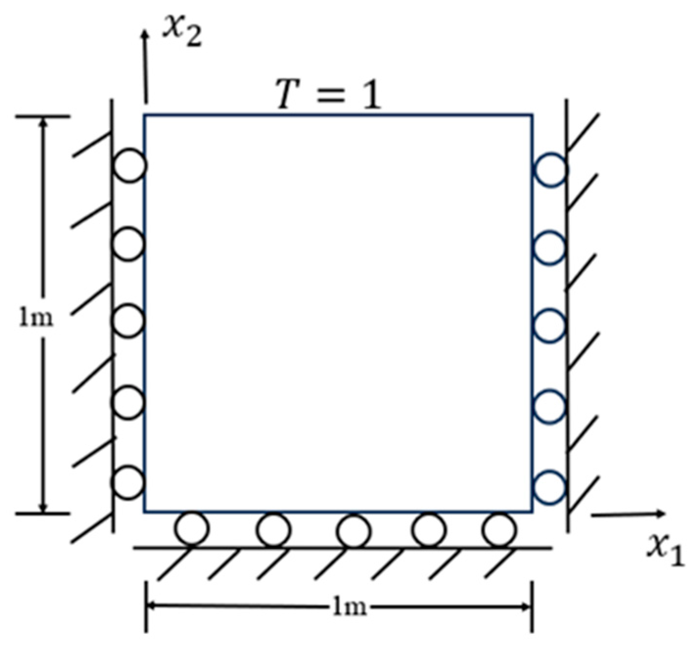
Consider a rectangular square plate under plane strain, as shown in Figure 1, where the top edge is subjected to a sudden thermal load, the other three edges are adiabatic, the left and right edges are constrained by displacement in the $x_1$ direction, and the bottom edge is constrained by displacement in the $x_2$ direction. The material parameters are: elastic modulus $E=\exp \left(x_2/10\right)\mathrm{P}\mathrm{a}$, Poisson’s ratio $v=0.3$, thermal conductivity $k=\exp \left(x_2/10\right)\mathrm{W}/(\mathrm{m}·°\mathrm{C})$, density $\rho =1 \mathrm{k}\mathrm{g}/{\mathrm{m}}^3$, specific heat capacity $C_p=1 \mathrm{J}/(\mathrm{k}\mathrm{g}·°\mathrm{C})$, and thermal expansion coefficient $\alpha =0.02/℃$. The distance from the field point to the source point is R = 0.045. The initial temperature, initial displacement, and velocity of the square plate are zero.

When the inertial and coupling terms are not considered, this problem is a quasi-static thermoelastic mechanics problem. In order to check the effect of the number of internal nodes on the results, the problem solution domain is discretized into 40 linear cells with 81 and 16 nodes arranged internally as shown in Figure 2a,b, and the time step is taken to be $\Delta t=0.001$ s. The results of the displacement and temperature fields obtained from the first 1.2 s are calculated using the RIBEM as a database for numerical simulation and from the displacement and temperature fields obtained from the first 1.2 s. The field variables at the moments of t = 0.1 s, 0.2 s, 0.3 s, … 1.2 s (total 12) are selected as the 12 snapshot vectors, which constitute the snapshot matrix $\mathit{A}$. 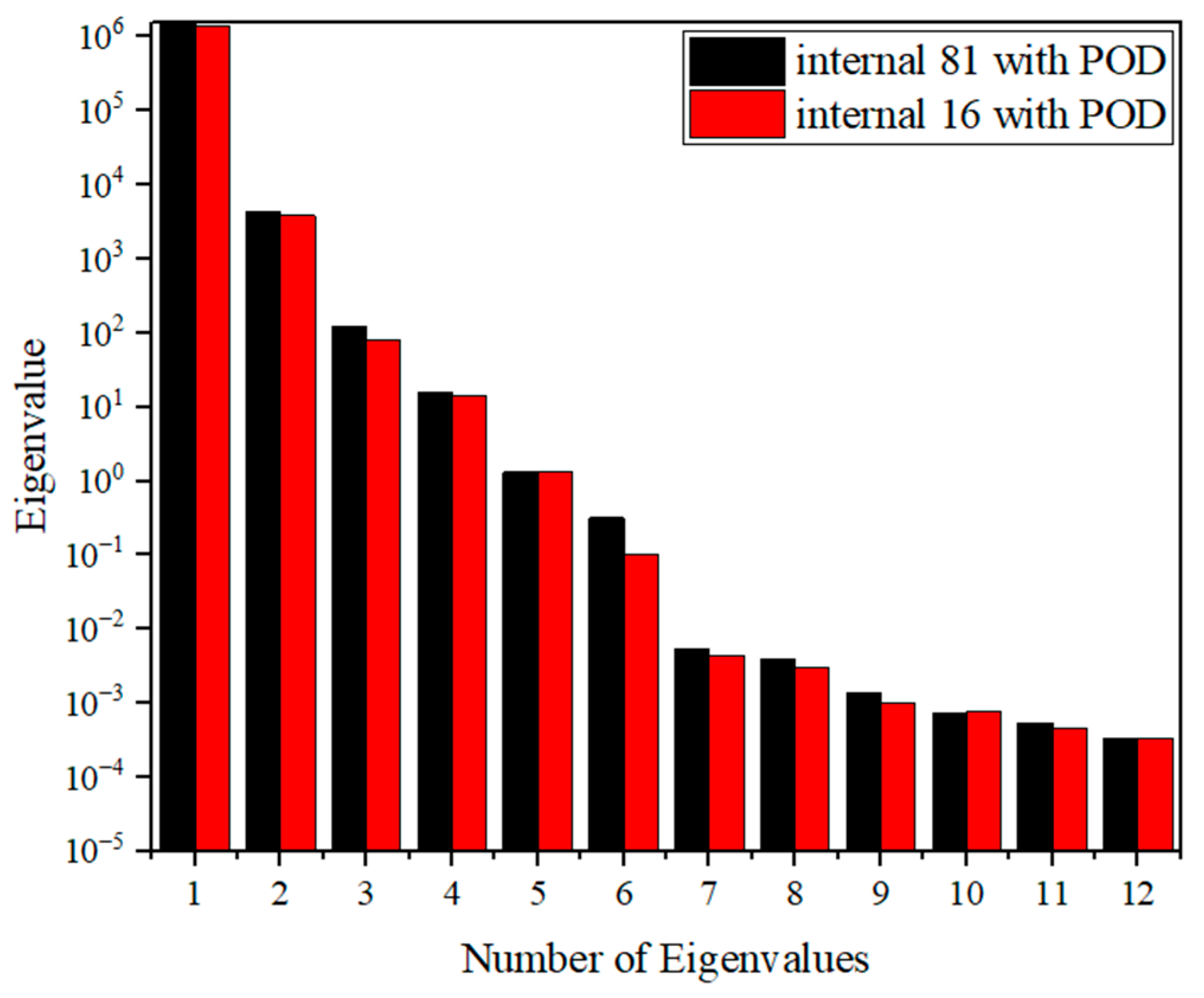The effect of adopting boundary element models with different numbers of internal nodes on the calculation results is compared and analyzed. The eigenvalues of the correlation matrix are listed as shown in Figure 3. The eigenvalues corresponding to the first five POD modes and their share of the system energy are given in

Table 1. Eigenvalues contribution of the first five orders in the quasi-static case.

K	${\mathit{\lambda }}_{\mathit{k}}$ (Internal 81)	${\displaystyle \sum _{\mathit{j}=1}^{\mathit{k}}}{\mathit{\lambda }}_{\mathit{j}}/{\displaystyle \sum _{\mathit{i}}}{\mathit{\lambda }}_{\mathit{i}}\times 100\mathit{\%}$	${\mathit{\lambda }}_{\mathit{k}}$ (Internal 16)	${\displaystyle \sum _{\mathit{j}=1}^{\mathit{k}}}{\mathit{\lambda }}_{\mathit{j}}/{\displaystyle \sum _{\mathit{i}}}{\mathit{\lambda }}_{\mathit{i}}\times 100\mathit{\%}$
1	1.5052 × 106	99.7009322	1.4061 × 106	99.7226477
2	4.3752 × 103	99.9907337	3.8168 × 103	99.9933306
3	122.6358	99.9988566	78.4818	99.9988963
4	15.6371	99.9998923	14.2869	99.9998988
5	1.2973	99.9999783	1.3121	99.9999918

. When $I\ge 99.9999\mathrm{\%}$ is satisfied, at this point K can be taken as 4 to establish a quasi-static reduced-order model of the rectangular square plate for both boundary element models, with internal node numbers 81 and 16, respectively. K can all be taken as 4 to establish a quasi-static ROM for a rectangular square plate.

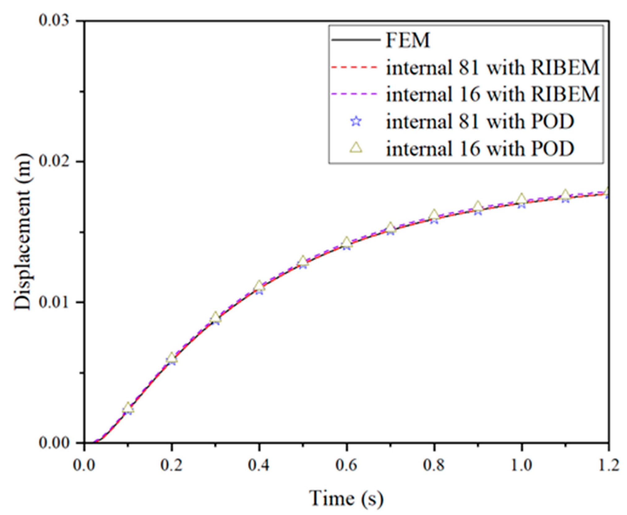
The results of temperature, displacement, and stress at point A (0, 0.5) obtained by the reduced-order model are shown in Figure 4, Figure 5 and Figure 6. They are compared with the RIBEM results and the finite element results obtained with the simulation software COMSOL Multiphysics 6.1 to verify the accuracy of the reduced-order model solution. Obviously, the solution of the reduced-order model and the solution of the RIBEM are very consistent with the comparison with the finite element results, so the number of internal nodes can be appropriately reduced under the premise of guaranteeing the accuracy of the solution, which in turn speeds up the large amount of time spent on the preparation of the transient matrix in the preliminary stage. As shown in

Table 2. Computation time for FOM and ROM in the quasi-static case.

Method	Degree of Freedom	Computation Time/s
FOM (internal 81)	363	29.9173
FOM (internal 16)	168	27.2681
ROM (internal 81)	4	1.3185
ROM (internal 16)	4	1.0748

, the degree of freedom is reduced from 363 to 4 when the internal nodes are taken as 81, and the solution degree of freedom is reduced from 168 to 4 when the internal nodes are taken as 16, which is a significant reduction in the solution degree of freedom. Moreover, compared with FOM, the reduced-order model effectively improves the computational efficiency.

4.2. Unilateral Fixed Plate under Time-Varying Loads

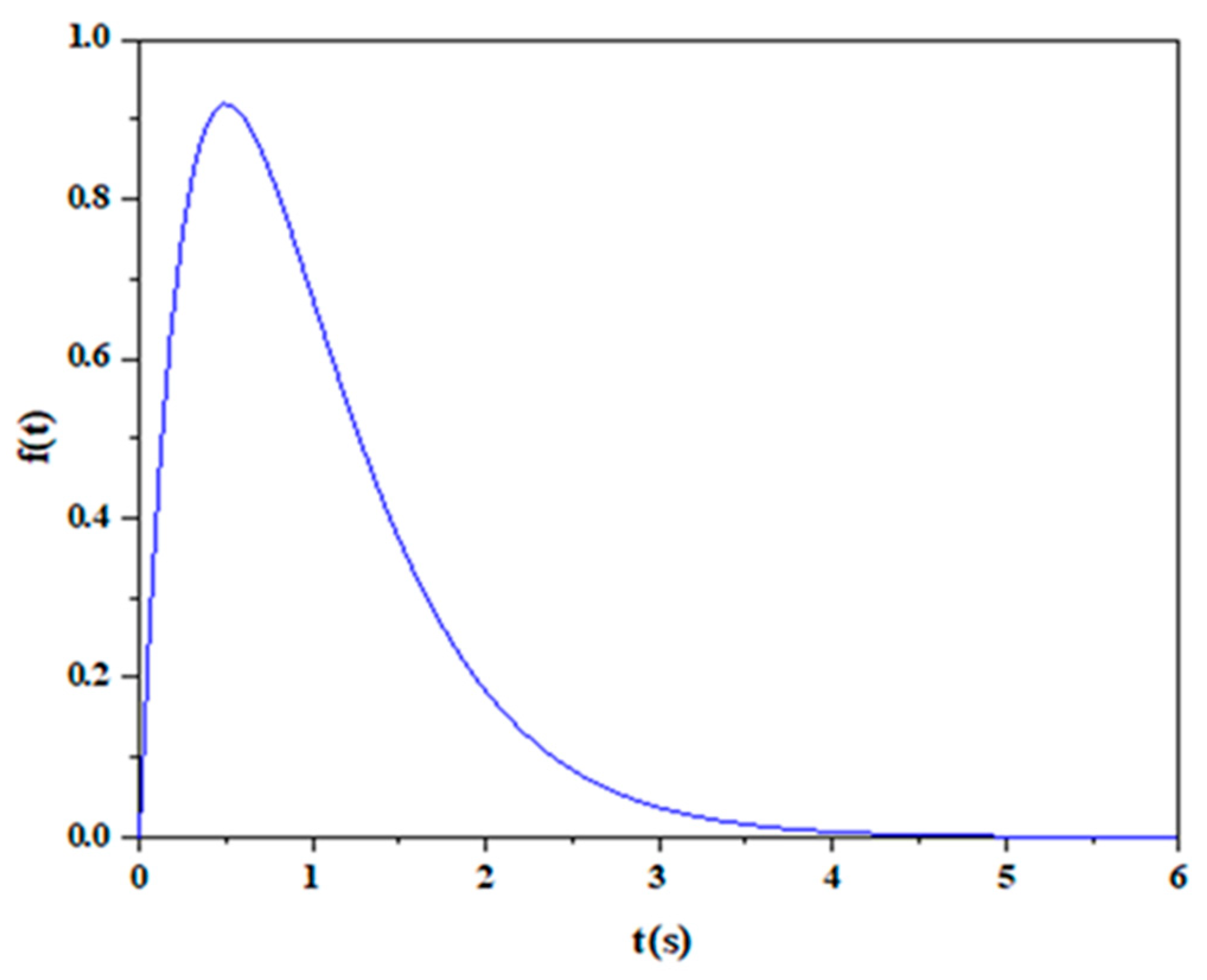
Consider a thermoelastic dynamics problem with fully coupled thermomechanical loads in a plane-strain state such as the square plate shown in Figure 7a, with a side length of 10 × 10 m, the right end fixed and adiabatic, the top and bottom sides free and adiabatic, and a uniformly distributed thermal load or mechanical pressure load $f\left(t\right)=5t\exp \left(-2t\right)$ applied to the left as shown in Figure 8. The square plate is initially stationary and the initial temperature is zero. The material parameters are: elastic modulus $E=\mathrm{e}\mathrm{x}\mathrm{p}\left(x_1∕l\right)\mathrm{P}\mathrm{a}$, Poisson’s ratio $v=0.3$, thermal conductivity $k=\mathrm{e}\mathrm{x}\mathrm{p}\left(x_1∕l\right)\mathrm{W}/(\mathrm{m}·°\mathrm{C})$, density $\rho =1 \mathrm{k}\mathrm{g}/{\mathrm{m}}^3$, specific heat capacity $C_p=1 \mathrm{J}/(\mathrm{k}\mathrm{g}·°\mathrm{C})$, and thermal expansion coefficient $\alpha =0.02/℃$. The calculation model is shown in Figure 7. The computational model of the square plate is shown in Figure 7b, where the boundary is discretized into 80 linear cells with an internal arrangement of 361 nodes, and the time step is taken as $\Delta t=1\times {10}^{-4}$ s. Furthermore, utilizing the commercial software COMSOL, the finite element mesh distribution is as shown in Figure 9.

In this example, the thermal coupling step-down analysis is carried out by introducing the coupling coefficient $\eta$ [49] as a measure of the level of thermoelastic coupling, and the thermal coupling step-down analysis is carried out for the case of the square plate coupled and uncoupled under thermal, mechanical, and combined thermomechanical loads, respectively. The coupling case is not considered when $\eta =0$. The corresponding coupling coefficient in this example is $\eta =0.1$.

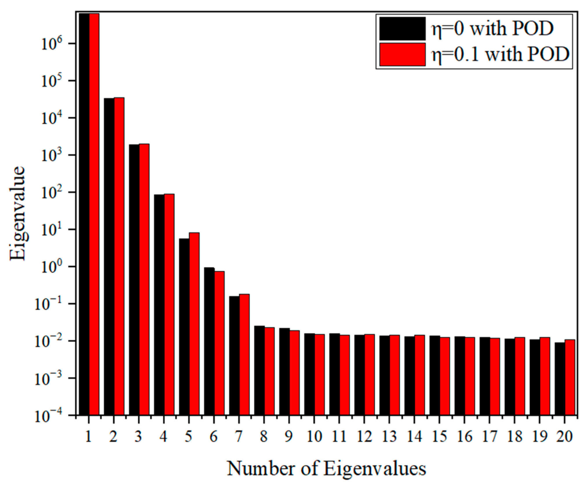
(1) Thermal shock loading alone: In this algorithm, the temperature on the left side of the square plate is shown in Figure 8 as a function of time, and the surface force on that side is zero. Snapshots are extracted at 0.3 s intervals, and the snapshots are subsequently subjected to an intrinsic orthogonal decomposition. The eigenvalue distributions for the coupled and uncoupled cases are presented separately, as shown in Figure 10.

Table 3. Eigenvalues contribution of the first five orders under thermal shock loading.

K	${\mathit{\lambda }}_{\mathit{k}}$$(\mathit{\eta }=0$)	${\displaystyle \sum _{\mathit{j}=1}^{\mathit{k}}}{\mathit{\lambda }}_{\mathit{j}}/{\displaystyle \sum _{\mathit{i}}}{\mathit{\lambda }}_{\mathit{i}}\times 100\mathit{\%}$	${\mathit{\lambda }}_{\mathit{k}}$$(\mathit{\eta }=0.1$)	${\displaystyle \sum _{\mathit{j}=1}^{\mathit{k}}}{\mathit{\lambda }}_{\mathit{j}}/{\displaystyle \sum _{\mathit{i}}}{\mathit{\lambda }}_{\mathit{i}}\times 100\mathit{\%}$
1	6.2647 × 106	99.4263703	6.2538 × 106	99.4009234
2	3.4147 × 104	99.9687344	3.5623 × 104	99.9671292
3	1.8751 × 103	99.9984922	1.9693 × 103	99.9984253
4	87.7142	99.9998908	89.5846	99.9998492
5	5.5841	99.9999794	8.3517	99.9999819

shows the eigenvalues corresponding to the first five orders of the POD modes and their share of the system energy, and it is easy to see that the eigenvalues of the coupled and uncoupled cases are not much different. Therefore, when $I\ge 99.9999\%$, the POD optimal base of 4 is chosen for the analysis. Numerical results of the distribution of temperature, displacement, and axial stress along the $x_1$ axis at time t = 3 s and t = 6 s are given in Figure 11a–f. The results show that there is good agreement between the down-order model and the full-order model comparison under thermal shock loading. As shown in

Table 4. Computation time for FOM and ROM under thermal shock loading.

Method	Degree of Freedom	Computation Time/s
FOM ($\eta =0$)	1323	182.6483
FOM ($\eta =0.1$)	1323	191.3618
ROM ($\eta =0$)	4	3.3185
ROM ($\eta =0$.1)	4	3.0748

, the establishment of the descending-order model effectively reduces the computational degrees of freedom of the RIBEM for solving the coupled thermoelastic problem under thermal shock loading and saves computational time.

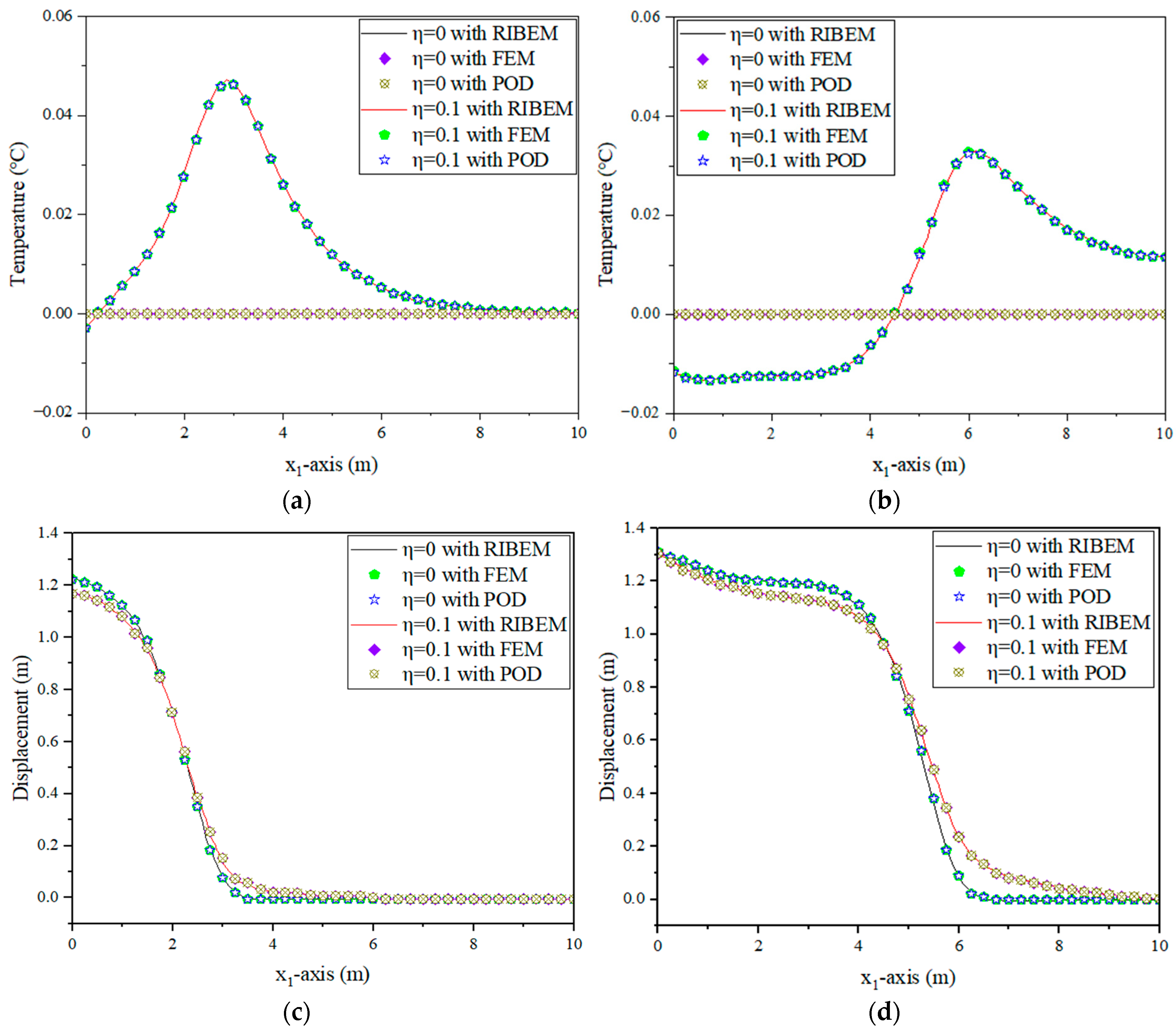
(2) Mechanical impact load alone: With other boundary conditions being the same, a mechanical impact load as shown in Figure 8 is applied to the left side of the square plate and adiabatic heat is applied on that side. Snapshots are extracted at 0.3 s intervals, as shown in Figure 12, which shows the distribution of eigenvalues under mechanical shock loading.

Table 5. Eigenvalues contribution of the first five orders under pressure shock loading.

K	${\mathit{\lambda }}_{\mathit{k}}$$(\mathit{\eta }=0$)	${\displaystyle \sum _{\mathit{j}=1}^{\mathit{k}}}{\mathit{\lambda }}_{\mathit{j}}/{\displaystyle \sum _{\mathit{i}}}{\mathit{\lambda }}_{\mathit{i}}\times 100\mathit{\%}$	${\mathit{\lambda }}_{\mathit{k}}$$(\mathit{\eta }=0.1$)	${\displaystyle \sum _{\mathit{j}=1}^{\mathit{k}}}{\mathit{\lambda }}_{\mathit{j}}/{\displaystyle \sum _{\mathit{i}}}{\mathit{\lambda }}_{\mathit{i}}\times 100\mathit{\%}$
1	5.2647 × 106	99.3538916	5.2453 × 106	99.3335292
2	3.2684 × 104	99.9706990	3.3695 × 104	99.9716432
3	1.4945 × 103	99.9989032	1.4348 × 103	99.9988156
4	52.6167	99.9998962	54.5392	99.9998484
5	4.3187	99.9999777	6.9318	99.9999797

shows the eigenvalues corresponding to the first five orders of the POD modes and their share of the system energy, and it is easy to see that there is not much difference between the eigenvalues of the coupled and uncoupled cases. Therefore, when $I\ge 99.9999\%$, K = 4 is chosen for the reduced-order analysis. 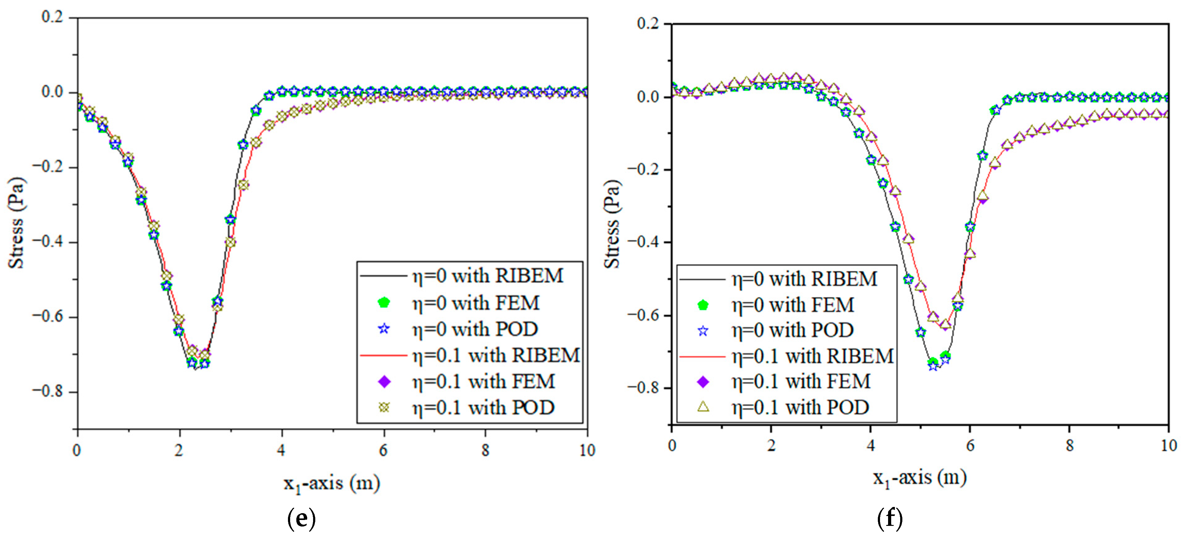The numerical results of the distributions of temperature, displacement, and axial stress along the $x_1$ axis when subjected to mechanical shock loading only for 3 s and 6 s are given in Figure 13a–f. Due to the effect of the coupling term, the values of the displacements and the stresses are smaller in the case where the coupling case is considered than in the case where the coupling is not considered. The results show that there is good agreement between the reduced-order model and the RIBEM and finite element results comparison. Similarly, the comparison of the computational efficiency between the full-order model and the reduced-order model is shown in

Table 6. Computation time for FOM and ROM under pressure shock loading.

Method	Degree of Freedom	Computation Time/s
FOM ($\eta =0$)	1323	187.3476
FOM ($\eta =0.1$)	1323	189.5924
ROM ($\eta =0$)	4	3.5974
ROM ($\eta =0$.1)	4	4.1908

, where the reduced-order modeling effectively saves computational time.

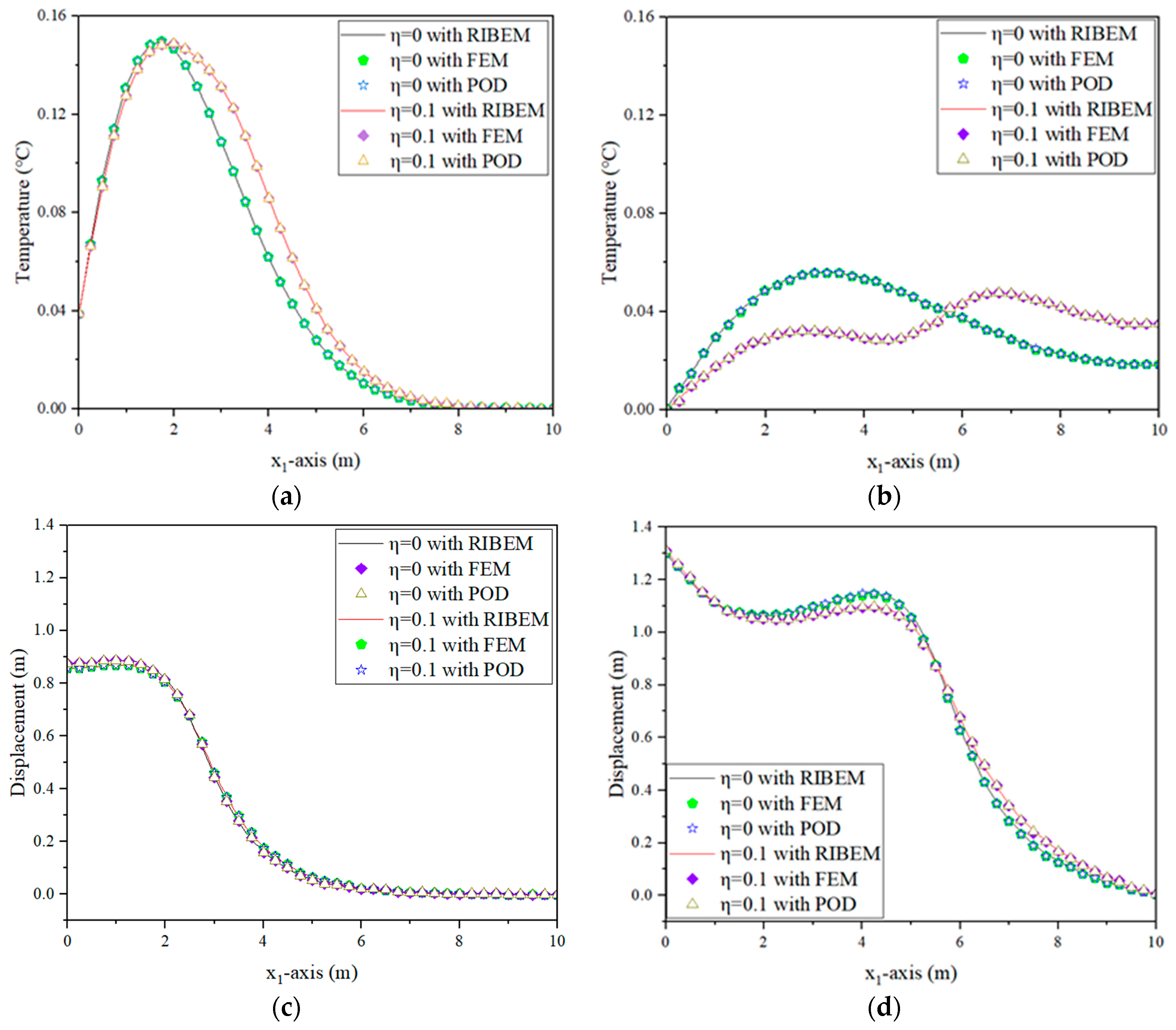
(3) Thermal and pressure shock in combination: In this case, both temperature loads and mechanical shock loads are applied to the left side of the square plate, as shown in Figure 8. The distributions of the eigenvalues under 20 combinations of thermomechanical shock loads are shown in Figure 14.

Table 7. Eigenvalues contribution of the first five orders under pressure shock loading.

K	${\mathit{\lambda }}_{\mathit{k}}$$(\mathit{\eta }=0$)	${\displaystyle \sum _{\mathit{j}=1}^{\mathit{k}}}{\mathit{\lambda }}_{\mathit{j}}/{\displaystyle \sum _{\mathit{i}}}{\mathit{\lambda }}_{\mathit{i}}\times 100\mathit{\%}$	${\mathit{\lambda }}_{\mathit{k}}$$(\mathit{\eta }=0.1$)	${\displaystyle \sum _{\mathit{j}=1}^{\mathit{k}}}{\mathit{\lambda }}_{\mathit{j}}/{\displaystyle \sum _{\mathit{i}}}{\mathit{\lambda }}_{\mathit{i}}\times 100\mathit{\%}$
1	7.4976 × 106	99.3883756	7.4169 × 106	99.3627968
2	4.3694 × 104	99.9675843	4.4928 × 104	99.9646975
3	2.3498 × 103	99.9987336	2.5364 × 103	99.9986773
4	87.3654	99.9998917	89.6492	99.9998783
5	6.6496	99.9999798	7.6149	99.9999804

shows the eigenvalues corresponding to the first five orders of POD modes and their share of the system energy. Therefore, when $I\ge 99.9999\mathrm{\%}$, K is taken as 4 for the reduced-order analysis. Figure 15a–f shows the numerical results for temperature, displacement, and stress, respectively.

Table 8. Computation time for FOM and ROM under thermal and pressure shock in combination.

Method	Degree of Freedom	Computation Time/s
FOM ($\eta =0$)	1323	213.7054
FOM ($\eta =0.1$)	1323	125.7136
ROM ($\eta =0$)	4	4.1873
ROM ($\eta =0$.1)	4	4.7531

shows the comparison of the computation time between the full-order model and the reduced-order model. The results show that the reduced-order model maintains a high computational accuracy while the computational efficiency is greatly improved.

4.3. FGM Thick Plate

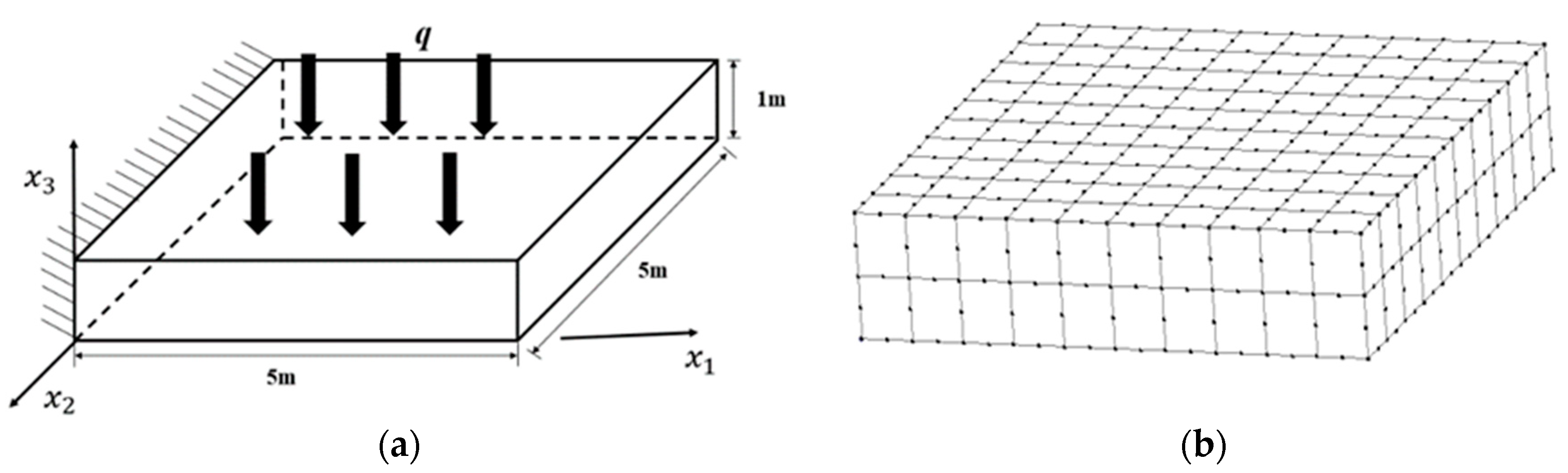
Consider a three-dimensional thick plate, shown in Figure 16a, where the upper surface of the plate is subjected to a uniformly distributed heat flow shock load $q=10 \mathrm{W}/{\mathrm{m}}^2$, with the left side being fixed and the other sides assumed to be adiabatic. The geometrical dimensions of the plate are 5 × 5 × 1 m. The material parameters are: elastic modulus $E=\mathrm{e}\mathrm{x}\mathrm{p}\left(x_1∕10\right)\mathrm{P}\mathrm{a}$, Poisson’s ratio $v=0.28$, thermal conductivity $k=\mathrm{e}\mathrm{x}\mathrm{p}\left(x_1∕10\right) \mathrm{W}/(\mathrm{m}·°\mathrm{C})$, density $\rho =1 \mathrm{k}\mathrm{g}/{\mathrm{m}}^3$, specific heat capacity $C_p=1 \mathrm{J}/(\mathrm{k}\mathrm{g}·°\mathrm{C})$, and thermal expansion coefficient $\alpha =0.02/℃$. Figure 16b shows the computational model of the boundary element method for a 3D thick plate, where the boundary is discretized into 280 quadratic units with 842 boundary nodes and 361 nodes arranged internally, and the time step is taken as $\Delta t=1\times {10}^{-6} \mathrm{s}$. The boundary is discretized into 280 quadratic units with 842 boundary nodes and 361 nodes arranged internally.

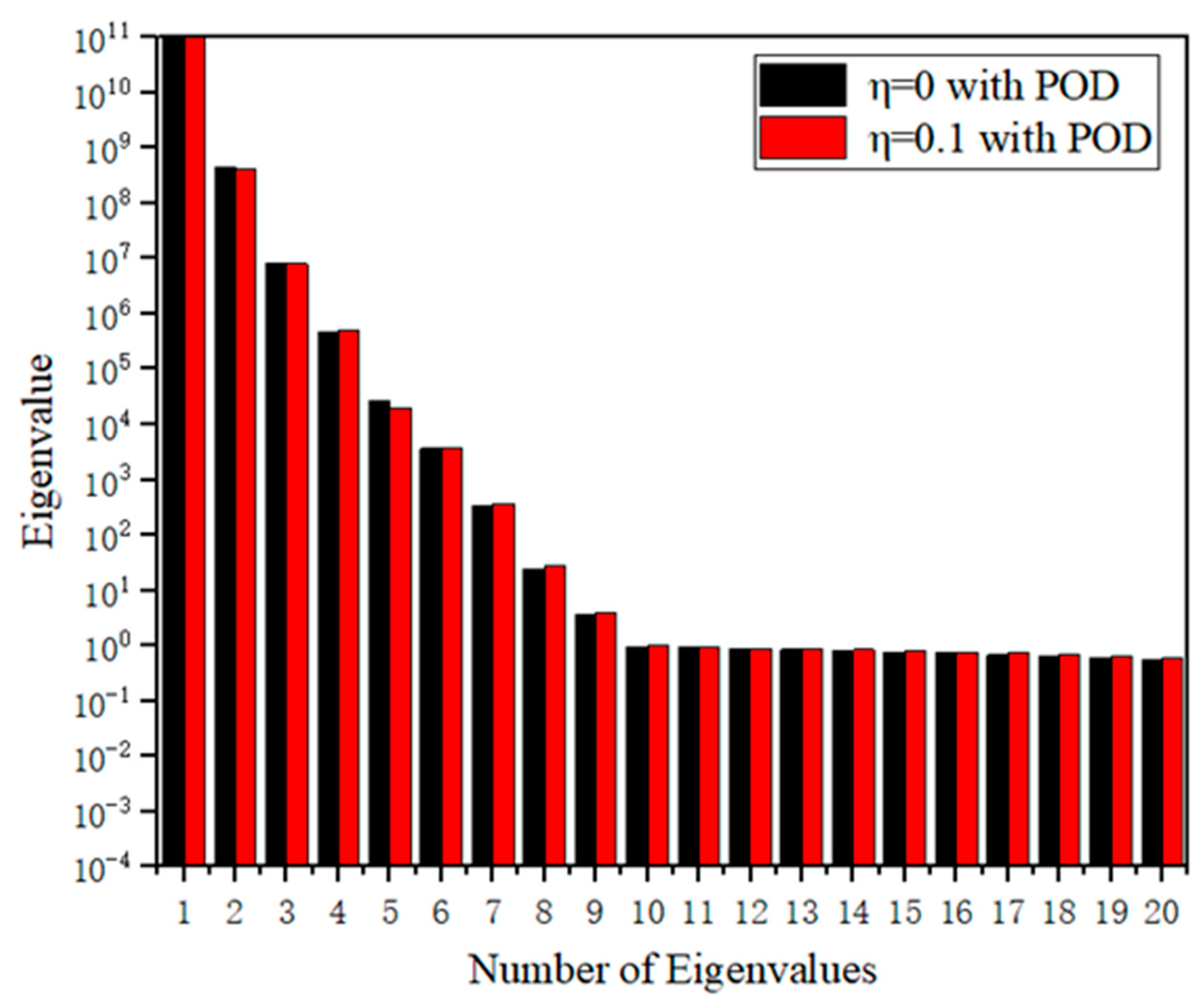
Assuming that the temperature of the thick plate at the initial moment is 0, its corresponding coupling parameter is about η = 0.1. After solving the 3D heat flow impact loading problem described above, the temperature and displacement field data are extracted at intervals of 0.002 s. The temperature and displacement field data are extracted at the same time. As shown in Figure 17 and

Table 9. Eigenvalues and their percentage of system energy for the FGM thick plate (the first six orders).

K	${\mathit{\lambda }}_{\mathit{k}}$ $(\mathit{\eta }=0$)	${\displaystyle \sum _{\mathit{j}=1}^{\mathit{k}}}{\mathit{\lambda }}_{\mathit{j}}/{\displaystyle \sum _{\mathit{i}}}{\mathit{\lambda }}_{\mathit{i}}\times 100\mathit{\%}$	${\mathit{\lambda }}_{\mathit{k}}$ $(\mathit{\eta }=0.1$)	${\displaystyle \sum _{\mathit{j}=1}^{\mathit{k}}}{\mathit{\lambda }}_{\mathit{j}}/{\displaystyle \sum _{\mathit{i}}}{\mathit{\lambda }}_{\mathit{i}}\times 100\mathit{\%}$
1	1.5374 × 1011	99.7117507	1.4206 × 1011	99.7025275
2	4.3548 × 108	99.9941927	4.1548 × 108	99.9941092
3	8.4535 × 106	99.9996754	7.8862 × 106	99.9996437
4	4.6948 × 105	99.9999799	4.8384 × 105	99.9999832
5	2.6824 × 104	99.9999973	1.9572 × 104	99.9999970
6	3.6535 × 103	99.9999997	3.8561 × 103	99.9999997

, as with the 1D and 2D simplified models, the higher order eigenvalues in the 3D model account for the largest energy. The eigenvalues corresponding to the first six POD modes and their share of the system energy are shown in Table 9. Therefore, when $I>99.99999\%$, K = 4 is chosen for the reduced-order analysis. Figure 18a shows the temperature at point M (5, 0, 0.5) as a function of time, and Figure 18b gives the results of the numerical analysis of the vertical displacement at point M. From Figure 18a,b, it is obvious that the 3D step-down model is still in good agreement with the FOM. On the other hand, as shown in

Table 10. Computation time of FOM and ROM of the FGM thick plate in coupled and uncoupled cases.

Method	Degree of Freedom	Computation Time/s
FOM ($\eta =0$)	4812	613.6481
FOM ($\eta =0.1$)	4812	631.8459
ROM ($\eta =0$)	4	5.6982
ROM ($\eta =0$.1)	4	5.8413

, the introduction of the reduced-order model significantly reduces the degrees of freedom and improves the computational efficiency by more than 100 times. However, the acquisition of the snapshot matrix is time-consuming, so the research on POD still has great potential.

5. Conclusions

In this paper, the radial integral boundary element method is firstly adopted to analyze and solve the thermal coupling problem, and the temperature and displacement fields obtained with the RIBEM are used to establish a database to construct a low-dimensional and orthogonal POD substrate, and then hundreds of thousands of degrees of freedom problems are projected into the low-dimensional space for analysis. The model can quickly solve the thermal coupling problem of functionally gradient materials.

(i)

The dependence of the computational results on the distribution of internal nodes is examined by using different numbers of internal nodes. The numerical results of the method in this paper are not too sensitive to the number of internal nodes, and a small number of nodes arranged internally can obtain satisfactory results. However, for nonuniform initial conditions, a suitable number of nodes must be arranged in the computational domain to ensure the accuracy of the calculation results.

(ii)

In order to analyze the thermal coupling without coupling and with coupling, this paper constructs two kinds of transient matrices without coupling and with coupling, obtains the two sets of optimal POD bases, and establishes the POD step-down model. The results of the POD step-down are in good consistency with the full-order model of the finite element and the boundary element.

(iii)

To construct the ROM for the thermal coupling problem of functionally gradient materials, the computational time is mainly consumed in the acquisition of snapshots of the FGMs using the RIBEM. Once the POD bases of the functionally gradient materials are obtained, the temperatures, displacements, and stresses under different dynamic loads can be solved quickly, and the time for solving the reduced-order model will be much shorter than that for the calculation of the FOM.

In summary, this study proposes a fast reduced-order algorithm based on the RIBEM and POD, effectively reducing the computational time cost for solving the thermal coupling problem of FGMs while ensuring a high level of accuracy. A potential avenue for future research could involve extending the applicability of thermal coupling analysis by integrating the hyper-reduction method [50,51,52] with the RIBEM to address nonlinear problems associated with temperature-dependent material parameters.

References

1. Delfosse, D.; Suresh, S.; Mortensen, A. Fundamentals of Functionally Graded Materials; IOM Communications Ltd.: London, UK, 1998; ISBN 1-86125-063-0. [Google Scholar]
2. Lee, W.Y.; Stinton, D.P.; Berndt, C.C.; Erdogan, F.; Lee, Y.D.; Mutasim, Z. Concept of functionally graded materials for advanced thermal barrier coating applications. J. Am. Ceram. Soc. 1996, 79, 3003–3012. [Google Scholar] [CrossRef]
3. Watari, F.; Yokoyama, A.; Omori, M.; Hirai, T.; Kondo, H.; Uo, M.; Kawasaki, T. Biocompatibility of materials and development to functionally graded implant for bio-medical application. Compos. Sci. Technol. 2004, 64, 893–908. [Google Scholar] [CrossRef]
4. Pompe, W.; Worch, H.; Epple, M.; Friess, W.; Gelinsky, M.; Greil, P.; Hempel, U.; Scharnweber, D.; Schulte, K. Functionally graded materials for biomedical applications. Mater. Sci. Eng. A 2003, 362, 40–60. [Google Scholar] [CrossRef]
5. Schulz, U.; Peters, M.; Bach, F.-W.; Tegeder, G. Graded coatings for thermal, wear and corrosion barriers. Mater. Sci. Eng. A 2003, 362, 61–80. [Google Scholar] [CrossRef]
6. Lengauer, W.; Dreyer, K. Functionally graded hardmetals. J. Alloys Compd. 2002, 338, 194–212. [Google Scholar] [CrossRef]
7. Hart, N.; Brandon, N.; Day, M.; Lapena-Rey, N. Functionally graded composite cathodes for solid oxide fuel cells. J. Power Sources 2002, 106, 42–50. [Google Scholar] [CrossRef]
8. Williamson, R.; Rabin, B.; Drake, J. Finite element analysis of thermal residual stresses at graded ceramic-metal interfaces. Part I. Model description and geometrical effects. J. Appl. Phys. 1993, 74, 1310–1320. [Google Scholar] [CrossRef]
9. Drake, J.; Williamson, R.; Rabin, B. Finite element analysis of thermal residual stresses at graded ceramic-metal interfaces. Part II. Interface optimization for residual stress reduction. J. Appl. Phys. 1993, 74, 1321–1326. [Google Scholar] [CrossRef]
10. Hosseini, S.M.; Akhlaghi, M. Analytical solution in transient thermo-elasticity of functionally graded thick hollow cylinders (Pseudo-dynamic analysis). Math. Methods Appl. Sci. 2009, 32, 2019–2034. [Google Scholar] [CrossRef]
11. Zheng, B.J.; Gao, X.W.; Yang, K.; Zhang, C.Z. A novel meshless local Petrov–Galerkin method for dynamic coupled thermoelasticity analysis under thermal and mechanical shock loading. Eng. Anal. Bound. Elem. 2015, 60, 154–161. [Google Scholar] [CrossRef]
12. Sutradhar, A.; Paulino, G.H. The simple boundary element method for transient heat conduction in functionally graded materials. Comput. Methods Appl. Mech. Eng. 2004, 193, 4511–4539. [Google Scholar] [CrossRef]
13. Dominguez, J. Boundary element approch for dynamic poroelastic problems. Int. J. Numer. Methods Eng. 1992, 35, 307–324. [Google Scholar] [CrossRef]
14. Dargush, G.; Banerjee, P. A new boundary element method for three-dimensional coupled problems of consolidation and thermoelasticity. Eng. Anal. Bound. Elem. 1991, 16, 297–303. [Google Scholar] [CrossRef]
15. Gao, X.W. The radial integration method for evaluation of domain integrals with boundary-only discretization. Eng. Anal. Bound. Elem. 2002, 26, 905–916. [Google Scholar] [CrossRef]
16. Gao, X.W.; Zheng, B.J.; Yang, K.; Zhang, C. Radial integration BEM for dynamic coupled thermoelastic analysis under thermal shock loading. Comput. Struct. 2015, 158, 140–147. [Google Scholar] [CrossRef]
17. Gao, X.W. A boundary element method without internal cells for two-dimensional and three-dimensional elastoplastic problems. J. Appl. Mech. 2002, 69, 154–160. [Google Scholar] [CrossRef]
18. Yang, K.; Wang, J.; Du, J.M.; Peng, H.F.; Gao, X.W. Radial integration boundary element method for nonlinear heat conduction problems with temperature-dependent conductivity. Int. J. Heat Mass Transf. 2017, 104, 1145–1151. [Google Scholar] [CrossRef]
19. Yang, K.; Feng, W.Z.; Peng, H.F.; Lv, J. A new analytical approach of functionally graded material structures for thermal stress BEM analysis. Int. Commun. Heat Mass Transf. 2015, 62, 26–32. [Google Scholar] [CrossRef]
20. Peng, H.F.; Yang, K.; Cui, M.; Gao, X.W. Radial integration boundary element method for solving two-dimensional unsteady convection–diffusion problem. Eng. Anal. Bound. Elem. 2019, 102, 39–50. [Google Scholar] [CrossRef]
21. Yu, B.; Yao, W.A.; Gao, X.W.; Gao, Q. A combined approach of RIBEM and precise time integration algorithm for solving transient heat conduction problems. Numer. Heat Transf. Part B Fundam. 2014, 65, 155–173. [Google Scholar] [CrossRef]
22. Smith, T.R.; Moehlis, J.; Holmes, P. Low-dimensional modelling of turbulence using the proper orthogonal decomposition: A tutorial. Nonlinear Dyn. 2005, 41, 275–307. [Google Scholar] [CrossRef]
23. Kunisch, K.; Volkwein, S. Galerkin proper orthogonal decomposition methods for a general equation in fluid dynamics. SIAM J. Numer. Anal. 2002, 40, 492–515. [Google Scholar] [CrossRef]
24. LeGresley, P.; Alonso, J. Investigation of non-linear projection for pod based reduced order models for aerodynamics. In Proceedings of the 39th Aerospace Sciences Meeting and Exhibit, Reno, NV, USA, 8–11 January 2001; p. 926. [Google Scholar]
25. Bui-Thanh, T.; Damodaran, M.; Willcox, K. Proper orthogonal decomposition extensions for parametric applications in compressible aerodynamics. In Proceedings of the 21st AIAA Applied Aerodynamics Conference, Orlando, FL, USA, 23–26 June 2003; p. 4213. [Google Scholar]
26. Gao, X.W.; Hu, J.X.; Huang, S.Z. A proper orthogonal decomposition analysis method for multimedia heat conduction problems. J. Heat Transf. 2016, 138, 071301. [Google Scholar] [CrossRef]
27. Liang, Y.; Gao, X.W.; Xu, B.B.; Zhu, Q.H.; Wu, Z.Y. A new alternating iteration strategy based on the proper orthogonal decomposition for solving large-scaled transient nonlinear heat conduction problems. J. Comput. Sci. 2020, 45, 101206. [Google Scholar] [CrossRef]
28. Fic, A.; Białecki, R.A.; Kassab, A.J. Solving transient nonlinear heat conduction problems by proper orthogonal decomposition and the finite-element method. Numer. Heat Transf. Part B Fundam. 2005, 48, 103–124. [Google Scholar] [CrossRef]
29. Jiang, G.H.; Liu, H.Y.; Yang, K.; Gao, X.W. A fast reduced-order model for radial integral boundary element method based on proper orthogonal decomposition in nonlinear transient heat conduction problems. Comput. Methods Appl. Mech. Eng. 2020, 368, 113190. [Google Scholar] [CrossRef]
30. Tang, Z.B.; Hu, J.X.; Li, Z.J. A reduced-order modeling for thermo-mechanical coupling analyses by using radial integration boundary element method. Eng. Anal. Bound. Elem. 2023, 156, 211–222. [Google Scholar] [CrossRef]
31. Xie, G.Z.; Zhong, Y.D.; Zhou, F.L.; Du, W.L.; Li, H.; Zhang, D.H. Singularity cancellation method for time-domain boundary element formulation of elastodynamics: A direct approach. Appl. Math. Model. 2020, 80, 647–667. [Google Scholar] [CrossRef]
32. Lei, W.D.; Li, H.J.; Qin, X.F.; Chen, R.; Ji, D.F. Dynamics-based analytical solutions to singular integrals for elastodynamics by time domain boundary element method. Appl. Math. Model. 2018, 56, 612–625. [Google Scholar] [CrossRef]
33. Gao, X.W. An effective method for numerical evaluation of general 2D and 3D high order singular boundary integrals. Comput. Methods Appl. Mech. Eng. 2010, 199, 2856–2864. [Google Scholar] [CrossRef]
34. Balas, J.; Sladek, J.; Sladek, V. Stress Analysis by Boundary Element Methods; Elsevier: Amsterdam, The Netherlands, 2013. [Google Scholar]
35. Gao, X.W.; Zhang, C.; Guo, L. Boundary-only element Solutions of 2D and 3D nonlinear and nonhomogeneous elastic problems. Eng. Anal. Bound. Elem. 2007, 31, 974–982. [Google Scholar] [CrossRef]
36. Yang, K.; Peng, H.F.; Wang, J.; Xing, C.H.; Gao, X.W. Radial integration BEM for solving transient nonlinear heat conduction with temperature-dependent conductivity. Int. J. Heat Mass Transf. 2017, 108, 1551–1559. [Google Scholar] [CrossRef]
37. Ji, D.F.; Lei, W.D.; Li, H.J. Corner treatment by assigning dual tractions to every node for elastodynamics in TD-BEM. Appl. Math. Comput. 2016, 284, 125–135. [Google Scholar] [CrossRef]
38. Partridge, P.W.; Brebbia, C.A. Dual Reciprocity Boundary Element Method; Springer Science & Business Media: Cham, Switzerland, 2012. [Google Scholar]
39. Partridge, P.W.; Brebbia, C. Computer implementation of the BEM dual reciprocity method for the solution of general field equations. Commun. Appl. Numer. Methods 1990, 6, 83–92. [Google Scholar] [CrossRef]
40. Nowak, A.J.; Brebbia, C.A. The multiple-reciprocity method. A new approach for transforming BEM domain integrals to the boundary. Eng. Anal. Bound. Elem. 1989, 6, 164–167. [Google Scholar] [CrossRef]
41. Hematiyan, M.R.; Mohammadi, M.; Marin, L.; Khosravifard, A. Boundary element analysis of uncoupled transient thermo-elastic problems with time-and space-dependent heat sources. Appl. Math. Comput. 2011, 218, 1862–1882. [Google Scholar] [CrossRef]
42. Hematiyan, M.R.; Khosravifard, A.; Bui, T. Efficient evaluation of weakly/strongly singular domain integrals in the BEM using a singular nodal integration method. Eng. Anal. Bound. Elem. 2013, 37, 691–698. [Google Scholar] [CrossRef]
43. Ochiai, Y. Meshless thermo-elastoplastic analysis by triple-reciprocity boundary element method. Int. J. Numer. Methods Eng. 2010, 81, 1609–1634. [Google Scholar] [CrossRef]
44. Paulino, G.H.; Sutradhar, A.; Gruy, L. Boundary element methods for functionally graded materials. WIT Trans. Model. Simul. 2003, 34, 137–146. [Google Scholar]
45. Cui, M.; Peng, H.F.; Xu, B.B.; Gao, X.W.; Zhang, Y.W. A new radial integration polygonal boundary element method for solving heat conduction problems. Int. J. Heat Mass Transf. 2018, 123, 251–260. [Google Scholar] [CrossRef]
46. Houbolt, J.C. A recurrence matrix solution for the dynamic response of elastic aircraft. J. Aeronaut. Sci. 1950, 17, 540–550. [Google Scholar] [CrossRef]
47. Sirovich, L. Turbulence and the dynamics of coherent structures. I. Coherent structures. Q. Appl. Math. 1987, 45, 561–571. [Google Scholar] [CrossRef]
48. Chatterjee, A. An introduction to the proper orthogonal decomposition. Curr. Sci. 2000, 78, 808–817. [Google Scholar]
49. Cannarozzi, A.A.; Ubertini, F. A mixed variational method for linear coupled thermoelastic analysis. Int. J. Solids Struct. 2001, 38, 717–739. [Google Scholar] [CrossRef]
50. Ryckelynck, D. Hyper-reduction of mechanical models involving internal variables. Int. J. Numer. Methods Eng. 2009, 77, 75–89. [Google Scholar] [CrossRef]
51. Farhat, C.; Chapman, T.; Avery, P. Structure-preserving, stability, and accuracy properties of the energy-conserving sampling and weighting method for the hyper reduction of nonlinear finite element dynamic models. Int. J. Numer. Methods Eng. 2015, 102, 1077–1110. [Google Scholar] [CrossRef]
52. Kaneko, S.; Wei, H.; He, Q.; Chen, J.S.; Yoshimura, S. A hyper-reduction computational method for accelerated modeling of thermal cycling-induced plastic deformations. J. Mech. Phys. Solids 2021, 151, 104385. [Google Scholar] [CrossRef]
Figure 1. Suddenly heated rectangular plate.
Mathematics 11 03870 g001
Figure 2. Boundary element method computational modelling of square plates: (a) 81 internal nodes; (b) 16 internal nodes.
Mathematics 11 03870 g002
Figure 3. Distribution of eigenvalues for rectangular plate.
Mathematics 11 03870 g003
Figure 4. Change in temperature at point A with time.
Mathematics 11 03870 g004
Figure 5. Change in displacement u 2 of point A with time.
Mathematics 11 03870 g005
Figure 6. Variation in axial stress σ 11 at point A with time.
Mathematics 11 03870 g006
Figure 7. Rectangular square plates subjected to impact loads: (a) Geometric modelling; (b) Boundary element method computational model.
Mathematics 11 03870 g007
Figure 8. Pattern of the impulse load.
Mathematics 11 03870 g008
Figure 9. The finite element meshes of the plate.
Mathematics 11 03870 g009
Figure 10. Distribution of the eigenvalues of rectangular plates under thermal shock loading.
Mathematics 11 03870 g010
Figure 11. Under thermal loading: (a) Distribution of temperature along x 1 axis at t = 3 s; (b) Distribution of temperature along x 1 axis at t = 6 s; (c) Distribution of axial displacement along the x 1 axis at t = 3 s; (d) Distribution of axial displacement along the x 1 axis at t = 6 s; (e) Distribution of axial stress along the x 1 axis at t = 3 s; (f) Distribution of axial stress along the x 1 axis at t = 6 s.
Mathematics 11 03870 g011aMathematics 11 03870 g011b
Figure 12. Distribution of eigenvalues of rectangular plates under mechanical shock loading.
Mathematics 11 03870 g012
Figure 13. Under mechanical loading: (a) Distribution of temperature along x 1 axis at t = 3 s; (b) Distribution of temperature along x 1 axis at t = 6 s; (c) Distribution of axial displacement along the x 1 axis at t = 3 s; (d) Distribution of axial displacement along the x 1 axis at t = 6 s; (e) Distribution of axial stress along the x 1 axis at t = 3 s; (f) Distribution of axial stress along the x 1 axis at t = 6 s.
Mathematics 11 03870 g013aMathematics 11 03870 g013b
Figure 14. Distribution of eigenvalues of rectangular plates under combined loads.
Mathematics 11 03870 g014
Figure 15. Thermal and pressure shock in combination: (a) Distribution of temperature along x 1 axis at t = 3 s; (b) Distribution of temperature along x 1 axis at t = 6 s; (c) Distribution of axial displacement along the x 1 axis at t = 3 s; (d) Distribution of axial displacement along the x 1 axis at t = 6 s; (e) Distribution of axial stress along the x 1 axis at t = 3 s; (f) Distribution of axial stress along the x 1 axis at t = 6 s.
Mathematics 11 03870 g015aMathematics 11 03870 g015b
Figure 16. FGM thick plates subjected to thermal shock loads: (a) Geometric modelling; (b) Boundary element method computational model.
Mathematics 11 03870 g016
Figure 17. Distribution of eigenvalues for 3D thick plates.
Mathematics 11 03870 g017
Figure 18. (a) The temperature variation over time at point M on the thick plate; (b) The vertical displacement u 3 at point M on the thick plate as a function of time.
Mathematics 11 03870 g018