Fast Generalized Sliding Sinusoidal Transforms

Abstract

Discrete cosine and sine transforms closely approximate the Karhunen–Loeve transform for first-order Markov stationary signals with high and low correlation coefficients, respectively. Discrete sinusoidal transforms can be used in data compression, digital filtering, spectral analysis and pattern recognition. Short-time transforms based on discrete sinusoidal transforms are suitable for the adaptive processing and time–frequency analysis of quasi-stationary data. The generalized sliding discrete transform is a type of short-time transform, that is, a fixed-length windowed transform that slides over a signal with an arbitrary integer step. In this paper, eight fast algorithms for calculating various sliding sinusoidal transforms based on a generalized solution of a second-order linear nonhomogeneous difference equation and pruned discrete sine transforms are proposed. The performances of the algorithms in terms of computational complexity and execution time were compared with those of recursive sliding and fast discrete sinusoidal algorithms. The low complexity of the proposed algorithms resulted in significant time savings.

1. Introduction

Discrete cosine transform (DCT) and discrete sine transform (DST) are two of the most common unitary transforms in signal processing due to their close approximation to the Karhunen–Loeve transform (KLT) [1]. For signals with a correlation coefficient close to one, DCT provides a better approximation of KLT than DST, whereas DST is closer to KLT when the correlation coefficient is less than 0.5. Because KLT consists of eigenvectors of the covariance matrix of data, there is no single unique transform for all random processes, and there are no fast algorithms. In contrast, DCT and DST are data-independent, and many fast algorithms have been proposed.

Discrete sinusoidal transforms were originally introduced to process long-term stationary data [2]. They have found widespread application in various forms of signal processing such as data coding [3], adaptive digital filtering [4], image enhancement [5], interpolation [6,7]. Short-time signal processing [8] is an appropriate technique for time–frequency analyses and processing nonstationary data, such as ECG signal processing [9], spectral analysis and speech processing [10], adaptive linear filtering [5,11], radar emitter recognition [12], spectral analysis of biological signals [13], heart sound classification [14], and time–frequency analyses of supply voltage systems [15]. The hopping discrete transform [16,17,18] is a time series of equidistant windowed signal transforms. The generalized sliding discrete transform is a type of short-time transform in which a fixed-length windowed transform slides over a signal with arbitrary integer steps. In this case, the window signal is constantly updated with new samples, and the old samples are discarded. To obtain an acceptable spectral resolution, the window size must be such that the signal in the window can be considered approximately stationary. DCT and DST are important unitary transforms for the spectral analysis of time-varying signals. Because the computation of discrete sinusoidal transforms in a window sliding over a signal with one sample step is computationally expensive, fast algorithms have been proposed to compute eight types of transforms using recursive equations [19,20].

When the signal spectrum changes slowly, the window can move more than one sample at a time to speed up the spectral analysis. To quickly calculate the DCT in a window moving with small integer steps, a recursive sliding algorithm was proposed [21]. Recursive equations and fast algorithms have been proposed for calculating various types of generalized sliding DCTs [22] that can be turned as a trade-off between hardware consumption and performance.

Four types of DCT and four types of DST were classified [23]. This paper proposes eight fast algorithms for calculating sliding discrete sinusoidal transforms based on the derived recursive equations and fast-pruned DSTs. The contribution of this work is as follows:

• A generalized solution of a second-order linear nonhomogeneous difference equation is obtained using the unilateral z-transform.
• Based on the generalized solution, eight generalized sliding sinusoidal transforms are proposed.
• Fast algorithms have been proposed for computing generalized sliding sinusoidal transforms. The algorithms are based on the derived recursive equations and fast-pruned DSTs.
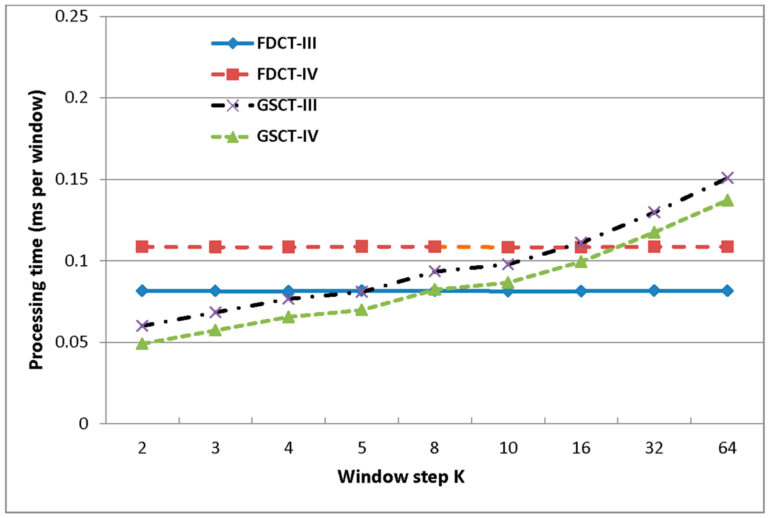
• The performance of the proposed algorithms in terms of computational complexity and execution time is compared with those of recursive sliding and fast sinusoidal algorithms.

The remainder of this paper is organized as follows. Section 2 introduces the notation and recalls the sliding discrete sinusoidal transforms. A generalized solution of a second-order linear nonhomogeneous difference equation and generalized sliding sinusoidal transforms are presented in Section 2. The design of the fast algorithms is presented in Section 3. In Section 4, the performances of the proposed, recursive sliding and well-known fast discrete sinusoidal algorithms with respect to computational complexity and execution time are presented and discussed. Section 5 summarizes our findings.

2. Generalized Sliding Discrete Sinusoidal Transforms

2.1. Sliding Discrete Sinusoidal Transforms

Let us recall the definition of sliding discrete sinusoidal transforms [20] using the following notation: ${\mathrm{sn}}_N\left(rs\right)\equiv \sin \left(\frac{\pi }{N}rs\right)$, $\mathrm{c}{\mathrm{s}}_N\left(rs\right)\equiv \cos \left(\frac{\pi }{N}rs\right)$, where N is the transform order, and $r,s\in R$.

The sliding cosine transforms (SCT) of types I, II, III, and IV can be defined as

$$\mathrm{SCT}-\mathrm{I}:y_s\left(k\right)={\displaystyle \sum _{n=-N_1}^{N_2}x\left(k+n\right){\mathrm{cs}}_N\left(s\left(n+N_1\right)\right)},$$

(1)

$$\mathrm{SCT}-\mathrm{II}: y_s\left(k\right)={\displaystyle \sum _{n=-N_1}^{N_2}x\left(k+n\right){\mathrm{cs}}_N\left(s\left(n+N_1+1/2\right)\right)},$$

(2)

$$\mathrm{SCT}-\mathrm{III}: y_s\left(k\right)={\displaystyle \sum _{n=-N_1}^{N_2}x\left(k+n\right){\mathrm{cs}}_N\left(\left(s+1/2\right)\left(n+N_1\right)\right)},$$

(3)

$$\mathrm{SCT}-\mathrm{IV}: y_s\left(k\right)={\displaystyle \sum _{n=-N_1}^{N_2}x\left(k+n\right){\mathrm{cs}}_N\left(\left(s+1/2\right)\left(n+N_1+1/2\right)\right)},$$

(4)

where $\left\{x\left(k\right); k\in \mathrm{Z}\right\}$ is the input signal; $N_1$ and $N_2$ are integers; for SCT-I, the signal window size is $N=N_1+N_2$, and for other cosine transforms the window size is $N=N_1+N_2+1$; for SCT-I, the transform coefficients around time $k$ are $\left\{y_s\left(k\right); k\in \mathrm{Z}, s=0,\dots N\right\}$, whereas for other cosine transforms the coefficients are $\left\{y_s\left(k\right); k\in \mathrm{Z}, s=0,\dots N-1\right\}$.

The sliding sine transforms (SST) of types I, II, III, and IV are given as

$$\mathrm{SST}-\mathrm{I}:y_s\left(k\right)={\displaystyle \sum _{n=-N_1}^{N_2}x\left(k+n\right){\mathrm{sn}}_N\left(s\left(n+N_1+1\right)\right)},$$

(5)

$$\mathrm{SST}-\mathrm{II}: y_s\left(k\right)={\displaystyle \sum _{n=-N_1}^{N_2}x\left(k+n\right){\mathrm{sn}}_N\left(s\left(n+N_1+1/2\right)\right)},$$

(6)

$$\mathrm{SST}-\mathrm{III}: y_s\left(k\right)={\displaystyle \sum _{n=-N_1}^{N_2}x\left(k+n\right){\mathrm{sn}}_N\left(\left(s-1/2\right)\left(n+N_1\right)\right)},$$

(7)

$$\mathrm{SST}-\mathrm{IV}: y_s\left(k\right)={\displaystyle \sum _{n=-N_1}^{N_2}x\left(k+n\right){\mathrm{sn}}_N\left(\left(s-1/2\right)\left(n+N_1+1/2\right)\right)},$$

(8)

where $\left\{x\left(k\right); k\in \mathrm{Z}\right\}$ is the input signal; $N_1$ and $N_2$ are integers; for SST-I, the signal window size is $N=N_1+N_2+2$, and for other sine transforms the window size is $N=N_1+N_2+1$; for SST-I, the transform coefficients around time $k$ are $\left\{y_s\left(k\right); k\in \mathrm{Z}, s=1,\dots N-1\right\}$, whereas for other sine transforms the coefficients are $\left\{y_s\left(k\right); k\in \mathrm{Z}, s=1,\dots N\right\}$.

The recursive relationships between three consecutive spectra for all sliding sinusoidal transforms are completely determined by a second-order linear nonhomogeneous difference equation, as follows [20]:

$$y_s\left(k+2\right)+a_s{y}_s(k+1)+b_s{y}_s(k)=f_s(k).$$

(9)

The parameters $a_s$ and $f_s\left(k\right)$ for all sliding transforms are listed in Table 1. The parameter $b_s$ for all transforms is equal to one. Note that, for a fixed $s$, Equation (9) is a liner constant-coefficient difference equation. Next, we determine a generalized solution to this equation.

Table 1. Parameters of recursive equations for sliding sinusoidal transforms.

Transforms	$-{\mathit{a}}_{\mathit{s}}$	${\mathit{f}}_{\mathit{s}}\left(\mathit{k}\right)$
SCT-I	$2{\mathrm{cs}}_N\left(s\right)$	$x\left(k-N_1\right)+{\left(-1\right)}^{s}x\left(k+N_2+2\right)-\left[x\left(k-N_1+1\right)+{\left(-1\right)}^{s}x\left(k+N_2+1\right)\right]\mathrm{c}{\mathrm{s}}_N\left(s\right)$
SCT-II	$2{\mathrm{cs}}_N\left(s\right)$	$\left[x\left(k-N_1\right)-x\left(k-N_1+1\right)+{\left(-1\right)}^s\left(x\left(k+N_2+2\right)-x\left(k+N_2+1\right)\right)\right]\mathrm{c}{\mathrm{s}}_{2N}\left(s\right)$
SCT-III	$2{\mathrm{cs}}_N\left(s+1/2\right)$	$x\left(k-N_1\right)+{\left(-1\right)}^{s}x\left(k+N_2+2\right)\mathrm{s}{\mathrm{n}}_N\left(s+1/2\right)-x\left(k-N_1+1\right)\mathrm{c}{\mathrm{s}}_N\left(s+1/2\right)$
SCT-IV	$2{\mathrm{cs}}_N\left(s+1/2\right)$	$\begin{array}{l}\left[x\left(k-N_1\right)-x\left(k-N_1+1\right)\right]\mathrm{c}{\mathrm{s}}_{2N}\left(s+1/2\right)+\\ +{\left(-1\right)}^s\left[x\left(k+N_2+1\right)+x\left(k+N_2+2\right)\right]\mathrm{s}{\mathrm{n}}_{2N}\left(s+1/2\right)\end{array}$
SST-I	$2{\mathrm{cs}}_N\left(s\right)$	$\left[x\left(k-N_1\right)-{\left(-1\right)}^{s}x\left(k+N_2+2\right)\right]\mathrm{s}{\mathrm{n}}_N\left(s\right)$
SST-II	$2{\mathrm{cs}}_N\left(s\right)$	$\left[x\left(k-N_1\right)+x\left(k-N_1+1\right)-{\left(-1\right)}^s\left(x\left(k+N_2+2\right)+x\left(k+N_2+1\right)\right)\right]\mathrm{s}{\mathrm{n}}_{2N}\left(s\right)$
SST-III	$2{\mathrm{cs}}_N\left(s-1/2\right)$	$\begin{array}{ll}x\left(k-N_1\right)\mathrm{s}{\mathrm{n}}_N\left(s-1/2\right)& -{\left(-1\right)}^{s}x\left(k+N_2+2\right)+\\ & +{\left(-1\right)}^{s}x\left(k+N_2+1\right)\mathrm{c}{\mathrm{s}}_N\left(s-1/2\right)\end{array}$
SST-IV	$2{\mathrm{cs}}_N\left(s-1/2\right)$	$\begin{array}{l}\left[x\left(k-N_1\right)+x\left(k-N_1+1\right)\right]\mathrm{s}{\mathrm{n}}_{2N}\left(s-1/2\right)+\\ +{\left(-1\right)}^s\left[x\left(k+N_2+1\right)-x\left(k+N_2+2\right)\right]\mathrm{c}{\mathrm{s}}_{2N}\left(s-1/2\right)\end{array}$

2.2. Generalized Solution of Second-Order Linear Nonhomogeneous Difference Equation

The second-order constant-coefficient difference equation is given as follows:

$$y\left(k+2\right)+ay(k+1)+by(k)=f(k),$$

(10)

where $a,b\in R$, $f(k)\ne 0$ is a given real sequence, k is integer, and $k\ge 0$. The objective is to find a generalized solution to Equation (2) with the initial values $y\left(0\right), y(K)$, where K is an integer, and $K\ge 2$. To solve the problem, we first find the solution of Equation (10), assuming that the initial values $y\left(0\right), y(1)$ are given. The unilateral z-transform [8] is used to analyze casual systems (inputs are specified for $k\ge 0$) described by linear constant-coefficient difference equations with prescribed initial conditions. The bilateral and unilateral z-transforms differ significantly in their time-shifting properties. By applying the unilateral z-transform and using its shifting property, the equation can be written as

$$\left[Y\left(z\right)-y\left(0\right)-y(1)z^{-1}\right]z^2+a\left[Y\left(z\right)-y\left(0\right)\right]z+bY\left(z\right)=F(z),$$

(11)

where $Y\left(z\right), F\left(z\right)$ are the z-transforms of $y\left(k\right), f(k)$, respectively. Note that when solving the equation using the unilateral z-transform, the initial values are already considered. To simplify the inverse z-transform, we define the following rational function:

$$W\left(z\right)\triangleq \frac{z}{z^2+az+b}=\frac{z}{\left(z-{\lambda }_1\right)\left(z-{\lambda }_2\right)},$$

(12)

where ${\lambda }_1,{\lambda }_2$ are the roots of the $W\left(z\right)$ denominator, and $a=-({\lambda }_1+{\lambda }_2), b={\lambda }_1{\lambda }_2$.

Next, Equation (11) is rewritten as

$$Y\left(z\right)=y\left(0\right)\left(z+a\right)W\left(z\right)+y(1)W\left(z\right)+F(z)W\left(z\right)z^{-1}.$$

(13)

$W\left(z\right)$ can be represented by expanding into partial fractions as follows:

$$W\left(z\right)=\left\{\begin{array}{cc}\frac{1}{{\lambda }_2-{\lambda }_1}\left(\frac{1}{1-{\lambda }_2{z}^{-1}}-\frac{1}{1-{\lambda }_1{z}^{-1}}\right),\hfill & {\lambda }_2\ne {\lambda }_1\hfill \\ \frac{z^{-1}}{{\left(1-{\lambda }_1{z}^{-1}\right)}^2},\hfill & {\lambda }_2={\lambda }_1\hfill \end{array}\right..$$

(14)

According to Table 15 of [8], the inverse z-transform can be calculated as

$$w\left(k\right)=\left\{\begin{array}{cc}\frac{{\lambda }_2{}^k-{\lambda }_1{}^k}{{\lambda }_2-{\lambda }_1},\hfill & {\lambda }_2\ne {\lambda }_1\hfill \\ k{\lambda }_1{}^{k-1},\hfill & {\lambda }_2={\lambda }_1\hfill \end{array}\right..$$

(15)

Considering that $w\left(k\right)=0$ for $k<1$, and using the shifting and convolution properties (see Table 16 of [8]), the solution of the difference equation given in Equation (2) has the form

$$y\left(k\right)=y\left(0\right)\left[w\left(k+1\right)+aw\left(k\right)\right]+y\left(1\right)w\left(k\right)+{\displaystyle \sum _{m=2}^{k}w\left(m-1\right)}f\left(k-m\right).$$

(16)

Using Equations (12), (15) and (16) can be rewritten as

$$y\left(k\right)=\left\{\begin{array}{c}\frac{1}{{\lambda }_2-{\lambda }_1}\left[{\displaystyle \sum _{m=2}^k}\left({\lambda }_2{}^{m-1}-{\lambda }_1{}^{m-1}\right)f\left(k-m\right)-by\left(0\right)\left({\lambda }_2{}^{k-1}-{\lambda }_1{}^{k-1}\right)+y\left(1\right)\left({\lambda }_2{}^k-{\lambda }_1{}^k\right)\right], {\lambda }_2\ne {\lambda }_1\hfill \\ {\displaystyle \sum _{m=2}^k{\lambda }_1{}^{m-2}\left(m-1\right)}f\left(k-m\right)-by\left(0\right)\left(k-1\right){\lambda }_1{}^{k-2}+y\left(1\right)k{\lambda }_1{}^{k-1}, {\lambda }_2={\lambda }_1\hfill \end{array}\right..$$

(17)

Now, suppose that $y\left(0\right), y(K)$ are given; then, $y\left(1\right)$ can be expressed from (17) as follows:

$$y\left(1\right)=\left\{\begin{array}{c}\frac{1}{{\lambda }_2{}^K-{\lambda }_1{}^K}\left[y\left(K\right)\left({\lambda }_2-{\lambda }_1\right)-{\displaystyle \sum _{m=2}^K\left({\lambda }_2{}^{m-1}-{\lambda }_1{}^{m-1}\right)}f\left(K-m\right)+by\left(0\right)\left({\lambda }_2{}^{K-1}-{\lambda }_1{}^{K-1}\right)\right], {\lambda }_2\ne {\lambda }_1\hfill \\ \frac{1}{K{\lambda }_1{}^{K-1}}\left[y\left(K\right)-{\displaystyle \sum _{m=2}^K{\lambda }_1{}^{m-2}\left(m-1\right)}f\left(K-m\right)+by\left(0\right)\left(K-1\right){\lambda }_1{}^{K-2}\right], {\lambda }_2={\lambda }_1\hfill \end{array}\right..$$

(18)

Finally, substituting $y\left(1\right)$ into Equation (17) and considering that $b={\lambda }_1{\lambda }_2$, one can arrive at a generalized solution of the problem as follows:

$$y\left(k\right)=\left\{\begin{array}{c}\frac{1}{{\lambda }_2-{\lambda }_1}\left[{\displaystyle \sum _{m=2}^k\left({\lambda }_2{}^{m-1}-{\lambda }_1{}^{m-1}\right)}f\left(k-m\right)-\frac{{\lambda }_2{}^k-{\lambda }_1{}^k}{{\lambda }_2{}^K-{\lambda }_1{}^K}{\displaystyle \sum _{m=2}^K\left({\lambda }_2{}^{m-1}-{\lambda }_1{}^{m-1}\right)}f\left(K-m\right)\right]+\\ +\frac{1}{{\lambda }_2{}^K-{\lambda }_1{}^K}\left[y\left(0\right)\left({\lambda }_2{}^K{\lambda }_1{}^k-{\lambda }_1{}^K{\lambda }_2{}^k\right)+y\left(K\right)\left({\lambda }_2{}^k-{\lambda }_1{}^k\right)\right], {\lambda }_2\ne {\lambda }_1\\ {\displaystyle \sum _{m=2}^k{\lambda }_1{}^{m-2}}\left(m-1\right)f\left(k-m\right)-\frac{k{\lambda }_1{}^{k-K}}{K}{\displaystyle \sum _{m=2}^K{\lambda }_1{}^{m-2}\left(m-1\right)}f\left(K-m\right)-\frac{k-K}{K}y\left(0\right){\lambda }_1^k+\\ \hfill +\frac{k{\lambda }_1{}^{k-K}}{K}y\left(K\right), {\lambda }_2={\lambda }_1 \end{array}\right..$$

(19)

We are interested in the relationship between three equidistant values of the function: $y\left(0\right), y(K)$, and $y(2K)$. This simplifies the equation:

$$y\left(2,k\right)=\left\{\begin{array}{c}\frac{1}{{\lambda }_2-{\lambda }_1}\left[{\displaystyle \sum _{m=2}^K\left({\lambda }_2{}^{m-1}-{\lambda }_1{}^{m-1}\right)}f\left(2K-m\right)-{\lambda }_2{}^K{\lambda }_1{}^K\left({\lambda }_2{}^{-m+1}-{\lambda }_1{}^{-m+1}\right)f\left(m-2\right)\right]+\hfill \\ +\frac{{\lambda }_2{}^K-{\lambda }_1{}^K}{{\lambda }_2-{\lambda }_1}f\left(K-1\right)-{\lambda }_2{}^K{\lambda }_1{}^{K}y\left(0\right)+\left({\lambda }_2{}^K+{\lambda }_1{}^K\right)y\left(K\right), {\lambda }_2\ne {\lambda }_1\hfill \\ {\displaystyle \sum _{m=2}^K\left(m-1\right){\lambda }_1{}^{m-2}\left(f\left(2K-m\right)+{\lambda }_1{}^{2(K-m+1)}f\left(m-2\right)\right)}+{\lambda }_1{}^{K-1}Kf\left(K-1\right)-{\lambda }_1{}^{2K}y\left(0\right)+\hfill \\ \hfill +2{\lambda }_1{}^{K}y\left(K\right), {\lambda }_2={\lambda }_1 \end{array}\right..$$

(20)

2.3. Recursive Equations for Generalized Sliding Sinusoidal Transforms

Sliding sinusoidal transforms based on the recursive Equation (20) are referred to as generalized sliding discrete sinusoidal transforms. The transforms are computed in a window sliding over the signal with an integer step $K\ge 2$. The parameters ${\lambda }_1,{\lambda }_2$ for all generalized sliding sinusoidal transforms are listed in Table 2.

Table 2. Parameters ${\lambda }_1,{\lambda }_2$ for generalized sliding sinusoidal transforms.

Transforms	${\mathit{\lambda }}_1$	${\mathit{\lambda }}_2$
GSCT-I, GSCT-II GSST-I, GSST-II	${\mathrm{cs}}_N\left(s\right)+i\mathrm{s}{\mathrm{n}}_N\left(s\right)$	${\mathrm{cs}}_N\left(s\right)-i\mathrm{s}{\mathrm{n}}_N\left(s\right)$
GSCT-III GSCT-IV	${\mathrm{cs}}_N\left(s+1/2\right)+i\mathrm{s}{\mathrm{n}}_N\left(s+1/2\right)$	${\mathrm{cs}}_N\left(s+1/2\right)-i\mathrm{s}{\mathrm{n}}_N\left(s+1/2\right)$
GSST-III GSST-IV	${\mathrm{cs}}_N\left(s-1/2\right)+i\mathrm{s}{\mathrm{n}}_N\left(s-1/2\right)$	${\mathrm{cs}}_N\left(s-1/2\right)-i\mathrm{s}{\mathrm{n}}_N\left(s-1/2\right)$

It can be seen that the parameters are described by the same equation with different arguments, that is, ${\lambda }_{1,2}=\exp \left(\pm i\phi \left(s\right)\right)$. Therefore, by substituting ${\lambda }_1,{\lambda }_2$ into Equation (20), we can obtain a second-order recursive equation common to all generalized sliding sinusoidal transforms as follows:

$$y_s\left(2K\right)=\left\{\begin{array}{c}\frac{{\displaystyle \sum _{m=1}^K{\overline{f}}_s\left(m\right){\mathrm{sn}}_N\left(m\phi \left(s\right)\right)}}{{\mathrm{sn}}_N\left(\phi \left(s\right)\right)}-y_s\left(0\right)+2{\mathrm{cs}}_N\left(K\phi \left(s\right)\right)y_s\left(K\right), {\lambda }_2\ne {\lambda }_1\hfill \\ \begin{array}{l}{\displaystyle \sum _{m=1}^{K}m{\overline{f}}_s\left(m\right)}-y_s\left(0\right)+2y_s\left(K\right), {\lambda }_1={\lambda }_2=1\\ {\displaystyle \sum _{m=1}^{K}m{\overline{f}}_s\left(m\right)}{\left(-1\right)}^{m+1}-y_s\left(0\right)+2{\left(-1\right)}^K{y}_s\left(K\right), {\lambda }_1={\lambda }_2=-1\end{array}\end{array}\right.,$$

(21)

where $\left\{{\overline{f}}_s\left(m\right)=f_s\left(m-1\right)+f_s\left(2K-m-1\right); m=1,\dots ,K-1\right\}$ and ${\overline{f}}_s\left(K\right)=f_s\left(K-1\right)$.

From Equation (21), one can obtain recursive equations for a generalized SCT of types I, II, III and IV, respectively, as

$$\begin{array}{c}\mathrm{GSCT}-1\\ \mathrm{GSCT}-\mathrm{II}\end{array}:y_s\left(2K\right)=\left\{\begin{array}{c}\frac{{\displaystyle \sum _{m=1}^K{\overline{f}}_s\left(m\right){\mathrm{sn}}_N\left(ms\right)}}{{\mathrm{sn}}_N\left(s\right)}-y_s\left(0\right)+2{\mathrm{cs}}_N\left(Ks\right)y_s\left(K\right), s\in \left[1,N-1\right] \hfill \\ \begin{array}{l}{\displaystyle \sum _{m=1}^{K}m{\overline{f}}_s\left(m\right)}-y_s\left(0\right)+2y_s\left(K\right), \mathrm{s}=0\\ {\displaystyle \sum _{m=1}^{K}m{\overline{f}}_s\left(m\right)}{\left(-1\right)}^{m+1}-y_s\left(0\right)+2{\left(-1\right)}^K{y}_s\left(K\right), s=N, \mathrm{only} \mathrm{GSCT}-\mathrm{I}\end{array}\end{array}\right.,$$

(22)

$$\begin{array}{c}\mathrm{GSCT}-\mathrm{III}\\ \mathrm{GSCT}-\mathrm{IV}\end{array}:y_s\left(2K\right)=\frac{{\displaystyle \sum _{m=1}^K{\overline{f}}_s\left(m\right){\mathrm{sn}}_N\left(m\left(s+1/2\right)\right)}}{{\mathrm{sn}}_N\left(s+1/2\right)}-y_s\left(0\right)+2{\mathrm{cs}}_N\left(K\left(s+1/2\right)\right)y_s\left(K\right), s\in \left[0,N-1\right].$$

(23)

Similarly, recursive equations can be derived for a generalized SST of types I, II, III and IV, respectively, as

$$\begin{array}{c}\mathrm{GSST}-1\\ \mathrm{GSST}-\mathrm{II}\end{array}:y_s\left(2K\right)=\left\{\begin{array}{l}\frac{{\displaystyle \sum _{m=1}^K{\overline{f}}_s\left(m\right){\mathrm{sn}}_N\left(ms\right)}}{{\mathrm{sn}}_N\left(s\right)}-y_s\left(0\right)+2{\mathrm{cs}}_N\left(Ks\right)y_s\left(K\right), s\in \left[1,N-1\right]\\ {\displaystyle \sum _{m=1}^{K}m{\overline{f}}_s\left(m\right)}{\left(-1\right)}^{m+1}-y_s\left(0\right)+2{\left(-1\right)}^K{y}_s\left(K\right), s=N, \mathrm{only} \mathrm{GSST}-\mathrm{II}\end{array}\right.,$$

(24)

$$\begin{array}{c}\mathrm{GSST}-\mathrm{III}\\ \mathrm{GSST}-\mathrm{IV}\end{array}:y_s\left(2K\right)=\frac{{\displaystyle \sum _{m=1}^K{\overline{f}}_s\left(m\right){\mathrm{sn}}_N\left(m\left(s-1/2\right)\right)}}{{\mathrm{sn}}_N\left(s-1/2\right)}-y_s\left(0\right)+2{\mathrm{cs}}_N\left(K\left(s-1/2\right)\right)y_s\left(K\right), s\in \left[1,N\right].$$

(25)

Next, recursive Equations (22)–(25) are used to develop fast algorithms for computing generalized sliding sinusoidal transforms.

3. Fast Algorithms for Computing Generalized Sliding Sinusoidal Transforms

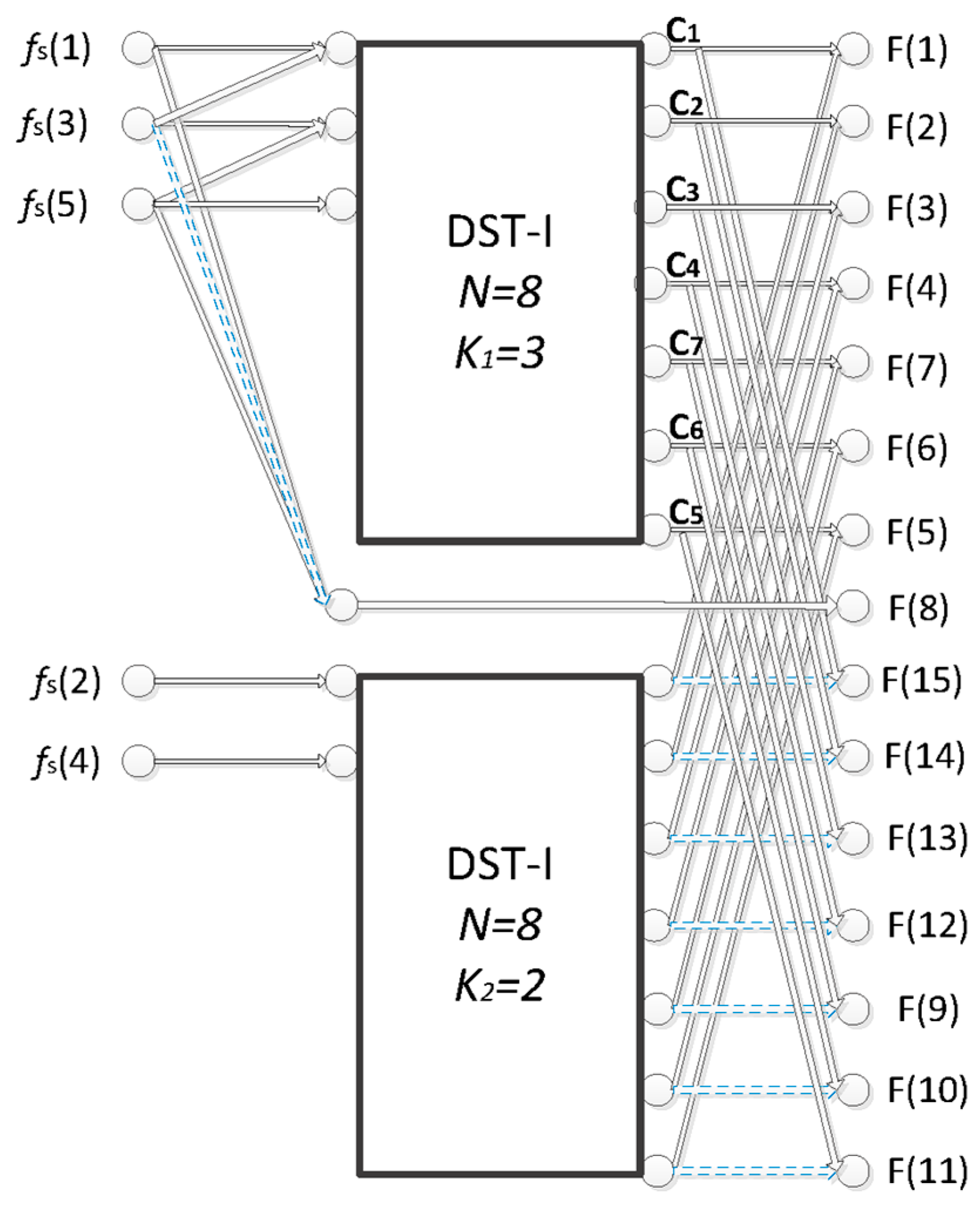
3.1. Fast-Pruned Discrete Sine Transforms

We design two fast-pruned DSTs that will be useful in the future. The sum in the first term in Equations (22) and (24) has the form:

$$F_N(s)={\displaystyle \sum _{m=1}^K{\overline{f}}_s\left(m\right){\text{sn}}_N\left(ms\right)}, s\in \left[1,N-1\right].$$

(26)

Suppose that $\left\{{\overline{f}}_s\left(m\right)=0, m>K\right\}$, $1<K<N-1$, and $s$ in ${\overline{f}}_s\left(m\right)$ is fixed; then, Equation (26) is a pruned DST of type I (DST-I). If $N$ has a power of 2, then the decimation-in-time algorithm [24] recursively splits the input DST-I into two half-length DST-I transforms with even and odd indices, as follows:

$$\begin{array}{c}{F}_N(s)=F^{}{}_{N/2}^o(s)+F^{}{}_{N/2}^e(s)\hfill \\ F_N(N-s)=F^{}{}_{N/2}^o(s)-F^{}{}_{N/2}^e(s)\hfill \end{array}, s\in [1,N/2-1].$$

(27)

where

$$\begin{array}{c}{F}^{}{}_{N/2}^o(s)=\frac{1}{2\mathrm{c}{\mathrm{s}}_N\left(s\right)}{\displaystyle \sum _{m=1}^{K_1}\left({\overline{f}}_s\left(2m-1\right)+{\overline{f}}_s\left(2m+1\right)\right)}{\mathrm{sn}}_{N/2}\left(ms\right)\hfill \\ F^{}{}_{N/2}^e(s)={\displaystyle \sum _{m=1}^{K_2}{\overline{f}}_s\left(2m\right)}{\mathrm{sn}}_{N/2}\left(ms\right)\hfill \end{array}, s\in [1,N/2-1]$$

(28)

$$F_{N/2}(N/2)={\displaystyle \sum _{m=1}^{K_1}{\overline{f}}_{N/2}\left(2m-1\right)}{\left(-1\right)}^{m+1},$$

(29)

with $K_1=\left[\left(K+1\right)/2\right]$,$K_2=\left[K/2\right]$, and [.] denotes the integer part.

This recursive procedure can be used to design a fast-pruned DST-I algorithm. Figure 1 shows a flow graph for $N= 16$ and $K=5$.

Figure 1. Flow graph of a fast-pruned DST-I algorithm, N = 16 and K = 5.

The solid and dashed blue lines represent transfer factors of 1 and −1, respectively. A circle indicates the addition if more than one input line is on the left. $C_s$ on the graph means multiplication by the coefficient $C_s=\frac{1}{2\mathrm{c}{\mathrm{s}}_N\left(s\right)}$.

The computational complexity of the pruned DST-I algorithm with respect to additions and multiplications can be estimated recursively: $C_{ADD\_DST-I}\left(N,K\right)=N/2+C_{ADD\_DST-I}\left(N/2,K_1\right)+C_{ADD\_DST-I}\left(N/2,K_2\right)+K_1-2$ and $C_{MUL\_DST-I}\left(N,K\right)=N/2+C_{MUL\_DST-I}\left(N/2,K_1\right)+C_{MUL\_DST-I}\left(N/2,K_2\right)-1$, respectively. Here, the initial condition for the computational complexity is given as $C_{ADD\_DST-I}\left(N,1\right)=0, C_{MUL\_DST-I}\left(N,1\right)=N/2-1$.

Consider the sum in the first term in Equations (23) and (25), which can be written as

$$F_N(s)={\displaystyle \sum _{m=1}^K{\overline{f}}_s\left(m\right){\mathrm{sn}}_N\left(m\left(s-1/2\right)\right)}, s\in \left[1,N\right].$$

(30)

Similarly, for $1<K<N-1$ and fixed $s$ in ${\overline{f}}_s\left(m\right)$, this is a pruned DST of type III (DST-III). If $N$ has a power of 2, then the decimation-in-time algorithm [24] recursively decomposes the input DST-III into two half-length DST-III transforms as follows:

$$\begin{array}{c}{F}_N(s)=F^{}{}_{N/2}^o(s)+F^{}{}_{N/2}^e(s)\hfill \\ F_N(N-s+1)=F^{}{}_{N/2}^o(s)-F^{}{}_{N/2}^e(s)\hfill \end{array} , s\in [1,N/2].$$

(31)

where

$$\begin{array}{c}{F}^{}{}_{N/2}^o(s)=\frac{1}{2\mathrm{c}{\mathrm{s}}_{2N}\left(2s-1\right)}{\displaystyle \sum _{m=1}^{K_1}\left({\overline{f}}_s\left(2m-1\right)+{\overline{f}}_s\left(2m+1\right)\right)}{\mathrm{sn}}_{N/2}\left(m\left(s-1/2\right)\right)\hfill \\ F^{}{}_{N/2}^e(s)={\displaystyle \sum _{m=1}^{K_2}{\overline{f}}_s\left(2m\right)}{\mathrm{sn}}_{N/2}\left(m\left(s-1/2\right)\right)\hfill \end{array}, s\in [1,N/2]$$

(32)

with $K_1=\left[\left(K+1\right)/2\right]$,$K_2=\left[K/2\right]$.

A flow graph of the fast-pruned DST-III algorithm designed on the basis of Equations (30)–(32) is shown in Figure 2, $N= 16$ and $K=5$. $C_s$ means multiplication by the coefficient $C_s=\frac{1}{2\mathrm{c}{\mathrm{s}}_{2N}\left(2s-1\right)}$.

Figure 2. Flow graph of a fast-pruned DST-III algorithm, N = 16 and K = 5.

The computational complexity of the pruned DST-III algorithm with respect to additions and multiplications can be also estimated with the following recursive equations: $C_{ADD\_DST-III}\left(N,K\right)=N/2+C_{ADD\_DST-III}\left(N/2,K_1\right)+C_{ADD\_DST-III}\left(N/2,K_2\right)$ and $C_{MUL\_DST-III}\left(N,K\right)=N/2+C_{MUL\_DST-III}\left(N/2,K_1\right)+C_{MUL\_DST-III}\left(N/2,K_2\right)$, respectively. The initial condition is given as $C_{ADD\_DST-III}\left(N,1\right)=0, C_{MUL\_DST-III}\left(N,1\right)=N/2.$

3.2. Fast Generalized Sliding Sinusoidal Transforms

To use the designed fast-pruned algorithms, we first decompose $f_s\left(k\right)$ given in Table 1 into components that do not depend on $s$ (see Table 3).

Table 3. Decomposition of $f_s\left(k\right)$ into s-independent components.

Transforms	$\mathit{s}$	Components
SCT-I	even	$f_e^1\left(k\right)=x\left(k-N_1\right)+x\left(k+N_2+2\right);f_e^2\left(k\right)=-x\left(k-N_1+1\right)-x\left(k+N_2+1\right)$
	odd	$f_o^1\left(k\right)=x\left(k-N_1\right)-x\left(k+N_2+2\right);f_o^2\left(k\right)=x\left(k+N_2+1\right)-x\left(k-N_1+1\right)$
	$\left[0,\dots N\right]$	$f_s\left(k\right)=f_s^1\left(k\right)+f_s^2\left(k\right)\mathrm{c}{\mathrm{s}}_N\left(s\right)$
SCT-II	even	$f_e^1\left(k\right)=x\left(k-N_1\right)-x\left(k-N_1+1\right)+x\left(k+N_2+2\right)-x\left(k+N_2+1\right)$
	odd	$f_o^1\left(k\right)=x\left(k-N_1\right)-x\left(k-N_1+1\right)-x\left(k+N_2+2\right)+x\left(k+N_2+1\right)$
	$\left[0,\dots N-1\right]$	$f_s\left(k\right)=f_s^1\left(k\right)\mathrm{c}{\mathrm{s}}_{2N}\left(s\right)$
SCT-III	even	$f_e^1\left(k\right)=x\left(k+N_2+2\right)$
	odd	$f_o^1\left(k\right)=-x\left(k+N_2+2\right)$
	$\left[0,\dots N-1\right]$	$f_s^0\left(k\right)=x\left(k-N_1\right);f_s^2\left(k\right)=-x\left(k-N_1+1\right)$$f_s\left(k\right)=f_s^0\left(k\right)+f_s^1\left(k\right)\mathrm{s}{\mathrm{n}}_N\left(s+1/2\right)+f_s^2\left(k\right)\mathrm{c}{\mathrm{s}}_N\left(s+1/2\right)$
SCT-IV	even	$f_e^1\left(k\right)=x\left(k+N_2+1\right)+x\left(k+N_2+2\right)$
	odd	$f_o^1\left(k\right)=-\left(k+N_2+1\right)-x\left(k+N_2+2\right)$
	$\left[0,\dots N-1\right]$	$f_s^0\left(k\right)=x\left(k-N_1\right)-x\left(k-N_1+1\right)$ $f_s\left(k\right)=f_s^0\left(k\right)\mathrm{c}{\mathrm{s}}_{2N}\left(s+1/2\right)+f_s^1\left(k\right)\mathrm{s}{\mathrm{n}}_{2N}\left(s+1/2\right)$
SST-I	even	$f_e^1\left(k\right)=x\left(k-N_1\right)-x\left(k+N_2+2\right)$
	odd	$f_o^1=x\left(k-N_1\right)+x\left(k+N_2+2\right)$
	$\left[1,\dots N-1\right]$	$f_s\left(k\right)=f_s^1\left(k\right)\mathrm{s}{\mathrm{n}}_N\left(s\right)$
SST-II	even	$f_e^1\left(k\right)=x\left(k-N_1\right)+x\left(k-N_1+1\right)-x\left(k+N_2+2\right)-x\left(k+N_2+1\right)$
	odd	$f_o^1\left(k\right)=x\left(k-N_1\right)+x\left(k-N_1+1\right)+x\left(k+N_2+2\right)+x\left(k+N_2+1\right)$
	$\left[1,\dots N\right]$	$f_s\left(k\right)=f_s^1\left(k\right)\mathrm{s}{\mathrm{n}}_{2N}\left(s\right)$
SST-III	even	$f_e^1\left(k\right)=x\left(k+N_2+1\right);f_e^2\left(k\right)=-x\left(k+N_2+2\right)$
	odd	$f_o^1\left(k\right)=-x\left(k+N_2+1\right);f_o^2\left(k\right)=x\left(k+N_2+2\right)$
	$\left[1,\dots N\right]$	$f_s^0\left(k\right)=x\left(k-N_1\right)$ $f_s\left(k\right)=f_s^0\left(k\right)\mathrm{s}{\mathrm{n}}_N\left(s-1/2\right)+f_s^1\left(k\right)\mathrm{c}{\mathrm{s}}_N\left(s-1/2\right)+f_s^2\left(k\right)$
SST-IV	even	$f_e^1\left(k\right)=x\left(k+N_2+1\right)-x\left(k+N_2+2\right)$
	odd	$f_o^1\left(k\right)=x\left(k+N_2+2\right)-x\left(k+N_2+1\right)$
	$\left[1,\dots N\right]$	$f_s^0\left(k\right)=x\left(k-N_1\right)+x\left(k-N_1+1\right)$ $f_s\left(k\right)=f_s^0\left(k\right)\mathrm{s}{\mathrm{n}}_{2N}\left(s-1/2\right)+f_s^1\left(k\right)\mathrm{c}{\mathrm{s}}_{2N}\left(s-1/2\right)$

It can be seen that $f_s^0\left(k\right)$ is s-independent, whereas each of $f_s^1\left(k\right)$ and $f_s^2\left(k\right)$ takes only two values depending on the parity of s. Using the components of $f_s\left(k\right)$, one can define $\left\{{\overline{f}}_s^i\left(m\right)=f_s^i\left(m-1\right)+f_s^i\left(2K-m-1\right) \mathrm{and} {\overline{f}}_s^i\left(K\right)=f_s^i\left(K-1\right); m=1,\dots ,K-1, i=0, 1, 2\right\}$ and express the first terms of generalized sliding sinusoidal transforms (see recursive Equations (22)–(25)) in terms of the fast-pruned DST algorithms as follows:

$$\begin{array}{l}\mathrm{GSCT}-\mathrm{I}:\frac{{\displaystyle \sum _{m=1}^K{\overline{f}}_s\left(m\right){\mathrm{sn}}_N\left(ms\right)}}{{\mathrm{sn}}_N\left(s\right)}=\frac{\mathrm{DST}-\mathrm{I}\left[{\overline{f}}_s^1\left(m\right)\right]+\mathrm{c}{\mathrm{s}}_N\left(s\right)\mathrm{DST}-\mathrm{I}\left[{\overline{f}}_s^2\left(m\right)\right]}{{\mathrm{sn}}_N\left(s\right)}=\\ \frac{\mathrm{DST}-\mathrm{I}\left[{\overline{f}}_s^1\left(m\right)+\left({\overline{f}}_s^2\left(m-1\right)+{\overline{f}}_s^2\left(m+1\right)\right)/2\right]+{\overline{f}}_s^2\left(K\right){\mathrm{sn}}_N\left(\left(K+1\right)s\right)/2}{{\mathrm{sn}}_N\left(s\right)},\\ \hfill \left\{{\overline{f}}_s^2\left(K+1\right)={\overline{f}}_s^2\left(0\right)=0\right\},s\in \left[1,N-1\right];\end{array}$$

(33)

$$\mathrm{GSCT}-\mathrm{II}:\frac{{\displaystyle \sum _{m=1}^K{\overline{f}}_s\left(m\right){\mathrm{sn}}_N\left(ms\right)}}{{\mathrm{sn}}_N\left(s\right)}=\frac{1}{{2\mathrm{sn}}_{2N}\left(s\right)}\mathrm{DST}-\mathrm{I}\left[{\overline{f}}_s^1\left(m\right)\right], s\in \left[1,N-1\right];$$

(34)

$$\begin{array}{c}\text{GSCT-III}:\frac{{\displaystyle \sum _{m=1}^K{\overline{f}}_s\left(m\right){\text{sn}}_N\left(m\left(s+1/2\right)\right)}}{{\text{sn}}_N\left(s+1/2\right)}=\frac{\text{DST-III}\left[{\overline{f}}_{s+1}^0\left(m\right)\right]+\mathrm{c}{\mathrm{s}}_N\left(s+1/2\right)\text{DST-III}\left[{\overline{f}}_{s+1}^2\left(m\right)\right]}{{\text{sn}}_N\left(s+1/2\right)}\text{+}\hfill \\ \text{+DST-III}\left[{\overline{f}}_{s+1}^1\left(m\right)\right]=\frac{\text{DST-III}\left[{\overline{f}}_{s+1}^0\left(m\right)+\left({\overline{f}}_{s+1}^2\left(m-1\right)+{\overline{f}}_{s+1}^2\left(m+1\right)\right)/2\right]}{{\text{sn}}_N\left(s+1/2\right)}+\hfill \\ \frac{{\overline{f}}_{s+1}^2\left(K\right){\text{sn}}_N\left(\left(K+1\right)\left(s+1/2\right)\right)/2}{{\text{sn}}_N\left(s+1/2\right)}\text{+DST-III}\left[{\overline{f}}_{s+1}^1\left(m\right)\right], \left\{{\overline{f}}_{s+1}^2\left(K+1\right)={\overline{f}}_{s+1}^2\left(0\right)=0\right\},s\in \left[0,N-1\right];\hfill \end{array}$$

(35)

$$\begin{array}{l}\mathrm{GSCT}-\mathrm{IV}:\frac{{\displaystyle \sum _{m=1}^K{\overline{f}}_s\left(m\right){\mathrm{sn}}_N\left(m\left(s+1/2\right)\right)}}{{\mathrm{sn}}_N\left(s+1/2\right)}=\frac{1}{{2\mathrm{sn}}_{2N}\left(s+1/2\right)}\mathrm{DST}-\mathrm{III}\left[{\overline{f}}_{s+1}^0\left(m\right)\right]+\\ \hfill +\frac{1}{{2\mathrm{cs}}_{2N}\left(s+1/2\right)}\mathrm{DST}-\mathrm{III}\left[{\overline{f}}_{s+1}^1\left(m\right)\right], s\in \left[0,N-1\right];\end{array}$$

(36)

$$\mathrm{GSST}-\mathrm{I}:\frac{{\displaystyle \sum _{m=1}^K{\overline{f}}_s\left(m\right){\mathrm{sn}}_N\left(ms\right)}}{{\mathrm{sn}}_N\left(s\right)}=\mathrm{DST}-\mathrm{I}\left[{\overline{f}}_s^1\left(m\right)\right], s\in \left[1,N-1\right];$$

(37)

$$\mathrm{GSST}-\mathrm{II}:\frac{{\displaystyle \sum _{m=1}^K{\overline{f}}_s\left(m\right){\mathrm{sn}}_N\left(ms\right)}}{{\mathrm{sn}}_N\left(s\right)}=\frac{1}{{2\mathrm{cs}}_{2N}\left(s\right)}\mathrm{DST}-\mathrm{I}\left[{\overline{f}}_s^1\left(m\right)\right], s\in \left[1,N\right];$$

(38)

$$\begin{array}{c}\text{GSST-III}:\frac{{\displaystyle \sum _{m=1}^K{\overline{f}}_s\left(m\right){\text{sn}}_N\left(m\left(s-1/2\right)\right)}}{{\text{sn}}_N\left(s-1/2\right)}=\frac{\mathrm{c}{\mathrm{s}}_N\left(s-1/2\right)\text{DST-III}\left[{\overline{f}}_s^1\left(m\right)\right]+\text{DST-III}\left[{\overline{f}}_s^2\left(m\right)\right]}{{\text{sn}}_N\left(s-1/2\right)}+\hfill \\ +\text{DST-III}\left[{\overline{f}}_s^0\left(m\right)\right]\text{=}\frac{\text{DST-III}\left[{\overline{f}}_s^2\left(m\right)+\left({\overline{f}}_s^1\left(m-1\right)+{\overline{f}}_s^1\left(m+1\right)\right)/2\right]}{{\text{sn}}_N\left(s-1/2\right)}+\hfill \\ +\frac{{\overline{f}}_s^1\left(K\right){\text{sn}}_N\left(\left(K+1\right)\left(s-1/2\right)\right)/2}{{\text{sn}}_N\left(s-1/2\right)}+\text{DST-III}\left[{\overline{f}}_s^0\left(m\right)\right], \left\{{\overline{f}}_s^1\left(K+1\right)={\overline{f}}_s^1\left(0\right)=0\right\},s\in \left[1,N\right];\hfill \end{array}$$

(39)

$$\begin{array}{l}\mathrm{GSST}-\mathrm{IV}:\frac{{\displaystyle \sum _{m=1}^K{\overline{f}}_s\left(m\right){\mathrm{sn}}_N\left(m\left(s-1/2\right)\right)}}{{\mathrm{sn}}_N\left(s-1/2\right)}=\frac{1}{{2\mathrm{sn}}_{2N}\left(s-1/2\right)}\mathrm{DST}-\mathrm{III}\left[{\overline{f}}_s^1\left(m\right)\right]+\\ \hfill +\frac{1}{{2\mathrm{cs}}_{2N}\left(s-1/2\right)}\mathrm{DST}-\mathrm{III}\left[{\overline{f}}_s^0\left(m\right)\right],s\in \left[1,N\right].\end{array}$$

(40)

Here, $\mathrm{DST}-\mathrm{I}\left[v\left(m\right)\right]$ and $\mathrm{DST}-\mathrm{III}\left[v\left(m\right)\right]$ denote the fast-pruned DST-I and DST-III algorithms over the input signal $v\left(m\right)$, respectively.

Finally, by substituting Equations (33)–(40) into recursive Equations (22)–(25), we can obtain a fast implementation of all generalized sliding sinusoidal transforms. To more clearly illustrate the design of the proposed algorithms, a simple example for computing the generalized DST-I coefficients for $K=2, N_1= 7, N_2= 7$, and $N= 16$ is provided in Appendix A.

3.3. Analysis of Computational Complexity

Taking into account Equations (22)–(25) and (33)–(40), Table 3, and the complexity of fast-pruned DST-I and DST-III algorithms, the computational complexity of the proposed generalized sliding sinusoidal transforms can be estimated as shown in Table 4.

Table 4. Complexity of fast-generalized sliding sinusoidal transforms.

Transforms	$\mathbf{Number} \mathbf{of} \mathbf{Additions} {\mathit{C}}_{\mathit{A}\mathit{D}\mathit{D}-\mathit{f}}$	$\mathbf{Number} \mathbf{of} \mathbf{Multiplications} {\mathit{C}}_{\mathit{M}\mathit{U}\mathit{L}-\mathit{f}}$
GSCT-I	$3N+10K-3+C_{ADD\_DST-I}\left(N,K\right)$	$3N+4K-2+C_{MUL\_DST-I}\left(N,K\right)$
GSST-I	$2N+3K-3+C_{ADD\_DST-I}\left(N,K\right)$	$N-1+C_{MUL\_DST-I}\left(N,K\right)$
GSCT-II GSST-II	$2N+9K-3+C_{ADD\_DST-I}\left(N,K\right)$	$2N+K-2+C_{MUL\_DST-I}\left(N,K\right)$
GSCT-III GSST-III	$4N+5K-3+2C_{ADD\_DST-III}\left(N,K\right)$	$3N+2K+2C_{MUL\_DST-III}\left(N,K\right)$
GSCT-IV GSST-IV	$3N+5K-2+2C_{ADD\_DST-III}\left(N,K\right)$	$2N+2C_{MUL\_DST-III}\left(N,K\right)$

Note that the calculation of ${\overline{f}}_s^i\left(k\right)$ from $f_s^i\left(k\right)$ around time k requires the addition of $K-1$. Coefficients $\left\{f_s^i\left(k\right)\right.\left.; k=1,\dots K-1; i=0,2,3\right\}$ have already been calculated and stored at time $K$. Additional costs are also required to calculate the initial K coefficients for each $\left\{f_s^i\left(k\right)\right.\left.;i=0,2,3\right\}$.

The proposed algorithms require 2N memory locations to store the transform coefficients computed at times 0 and K. Note that no additional memory is required to store the output, as the recursive calculation is made “in-place” using the memory originally occupied by the computed coefficients at time 0. The algorithms also need $3N/2$ additional memory locations for each pruned DST for storing $F_N\left(s\right)$ and $C_s$ factors. Depending on the type of generalized sinusoidal transform, additional memory locations are required to store $f_s^i\left(k\right)$, ${\overline{f}}_s^i\left(k\right)$ and sinusoidal weights.

4. Results

Fast radix-2 algorithms are the most popular fast algorithms for computing discrete sinusoidal transforms. In this section, the performance of the proposed algorithms in terms of computational costs and execution time is compared with that of fast radix-2 algorithms when computing generalized sliding sinusoidal transforms. In addition, the computational complexity of the proposed GSCTs is compared with that of recursive generalized sliding cosine algorithms [22].

Table 5 and Table 6 show the computational complexity of the proposed algorithms in terms of additions and multiplications, respectively, when step $K$ is varied and window size N is fixed.

Table 5. Complexity of the proposed algorithms in terms of additions, N = 256.

Step K	GSCT-I	GSST-I	GSCT-II GSST-II	GSCT-III GSST-III	GSCT-IV GSST-IV
2	1039	769	781	1543	1288
3	1176	899	917	1804	1549
4	1312	1028	1052	2065	1810
5	1386	1095	1125	2198	1943
8	1604	1292	1340	2597	2342
10	1689	1363	1423	2735	2480
16	1936	1568	1664	3149	2894
32	2352	1872	2064	3741	3486
64	2962	2240	2624	4413	4158

Table 6. Complexity of the proposed algorithms in terms of multiplications, N = 256.

Step K	GSCT-I	GSST-I	GSCT-II GSST-II	GSCT-III GSST-III	GSCT-IV GSST-IV
2	1027	508	765	1284	1024
3	1093	570	828	1414	1152
4	1159	632	891	1544	1280
5	1193	662	922	1610	1344
8	1295	752	1015	1808	1536
10	1331	780	1045	1876	1600
16	1439	864	1135	2080	1792
32	1599	960	1247	2368	2048
64	1791	1024	1343	2688	2304

First, the computational complexity of the proposed GSCTs was compared with that of recursive generalized sliding cosine algorithms [22]. The complexity of the latter algorithms with respect to additions and multiplications is presented in Table 7 and Table 8, respectively.

Table 7. Complexity of recursive sliding DCT algorithms [22] in terms of additions, N = 256.

Step K	DCT-I	DCT-II	DCT-III	DCT-IV
2	2295	1275	2304	2304
3	3315	1785	3328	3328
4	4335	2295	4352	4352
5	5355	2805	5376	5376
8	8415	4335	8448	8448
10	10,455	5355	10,496	10,496
16	16,575	8415	16,640	16,640
32	32,895	16,575	33,024	33,024
64	65,535	32,895	65,792	65,792

Table 8. Complexity of recursive sliding DCT algorithms [22] in terms of multiplications, N = 256.

Step K	DCT-I	DCT-II	DCT-III	DCT-IV
2	2304	1288	2304	2304
3	3328	1804	3328	3328
4	4352	2320	4352	4352
5	5376	2836	5376	5376
8	8448	4384	8448	8448
10	10,496	5416	10,496	10,496
16	16,640	8512	16,640	16,640
32	33,024	16,768	33,024	33,024
64	65,792	33,280	65,792	65,792

One can observe that the proposed GSCTs are superior to the corresponding recursive generalized sliding cosine algorithms.

Next, the performance of the proposed algorithms was compared with that of fast radix-2 DCT and DST algorithms. The computational complexity of common fast radix-2 DCT/DST algorithms with respect to additions and multiplications is listed in Table 9.

Table 9. Complexity of fast DCT/DST algorithms in terms of additions/multiplications; N = 256.

Operations	FDCT-I [25]	FDST-I [26]	FDCT-II [27] FDST-II [26]	FDCT-III [28] FDST-III [26]	FDCT-IV [25]	FDST-IV [26]
ADD	2716	2554	2818	2818	3456	3072
MUL	917	769	1025	1025	1664	1280

It can be seen that the proposed algorithms GCST-I, GSST-I, GCST-II, GSST-II, GCST-IV, and GSST-IV outperform the corresponding fast algorithms for a wide range of parameter K. The proposed algorithms GCST-III and GSST-III are only efficient for small K values.

Table 10 and Table 11 show how the computational complexity with respect to additions and multiplications changes as window size N varies and K is fixed. It can be seen that, as window size N increases, the gain in the proposed algorithms increases in terms of computational complexity.

Table 10. Complexity of the proposed algorithms in terms of additions, K = 16.

N	GSCT-I	GSST-I	GSCT-II GSST-II	GSCT-III GSST-III	GSCT-IV GSST-IV
32	368	224	320	461	430
64	592	416	512	845	782
128	1040	800	896	1613	1486
256	1936	1568	1664	3149	2894
512	3728	3104	3200	6221	5710
1024	7312	6176	6272	12,365	11,342
2048	14,480	12,320	12,416	24,653	22,606

Table 11. Complexity of the proposed algorithms in terms of multiplications, K = 16.

N	GSCT-I	GSST-I	GSCT-II GSST-II	GSCT-III GSST-III	GSCT-IV GSST-IV
32	207	80	127	288	224
64	383	192	271	544	448
128	738	416	559	1056	896
256	1439	864	1135	2080	1792
512	2847	1760	2287	4128	3584
1024	5643	3552	4591	8224	7168
2048	11,295	7136	9199	16,416	14,336

The actual running time of an algorithm depends on the hardware and software characteristics and the specific implementation of the algorithm. The purpose of the following simulation was to demonstrate that the theoretical computational complexity of the tested algorithms closely correlates with the execution time of the implemented algorithms. All the tested algorithms were implemented on a laptop with an Intel Core i7-2630QM processor and 8 GB RAM using MATLAB R2016a.

All the experiments were repeated 100 times to ensure statistically correct results, and the average runtime results for each algorithm were calculated. Figure 3 and Figure 4 show the runtime performance of the proposed GSCT-I, GCST-II, GCST-III, GCST-IV, and corresponding fast radix-2 algorithms.

Figure 3. Running time (milliseconds) of the tested DCT-I and DCT-II algorithms per window when N = 256 and K varies.

Figure 4. Running time (milliseconds) of the tested DCT-III and DCT-IV algorithms per window when N = 256 and K varies.

Considering that floating-point addition and multiplication in modern processors are comparable in terms of execution time, we can observe that the theoretical results presented in Table 5, Table 6 and Table 9 are in good agreement with the experimental results in Figure 3 and Figure 4.

5. Conclusions

A generalized solution of a second-order linear nonhomogeneous difference equation was derived. Based on the generalized solution, eight generalized sliding sinusoidal transforms are proposed. Fast algorithms were developed to compute generalized sliding sinusoidal transforms. The algorithms were based on the derived recursive equations and designed fast-pruned DSTs. The performance of the proposed algorithms in terms of computational complexity and execution time was compared with that of recursive generalized sliding cosine transforms and fast discrete sinusoidal algorithms. GCST-I, GSST-I, GCST-II, GSST-II, GCST-IV, and GSST-IV outperformed the corresponding fast algorithms for a wide range of parameters. It was also shown that the obtained theoretical results were in good agreement with the experimental results.

References

1. Jain, A.K. A fast Karhunen-Loeve transform for a class of random processes. IEEE Trans. Commun. 1976, 24, 1023–1029. [Google Scholar] [CrossRef]
2. Jain, A.K. A sinusoidal family of unitary transforms. IEEE Trans. Pattern Anal. Mach. Intell. 1979, PAMI-1, 356–365. [Google Scholar] [CrossRef]
3. Rose, K.; Heiman, A.; Dinstein, I. DCT/DST alternate-transform image coding. IEEE Trans. Commun. 1990, 38, 94–101. [Google Scholar] [CrossRef]
4. Lee, J.; Un, C. Performance of transform-domain LMS adaptive digital filters. IEEE Trans. Acoust. Speech Signal Process. 1986, 34, 499–510. [Google Scholar] [CrossRef]
5. Kober, V. Robust and efficient algorithm of image enhancement. IEEE Trans. Consum. Electron. 2006, 52, 655–659. [Google Scholar] [CrossRef]
6. Wang, Z.; Wang, L. Interpolation using the fast discrete sine transform. Signal Process. 1992, 26, 131–137. [Google Scholar] [CrossRef]
7. Kim, M.; Lee, Y.-L. Discrete sine transform-based interpolation filter for video compression. Symmetry 2017, 9, 257. [Google Scholar] [CrossRef]
8. Oppenheim, A.V.; Schafer, R.W. Discrete-Time Signal Processing, 3rd ed.; Prentice-Hall: Upper Saddle River, NJ, USA, 2009. [Google Scholar]
9. Sharma, R.R.; Kumar, M.; Pachori, R.B. Joint time-frequency domain-based CAD disease sensing system using ECG signals. IEEE Sensors J. 2019, 19, 3912–3920. [Google Scholar] [CrossRef]
10. Portnoff, M. Short-time Fourier analysis of sampled speech. IEEE Trans. Acoust. Speech Signal Process. 1981, 29, 364–373. [Google Scholar] [CrossRef]
11. Shi, J.; Zheng, J.; Liu, X.; Xiang, W.; Zhang, Q. Novel short-time fractional Fourier transform: Theory, implementation, and applications. IEEE Trans. Signal Process. 2020, 68, 3280–3295. [Google Scholar] [CrossRef]
12. Wang, X.; Huang, G.; Zhou, Z.; Tian, W.; Yao, J.; Gao, J. Radar emitter recognition based on the energy cumulant of short-time Fourier transform and reinforced deep belief network. Sensors 2018, 18, 3103. [Google Scholar] [CrossRef]
13. Wang, Y.; Veluvolu, K.C. Time-frequency analysis of non-stationary biological signals with sparse linear regression based Fourier linear combiner. Sensors 2017, 17, 1386. [Google Scholar] [CrossRef]
14. Thalmayer, A.; Zeising, S.; Fischer, G.; Kirchner, J. A robust and real-time capable envelope-based algorithm for heart sound classification: Validation under different physiological conditions. Sensors 2020, 20, 972. [Google Scholar] [CrossRef]
15. Priyadarshini, M.S.; Krishna, D.; Kumar, K.V.; Amaresh, K.; Goud, B.S.; Bajaj, M.; Altameem, T.; El-Shafai, W.; Fouda, M.M. Significance of harmonic filters by computation of short-time Fourier transform-based time–frequency representation of supply voltage. Energies 2023, 16, 2194. [Google Scholar] [CrossRef]
16. Park, C.; Ko, S. The hopping discrete Fourier transform. IEEE Signal Process. Mag. 2014, 31, 135–139. [Google Scholar] [CrossRef]
17. Kober, V. Fast recursive computation of sliding DHT with arbitrary step. Sensors 2020, 20, 5556. [Google Scholar] [CrossRef]
18. Kober, V. Fast hopping discrete sine transform. IEEE Access 2021, 9, 94293–94298. [Google Scholar] [CrossRef]
19. Xi, J.; Chiraro, J.F. Computing running DCT’s and DST’s based on their second-order shift properties. IEEE Trans. Circuits Syst. I 2000, 47, 779–783. [Google Scholar] [CrossRef]
20. Kober, V. Fast algorithms for the computation of sliding discrete sinusoidal transforms. IEEE Trans. Signal Process. 2004, 52, 1704–1710. [Google Scholar] [CrossRef]
21. Kober, V. Recursive algorithms for computing sliding DCT with arbitrary step. IEEE Sensors 2021, 21, 11507–11513. [Google Scholar] [CrossRef]
22. Qian, L.; Luo, S.; He, S.; Chen, G. Recursive algorithms for direct computation of generalized sliding discrete cosine transforms. In Proceedings of the 3rd International Congress on Image and Signal Processing, Yantai, China, 16–18 October 2010; pp. 3017–3020. [Google Scholar] [CrossRef]
23. Wang, Z. Fast algorithms for the discrete W transform and for the discrete Fourier transform. IEEE Trans. Acoust. Speech Signal Process. 1984, 32, 803–816. [Google Scholar] [CrossRef]
24. Yip, P.; Rao, K.R. Fast decimation-in-time algorithms for a family of discrete sine and cosine transforms. Circuits Syst. Signal Process. 1984, 3, 387–408. [Google Scholar] [CrossRef]
25. Hou, H.S. A fast recursive algorithm for computing the discrete cosine transform. IEEE Trans. Acoust. Speech Signal Process. 1987, 35, 1455–1461. [Google Scholar] [CrossRef]
26. Wang, Z. Fast discrete sine transform algorithms. Signal Process. 1990, 19, 91–102. [Google Scholar] [CrossRef]
27. Britanak, V. On the discrete cosine computation. Signal Process. 1994, 40, 183–194. [Google Scholar] [CrossRef]
28. Britanak, V. A unified discrete cosine and sine transform computation. Signal Process. 1995, 43, 333–339. [Google Scholar] [CrossRef]