Article

Controlling COVID-19 Spreading: A Three-Level Algorithm

by
Giovanni Dieguez
1,†,
Cristiane Batistela
2,† and
José R. C. Piqueira
1,*
1
Department of Telecommunications and Control Engineering, São Paulo, Polytechnic School, University of São Paulo, São Paulo 05508900, Brazil
2
Center for Mathematics, Computing and Cognition, Federal University of ABC, São Bernardo do Campo, São Paulo 09606070, Brazil
*
Author to whom correspondence should be addressed.
These authors contributed equally to this work.
Mathematics 2023, 11(17), 3766; https://doi.org/10.3390/math11173766
Submission received: 22 June 2023 / Revised: 23 August 2023 / Accepted: 28 August 2023 / Published: 1 September 2023
(This article belongs to the Special Issue Mathematical Modeling and Data Science for Biology and Medicine)

Abstract

:
As the main methods of the coronavirus disease (COVID-19) transmission are air and physical contact, actions to mitigate and suppress its spread must be developed in order to change population dynamics and provide efficient control strategies. Here, these actions are described as a simple heuristic framework to establish public policies. Two control systems were studied: the first organized in the form of an algorithm stratified into three levels and the second as a minimization problem similar to optimal control strategies, applied to both social distancing and vaccination. The possible effects of these actions are modeled and applied to an extension of the Susceptible - Infected - Removed (SIR) compartmental model. The control system is developed, which is organized in the form of an algorithm stratified into three levels. These levels intend to represent social distancing strategies implemented by sanitary authorities around the globe, representing stronger or weaker grades of isolation intensity according to the ability of the healthcare system to cope with symptomatic individuals. The algorithm control is applied in a simulation, and the results give evidence of the effectiveness of the procedures adopted against the coronavirus. The model dynamics are analyzed and validated with simulations considering parameters obtained from epidemiological data from Brazil and Uruguay and in a more detailed way for three Brazilian states: São Paulo, Minas Gerais and Rio de Janeiro. The model was validated using cumulative data on cases and deaths. For cases of death, the results were satisfactory, while for case data, the response was reasonable, considering the possibility of adding delays or variations in parameters in the model. In addition, the effective reproduction number was proposed for the cities studied in Brazil, the result being relevant because it has a qualitative behavior similar to that published by official centers. This paper also discusses the implementation and optimization of social distancing and vaccination control strategies, considering different parameters and their effects on reducing the number of cases and deaths. Model simulations present promising results for developing strategies to attack COVID-19 dissemination.
MSC:
93C10; 37N35

1. Introduction

At the beginning of 2020, the epidemic of a new disease changed the history of humanity; it was responsible for a global health and economic crisis. COVID-19 is a new coronavirus progeny, SARS-CoV-2, first reported in Wuhan, China, on 31 December 2019 [1,2]. A few months later, a report published by the World Health Organization qualified the disease as a pandemic due to its prevalence worldwide [3].
Transmission of SARS-CoV-2 occurs predominantly through the physical transportation of contaminated droplets of secretions from an infected individual to an uninfected person, although the role of aerosol transmission and contaminated surface contact is currently unknown [4]. It is a disease with lower lethality when compared with its high transmission capacity, with the spreading aggravated by the average incubation time and due to both symptomatic and asymptomatic people being able to transmit the disease [5].
The disease has several forms of manifestation, and most patients have rapid resolution, many of whom are asymptomatic. The initial symptoms are fever, cough and breathing difficulties. However, some patients with comorbidities may develop complications [6], requiring hospitalization, intensive treatment and mechanical respiratory ventilators, provoking a severe crisis in the healthcare system caused by excessive hospitalizations.
Different interventions aimed to slow the rapid evolution of the pandemic were adopted by many countries to avoid overcrowded hospitals. Strategies such as isolation of infected patients, mask-wearing, regular hand hygiene, social distancing, quarantine and total blocking of areas [7,8,9,10] were adopted worldwide.
Another public strategy may be associated with the impact of advertisements on social networks in combating the pandemic, in which it can be assumed that awareness among susceptible individuals alters collective behaviors, resulting in a reduction in the transmission of this infectious agent [11] or community awareness and global information campaigns [12].
Mathematical models are used to simulate the transmission of coronavirus and are helpful to understanding the dynamical behavior of an infection, providing tools to estimate the duration and peaks of infection outbreaks and designing efficient control strategies [13,14,15]. Epidemic mathematical models are present in public health literature [16,17] related to several diseases [18,19,20,21,22,23,24,25,26].
Macroscopic compartmental models for disease spreading that have been a field of research since the Kermack and McKendrick proposition [27,28,29], with a dynamic model that classifies population individuals into groups such as Susceptible - Infected - Removed (SIR) or Susceptible - Exposed - Infected - Removed (SEIR) models, could be refined by contact tracing and hospitalization strategies to explain the COVID-19 outbreak [30]. Several modifications of the SIR model [31,32,33] have been proposed for epidemic modeling [34,35,36,37], which have been useful to public health policy makers [38].
More complex mathematical models using the stochastic approach and estimating data based on outbreak probability have been studied for cases in Wuhan and other [39] locations. Another compartmental model proposed for case studies in India studied the dynamics of disease propagation and predicts [40] outbreaks, yet for that country, the control theory provides ideal strategies to maintain the disease outbreak [41]. Compartmental models that address mitigation strategies for the transmission of COVID-19 beyond social distancing, including blocking and closing educational institutions, are also studied in countries such as Italy [42]. There are still models that consider the influence of environmental contamination to investigate the dynamics of viral propagation [43].
Due to the urgency of COVID-19, researchers worldwide accepted the challenge of outlining mathematical models for this new epidemic. Several mathematical models have already been formulated for the population dynamics of COVID-19 in several countries [10,44,45,46,47,48,49,50,51], and pioneer methods are structured upon machine learning and statistical models, such as decision trees and linear regression [52] or even more powerful ones like artificial neural networks [53,54], showing promising results. Machine learning has also been used to assist in early detection [55] and prediction of severity [56] of COVID-19.
However, this paper considers a more classical and established approach, using the adjustment of social contact rate characterized by the control of the parameter β to mitigate COVID-19 spread. For this, a three-level controller is implemented and its relationship to social distance validated. An extension of the compartmental SIR model is considered, the Susceptible–Infected–Removed–Dead (SIRD) model, and the method is inspired by how control theory can help us reduce COVID-19 propagation [57].
This article’s main motivation is the study of strategies to control the spread of the SARS-CoV-2 virus and, for that, it considers public policies based on social distancing and vaccination. This work is validated with cumulative data on cases and deaths from some regions. In addition, the basal reproduction number and the effective reproduction number are calculated and compared with data from the COVID-19 observatory.
Finally, the implementation and optimization of these strategies is discussed, considering different parameters and their effects in reducing the number of cases and deaths to indicate public policies concerning the health system.
The remainder of this paper is ordered as follows: In Section 2, the equations and hypothesis of the model are presented. In Section 3, the analysis of model dynamics is exhibited, the equilibrium points are determined, and the basic reproduction rate R 0 for the SIRD model is defined and analyzed with two simulations. Then, in Section 4, the model is studied for the sake of establishing a baseline for the controller, with parameters derived from Brazil and Uruguay. Section 5 presents the validation for the proposed model with more detailed data for three Brazilian states. Finally, Section 6 outlines the controller, and its effectiveness is investigated for a hypothetical scenario, followed by the control strategy results in Section 7 and the more detailed control analysis for the states of São Paulo, Minas Gerais and Riode Janeiro in Section 8. The conclusions are shown at the end, in Section 9. All simulations are performed with MATLAB Simulink [58].

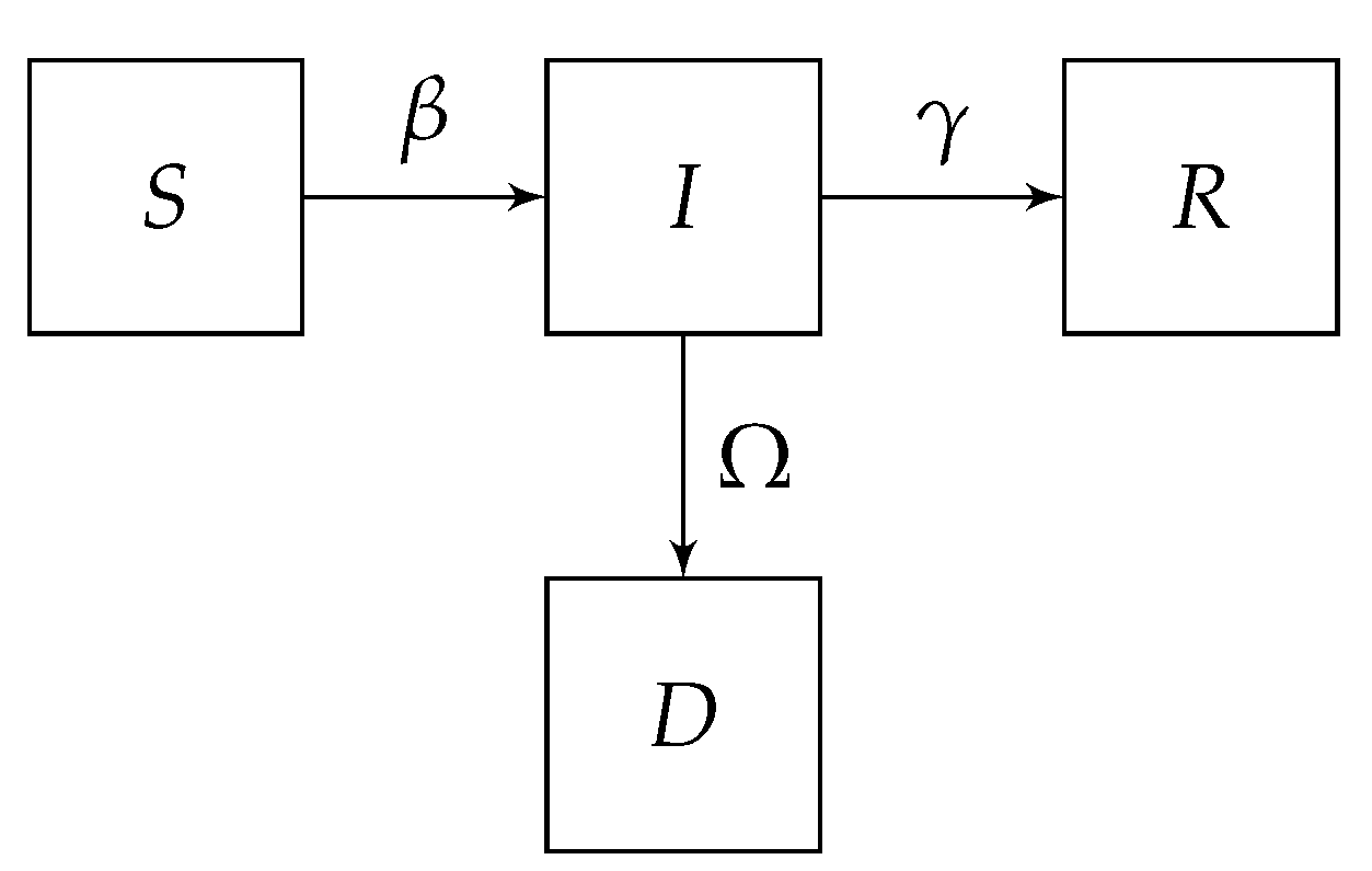
2. Model Formulation

The proposed model is a modification of the original SIR compartmental model [59], including a dead population compartment, here called the Susceptible - Infected - Removed - Dead (SIRD) model, shown in Figure 1. The model does not account for natural births and deaths, as the Dead are only due to complications caused by coronavirus infection.
Model parameters are described in Table 1. β is the average number of contacts that result in contamination, per unit of time; γ is the recovery rate, i.e., the rate at which individuals leave the infected compartment after recovering. Consequently, γ 1 represents the recovery time [60]. Additionally, Ω is the fraction of the infected population that dies per unit of time (mortality rate).
As can be observed, the model presents some simplifications:
  • A recovered individual should acquire immunity and does not return to the susceptible compartment. Hence, they become “Removed” (“R” from SIRD);
  • Parameters β , γ and Ω are considered to be constants, despite depending on individual behavior, healthcare availability and age.
Under the described conditions, the model dynamics can be written as
S ˙ = β S I N , I ˙ = β S I N ( γ + Ω ) I , R ˙ = γ I , D ˙ = Ω I .
with N = S ( t ) + I ( t ) + R ( t ) + D ( t ) and S ˙ ( t ) + I ˙ ( t ) + R ˙ ( t ) + D ˙ ( t ) = 0 .
As natural births and deaths are not taken into account, the total number of individuals in the population is considered to be constant, and the dynamics of the dead compartment can be written as a function of the other compartments:
D = N S I R , D ˙ = ( S ˙ + I ˙ + R ˙ ) .
Furthermore, the recovered compartment is dependent on the susceptible and infected populations:
R ˙ = γ γ + Ω ( S ˙ + I ˙ ) .
Therefore, the system dynamics can be rewritten without the removed and dead variables, without any loss of generality:
S ˙ = β S I N , I ˙ = β S I N ( γ + Ω ) I .

3. System Dynamics Analysis

3.1. Equilibrium Conditions

For the proposed SIRD model, equilibrium points can be obtained by applying the conditions S ˙ = 0 and I ˙ = 0 . By doing so, it can be concluded that every point of the form ( S , 0 ) is an equilibrium point.
Equilibria at I = 0 are called disease-free, as opposed to equilibria at I 0 , which are called endemic [61].

3.2. Equilibrium Points Classification

In order to analyze the local stability of these points, the Hartman–Grobman theorem is applied [62], and the general Jacobian (J) is constructed.
For ( S , I ) = ( S , 0 ) , the Jacobian is reduced to
J ( S , 0 ) = 0 β S N 0 β S N ( γ + Ω ) .
Hence, the eigenvalue set for the equilibrium points can be found by
λ ( λ β S N + γ + Ω ) = 0 ,
Which gives
( 0 , β S N ( γ + Ω ) ) ;
as the eigenvalue set. Considering that one of the eigenvalues is equal to zero, it is worth noticing that the eigenvalue set obtained from the equilibrium points allows a local stability analysis with three possibilities:
  • If β S N ( γ + Ω ) > 0 ⇒ these fixed points are unstable [62]; so, there will be a growth in cases for a small perturbation.
  • If β S N ( γ + Ω ) < 0 ⇒ the center manifold theorem must be applied in order to classify the stability condition.
Consequently, to proceed with the equilibrium stability analysis, all points satisfying β S N ( γ + Ω ) < 0 and S 0 are studied by applying the center manifold theorem.
Considering S > 0 , a new parameter τ > 0 is introduced in order to translate the system so that the point (S* = τ ,0) is the origin (0,0) of the new system. This is performed because the center manifold theorem only refers to neighborhoods of the origin of the corresponding analyzed system. Consequently, the rewritten system, with Z = S S , can be written as follows:
Z ˙ = β ( Z + τ ) I N , I ˙ = β ( Z + τ ) I N ( γ + Ω ) I .
That is, studying the system (4) around ( τ ,0) is the same as studying the new system (8) around (0,0). Nevertheless, the rewritten system does not possess the same physical interpretation as the SIRD model. In addition, substitute parameters are introduced,
ϕ = β N , α = γ + Ω ,
in order to remove nonessential parameters regarding the interpretation of the stability condition. Then,
Z ˙ = ϕ ( Z + τ ) I , I ˙ = ϕ ( Z + τ ) I α I .
Additionally, it is necessary to transform (10) into the form (A1), as shown in Appendix A, by changing the basis into a basis of eigenvectors. Consequently,
u ˙ = ( ϕ 3 τ 2 ( α ϕ τ ) 2 ϕ 2 τ α ϕ τ ) v 2 ( ϕ + ϕ 2 τ α ϕ τ ) u v , v ˙ = ( ϕ τ α ) v + ϕ u v + ϕ 2 τ α ϕ τ v 2 .
Therefore,
A = [ 0 ] , B = [ ϕ τ α ] , f ( u , v ) = ( ϕ 3 τ 2 ( α ϕ τ ) 2 ϕ 2 τ α ϕ τ ) v 2 ( ϕ + ϕ 2 τ α ϕ τ ) u v , g ( u , v ) = ϕ u v + ϕ 2 τ α ϕ τ v 2 .
To find h ( u ) , as Appendix A shows, it is necessary to consider that the coordinates of any point in the center manifold must satisfy the conditions
y = h ( x ) , | x | < δ , h ( 0 ) = 0 , D h ( 0 ) = h ˙ ( 0 ) = 0 ,
from (A2), which substituting on (A1), gives
h ˙ ( u ) [ A u + f ( u , h ( u ) ) ] = B h ( u ) + g ( u , h ( u ) ) h ˙ ( u ) [ A u + f ( u , h ( u ) ) ] B h ( u ) g ( u , h ( u ) ) = 0 .
Now, after substituting (12) (with v = h ( u ) ) into (14), it can be seen that h ( u ) = 0 is a solution to the partial differential Equation (14). Then, the vector field restricted to the center manifold is given by
u ˙ = 0 .
Therefore, u = 0 is stable in (15). Thus, Theorem A2 from Appendix A guarantees that ( Z , I ) = ( 0 , 0 ) is stable for any parameter 0 τ < N ( γ + Ω ) β and, consequently, ( S , 0 ) is stable for the same set.
To complete the stability analysis, the case with S = N ( γ + Ω ) β is considered, i.e., the center manifold theorem [62] is applied for:
  • β S N ( γ + Ω ) = 0 .
The point ( S = N ( γ + Ω ) β ,0) is the origin of the system (10) with parameter τ = α ϕ . In order to assess stability, a simulation is presented in Figure 2.
As can be seen, neighborhoods close to the origin with initial values I < 0 are unstable, as the trajectories point towards negative infinite. However, the system is only defined for I > 0 , considering that there can be no negative infected, although Z can be negative (as we translated the original system), and even a small disturbance would never take it to a point with I < 0 . Consequently, it is a degenerated equilibrium [63].

3.3. Basic Reproduction Rate

The basic reproduction rate or R 0 is defined as the average number of secondary infections produced when one infected individual is introduced into a host population, where almost everyone is susceptible ( S N ) [15,64]. For example, if the R 0 for COVID-19 in a population is 5, then each new case is expected to produce 5 secondary infections, assuming everyone around is susceptible.
Mathematically, R 0 is a threshold for stability of a disease-free equilibrium and is related to epidemic’s peak and final size [61].
Looking at the equation I ˙ from (4) it can observed that, when S N , the signal of I ˙ is defined by β ( γ + Ω ) .
Therefore, for the SIRD model, R 0 can be defined as
R 0 = β γ + Ω ,
such that, when R 0 > 1 , the equilibrium is locally unstable ( I ˙ > 0) but stable if R 0 < 1 , implying I ˙ < 0.

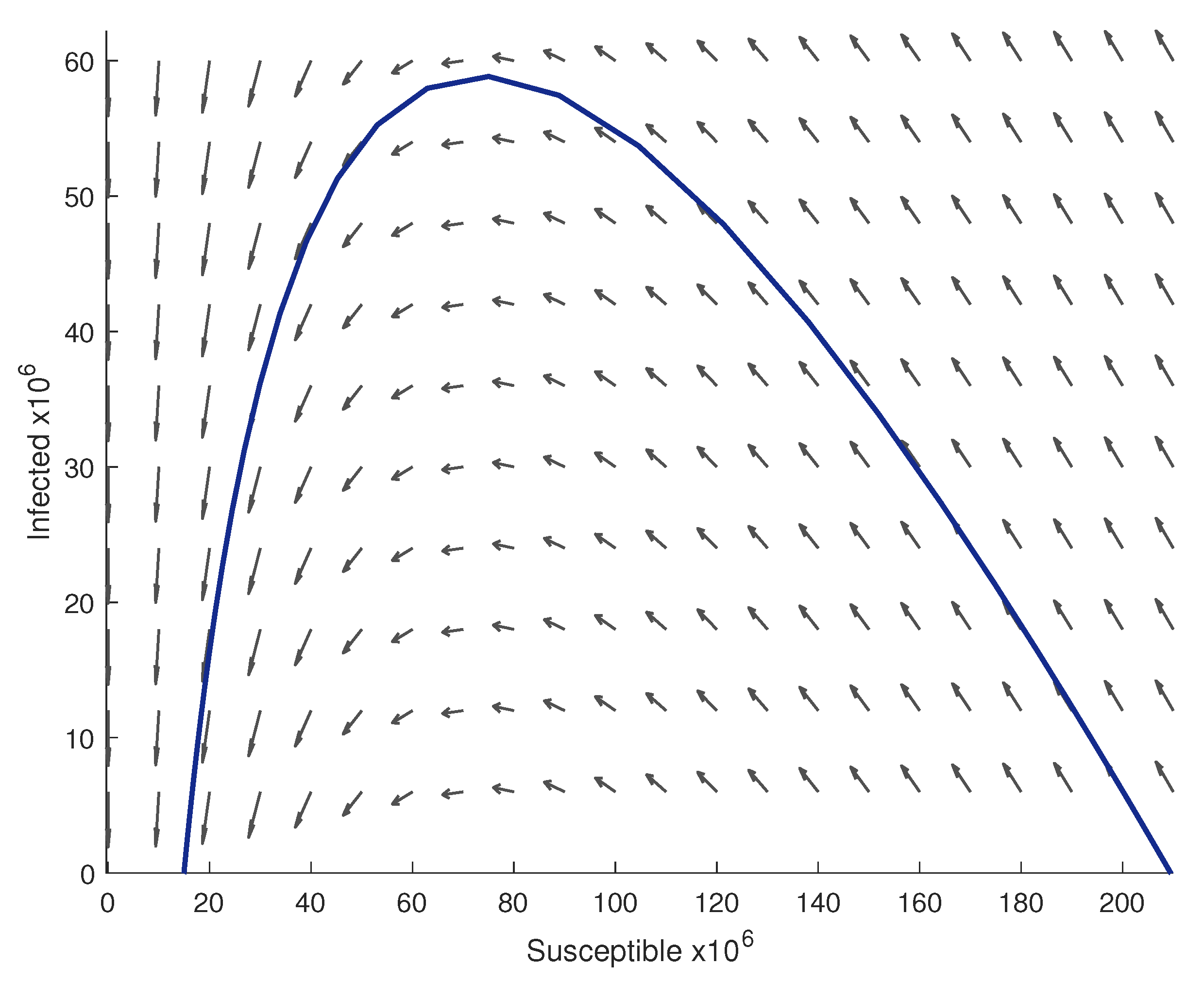
3.4. Phase Portrait for Different Values of R 0

Figure 3 and Figure 4 show the phase portrait of the system for different values of R 0 , specifically chosen to portray the only two possible outcomes.
In Figure 3, it is shown that, for R 0 > 1 , the number of infected initially grows, but, as S ˙ < 0 in that situation, at some point S N eventually becomes < 1 R 0 , which implies I ˙ < 0 , and the trajectory always ends up on the horizontal axis (I = 0). This result is known as the herd immunity value.
The interception point depends on the initial conditions. Therefore, there can be more or fewer individuals that will never become infected in the course of the epidemic (final number of susceptible at disease-free equilibrium).
In Figure 4, with R 0 < 1 , the system points toward the horizontal axis much faster, with the number of infected decreasing steeply at all times. This result is expected, as I ˙ < 0 for R 0 < 1 .

4. Case Studies and Numerical Simulations

This section presents two case studies, first with parameters derived from Brazil, followed by Uruguay. These two countries were chosen because of their different basic reproduction number, as a result of particular population dynamics concerning the contact rate β . For Brazil, R 0 is estimated to be close to 2.82 [60], and for Uruguay, R 0 is close to 1.13 [65]. These values were obtained using early infections data, as shown in Figure 5 and Figure 6, and they are believed to present a scenario where there is no response to the pandemic, both individually or systemically.
Figure 5 and Figure 6 show how the SIRD model compares with real data from Brazil and Uruguay in the early days of disease spread, with [66] as the data source.
The choice for the short time interval and period adopted is due to the emergence of the public strategy of social distancing, which was implemented at the beginning of the pandemic. In Figure 5, a smaller interval was also considered, since the data collected for Brazil are data for the country as a whole. As regions have socioeconomic and educational distinctions, they have different propagation dynamics and responses to mitigation strategies.
Both graphs display a good fitting for initial data, with subsequent detachment between model and data, which suggests there is a change in behavior due to the implementation and effectiveness of isolation policies or individual confinement. In Section 4.1, we use this set of parameters to simulate longer-term scenarios with no isolation that serve as a reference for evaluating the control algorithm.

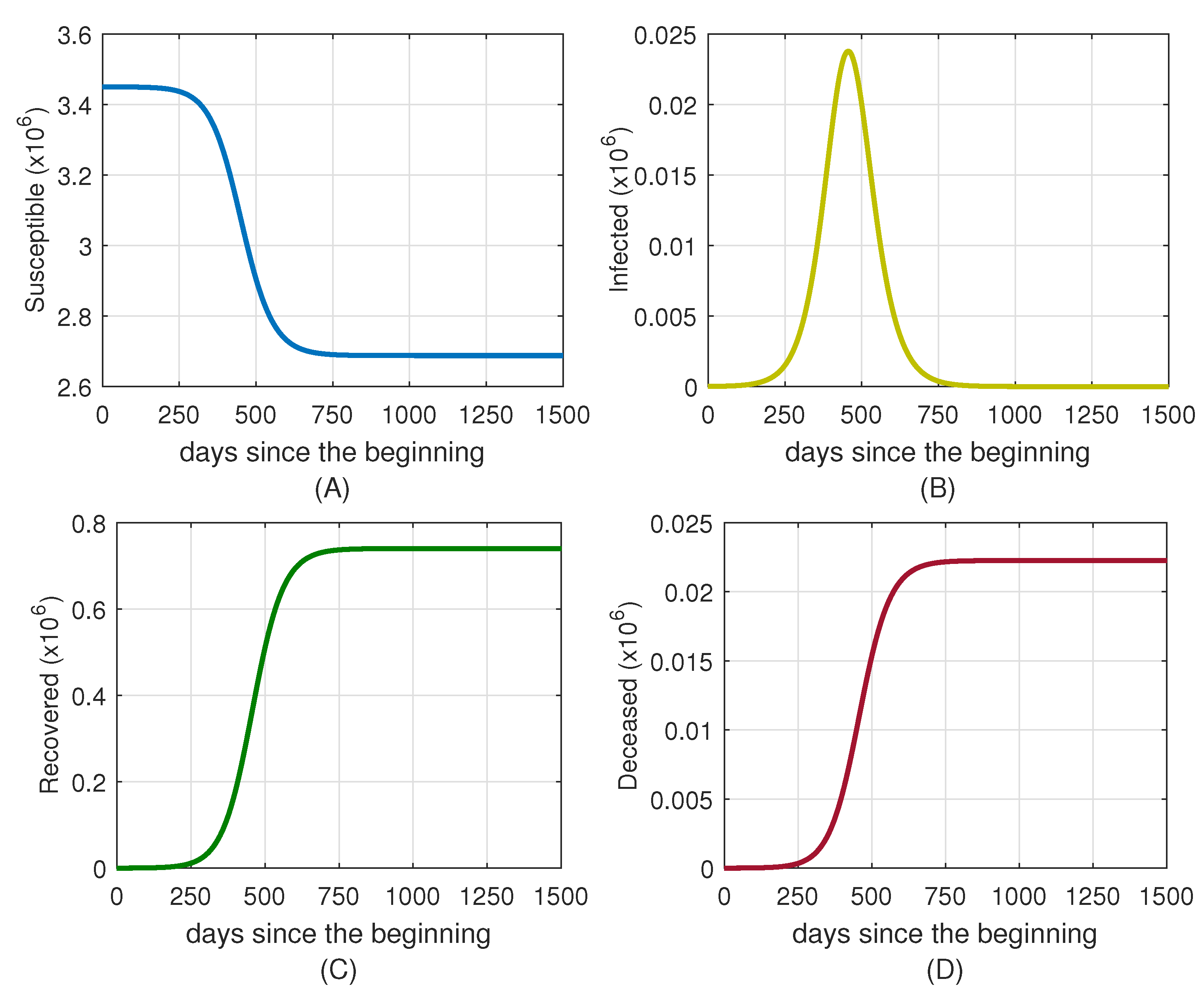
4.1. Simulation for Brazil

First, the model was simulated considering the parameters for Brazil, i.e., N = 209.5 million inhabitants, and I 0 = 10 individuals are considered, with the results shown in Figure 7.
The chosen parameters conduct a simulation for a full-blown pandemic outbreak. The last case ended about 120 days after the disease had begun being disseminated, as we can see in Figure 7B,D, which shows a high number of dead at the end, about 2.71% of the total population before the pandemic.
Figure 8 clearly shows the large proportion of the population that became infected at some point. At the end, less than 10% never became infected.

4.2. Simulation for Uruguay

The model was also simulated with parameters from Uruguay, i.e., N = 3.45 million inhabitants, considering I 0 = 10 individuals, and the results are shown in Figure 9.
As the R 0 for Uruguay is lower than Brazil’s, there is a significant difference concerning the dissemination of the virus. Figure 9 shows that the pandemic lasted much longer in Uruguay than in Brazil. However, Uruguay had much fewer dead individuals in the end, only about 0.64% of the total population before the pandemic.
The low amount of individuals that ever became infected in Uruguay is highlighted in Figure 10, which is about 24% of the total population before the pandemic. Additionally, the lower number of infected individuals suggests that having a lower R 0 due to lower β (contact rate) is a good indicator of what proportion the virus spread will achieve. This fact inspires the control algorithm used as reference for public employment polices, and it is studied in the next section.

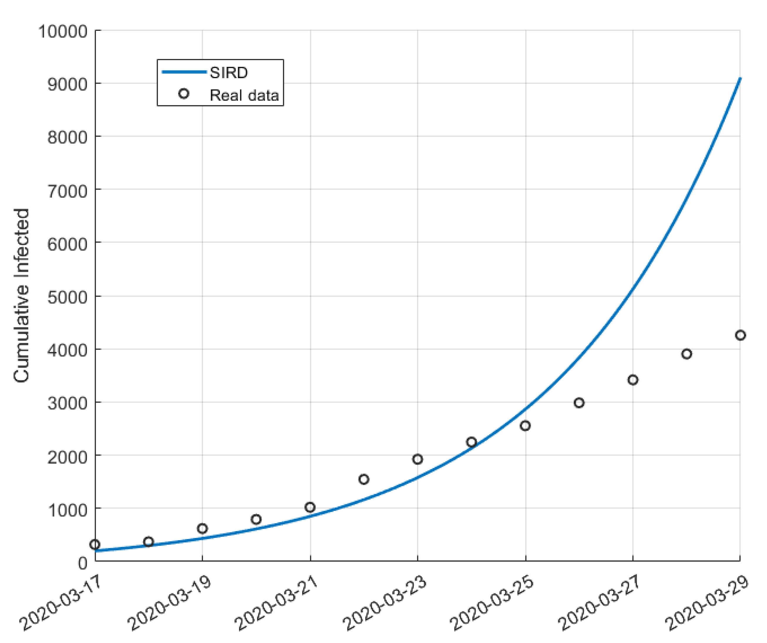
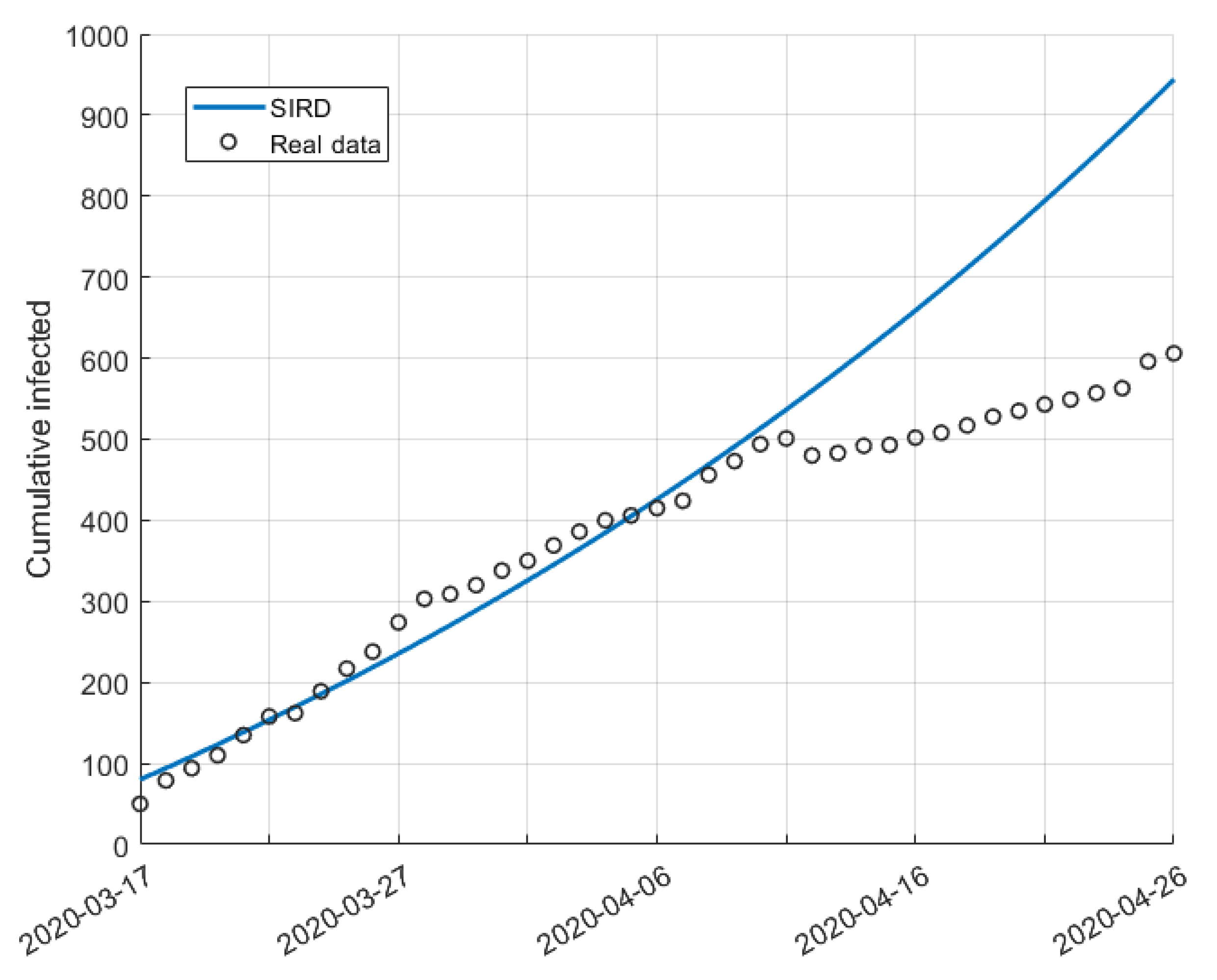
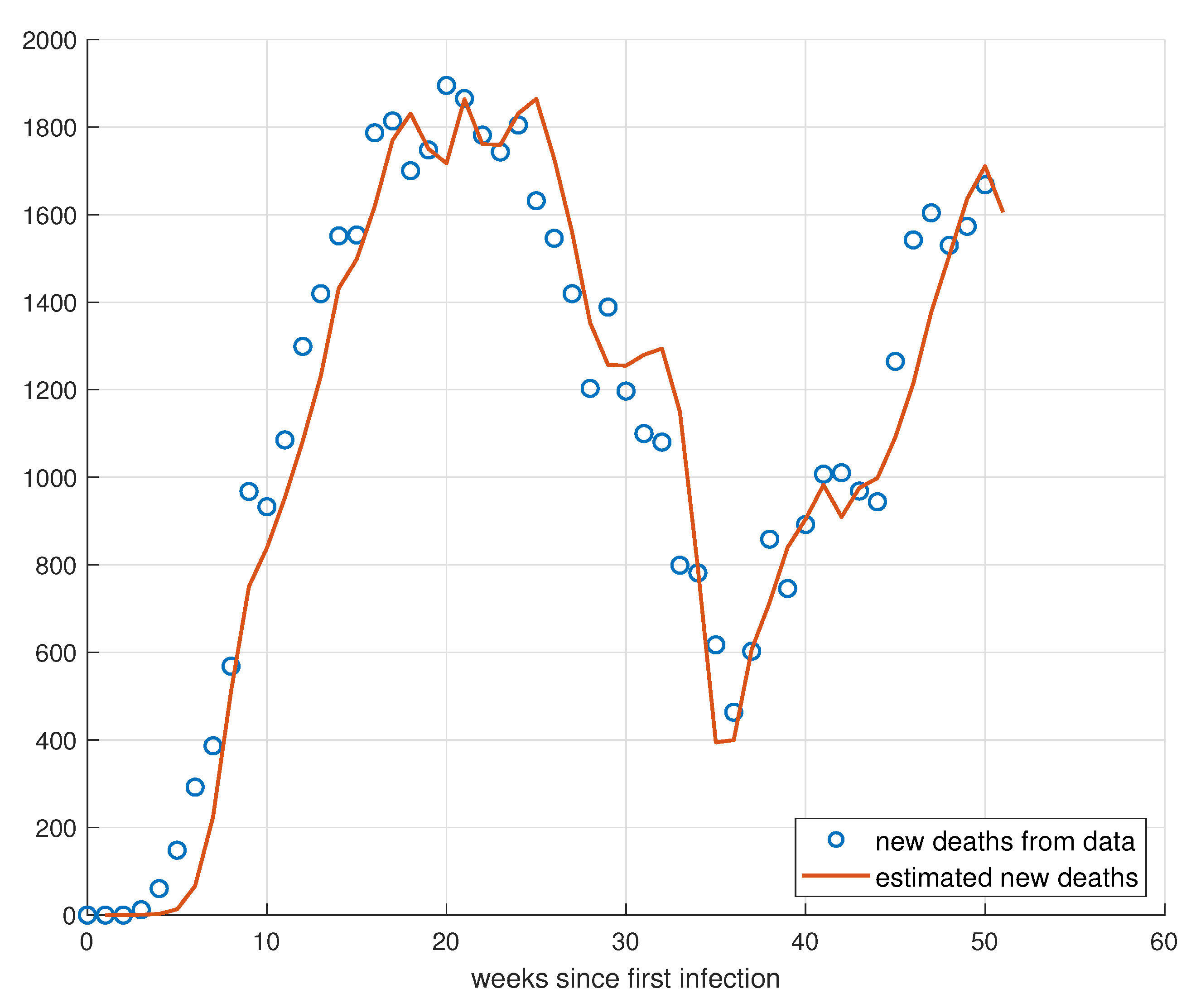
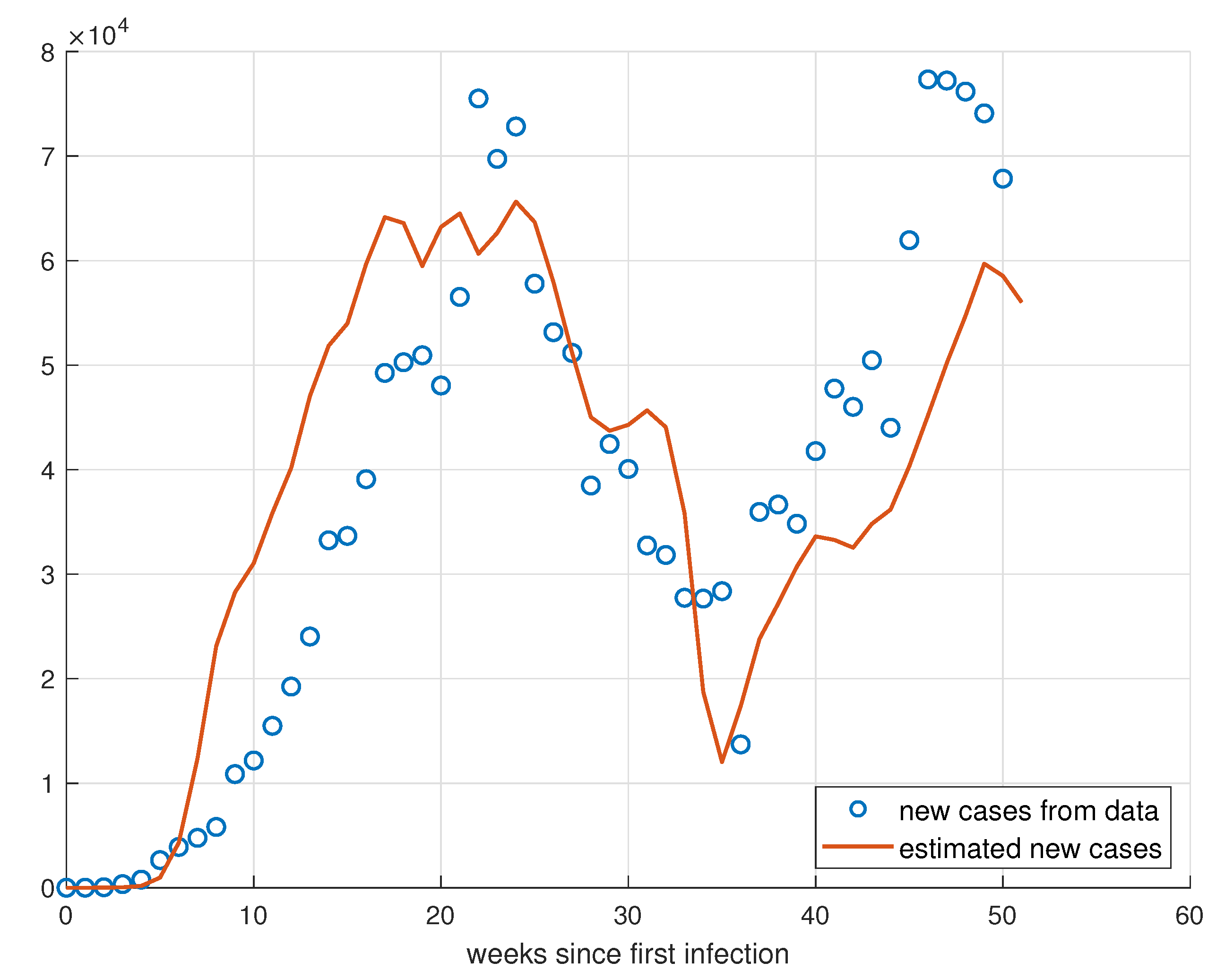
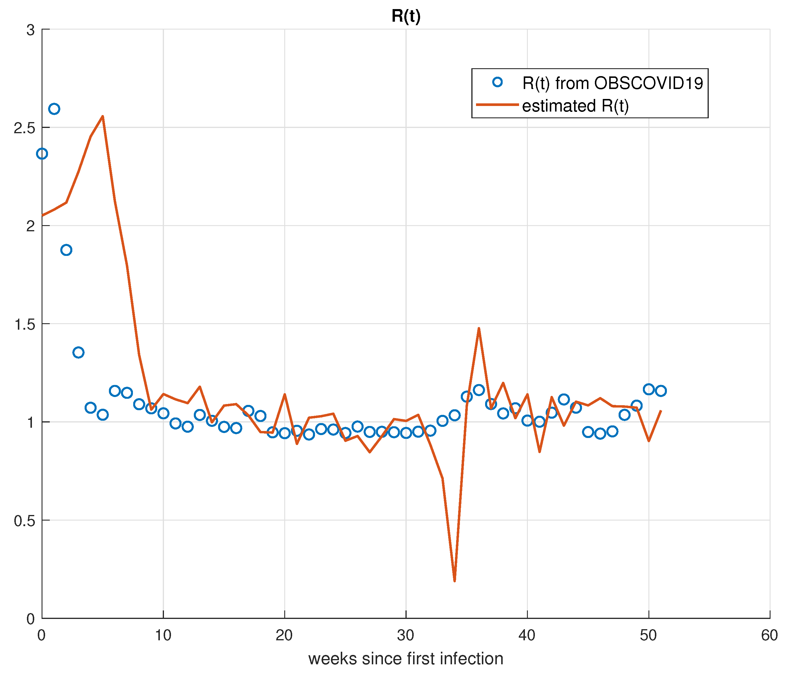
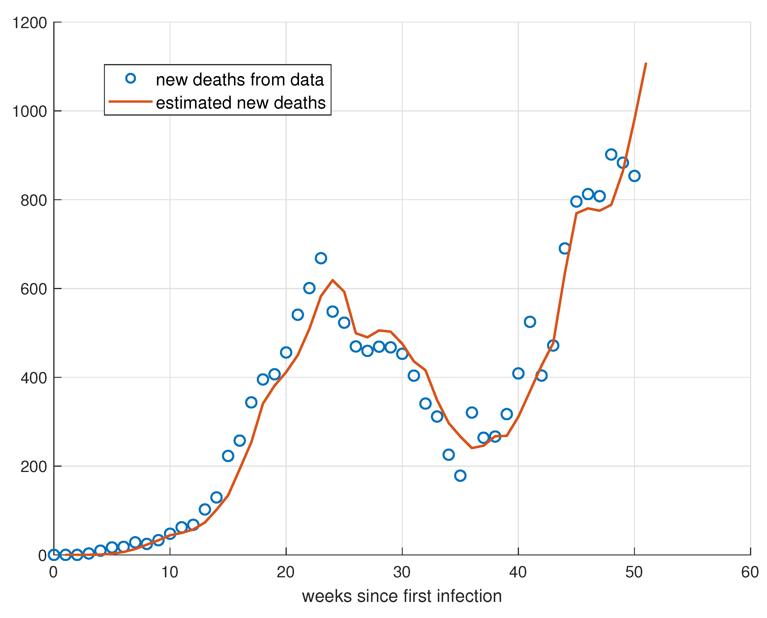
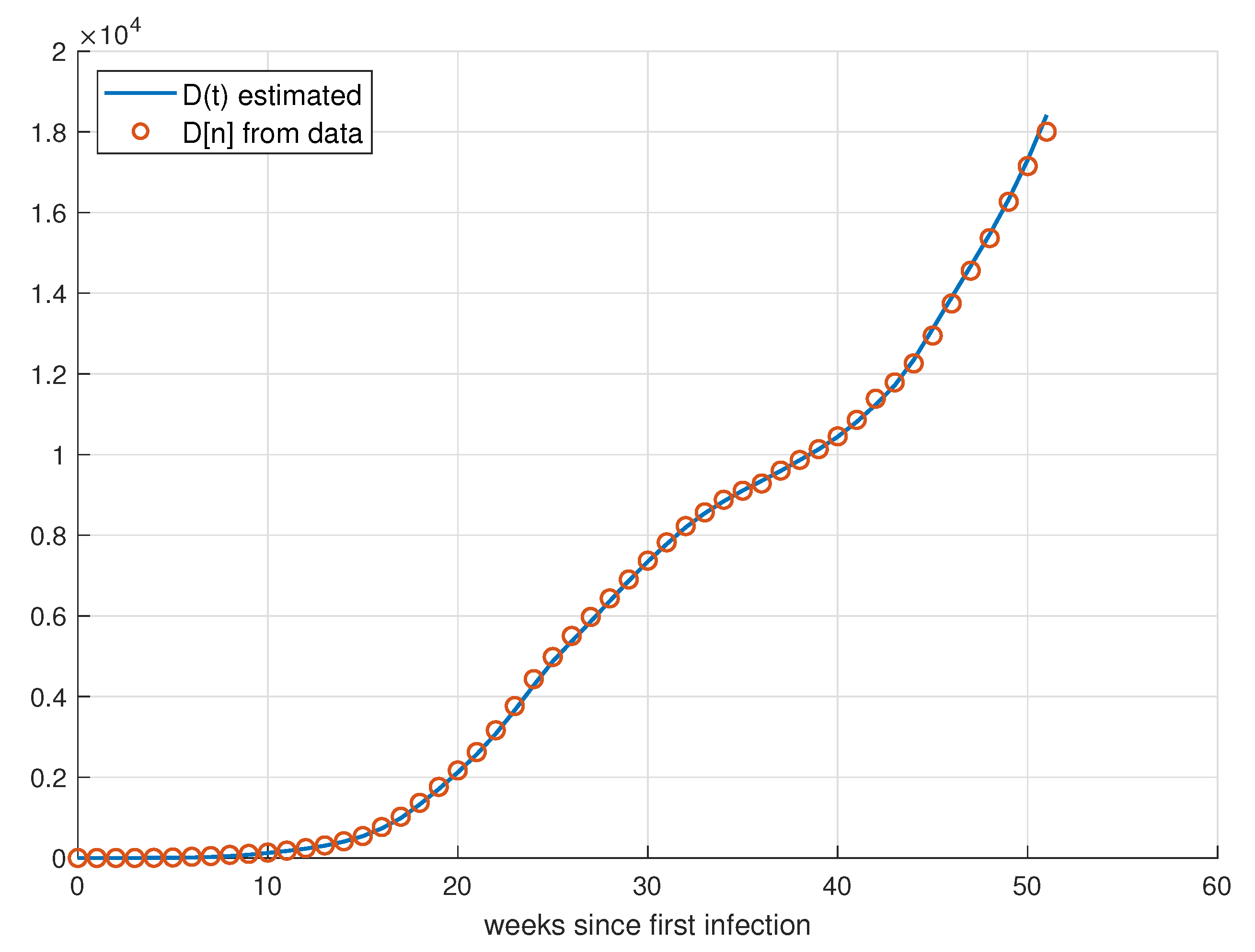
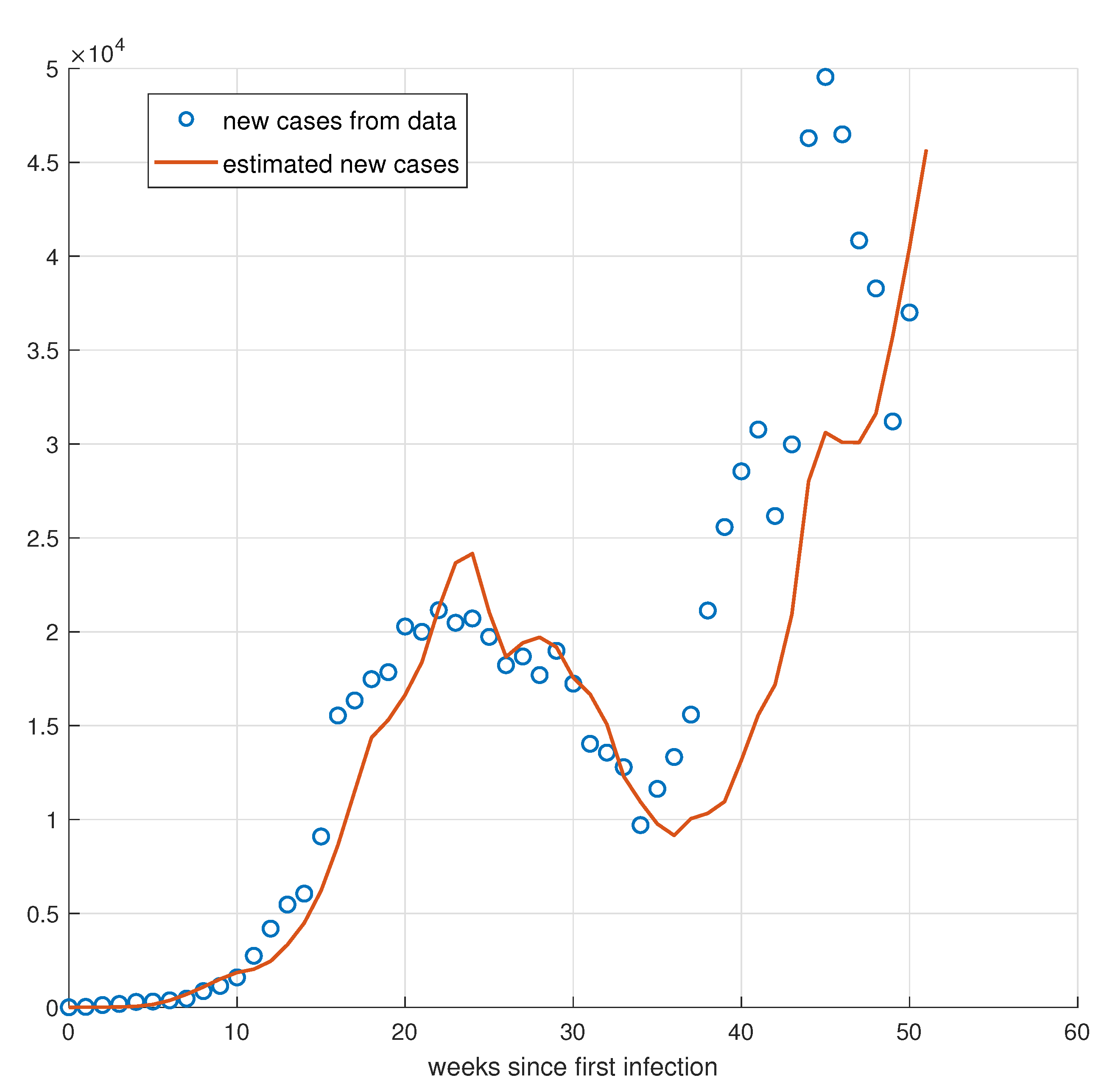
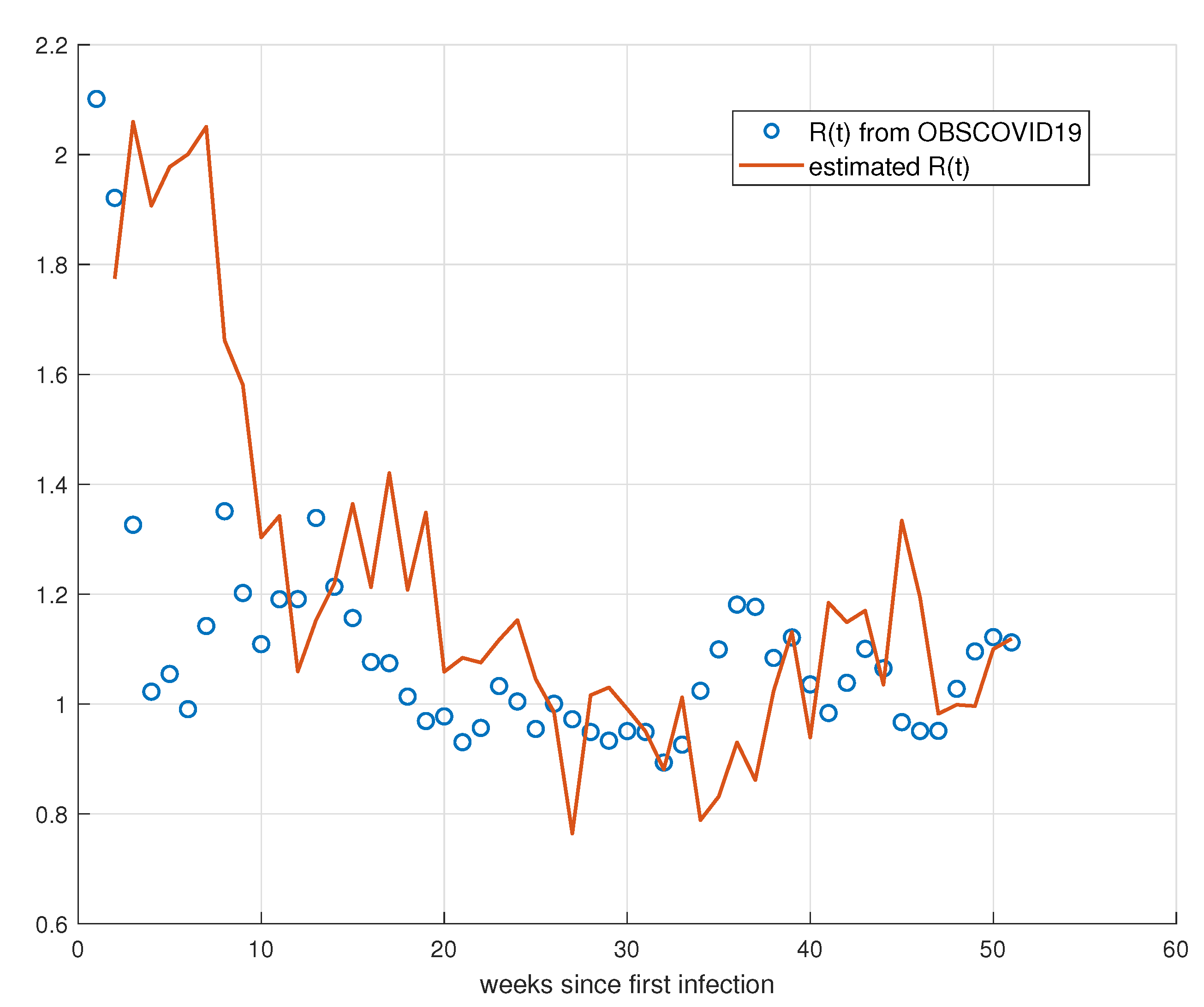
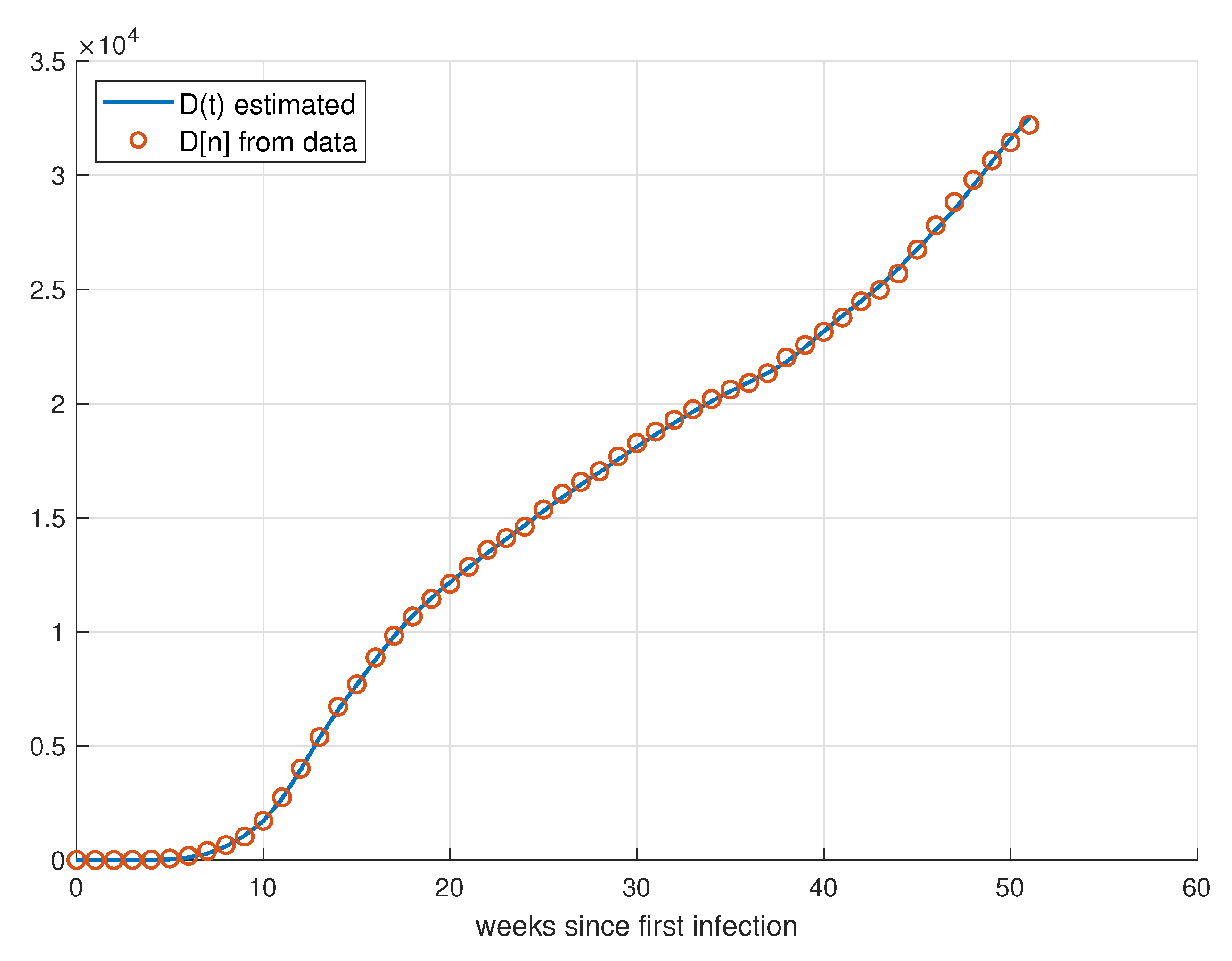
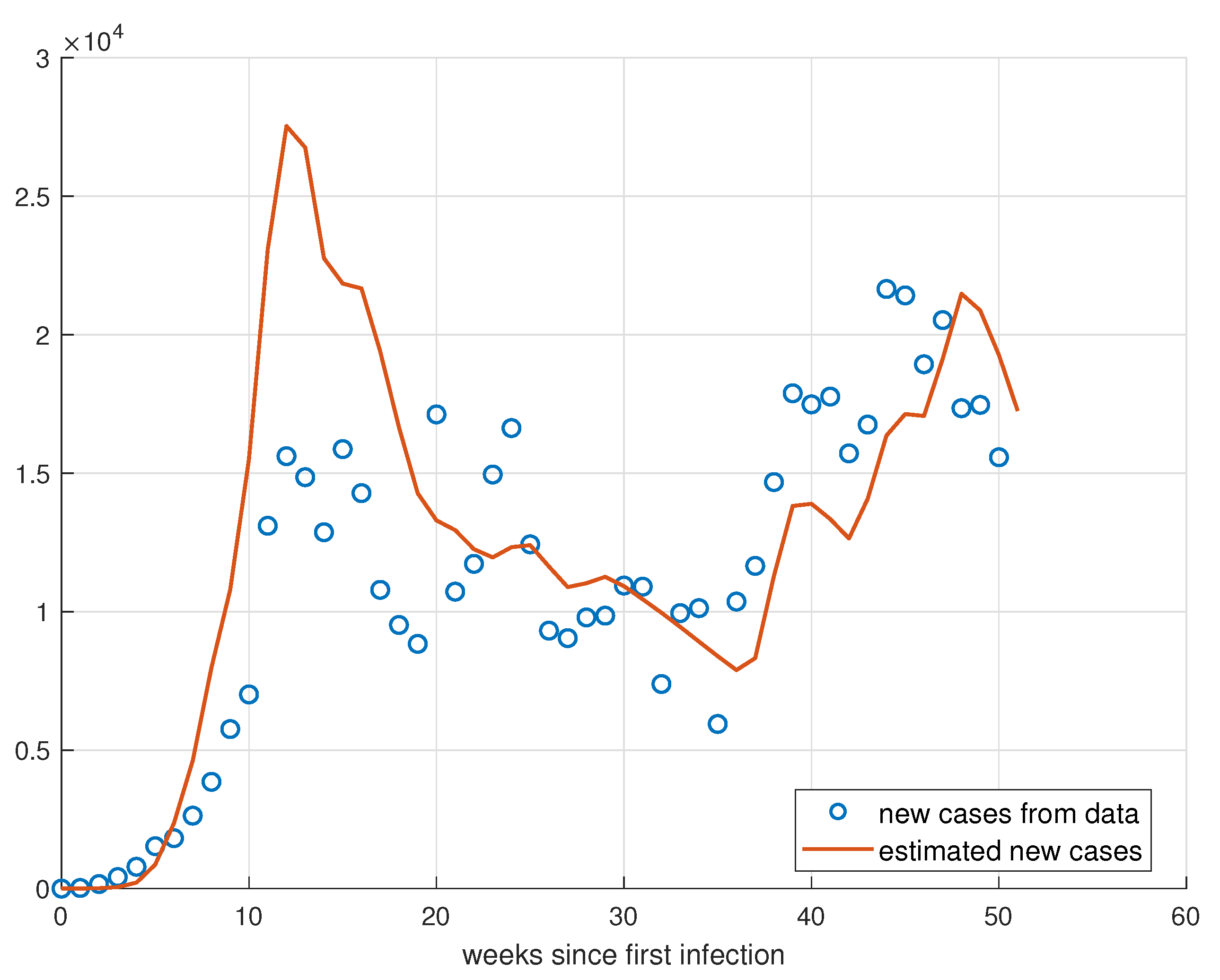
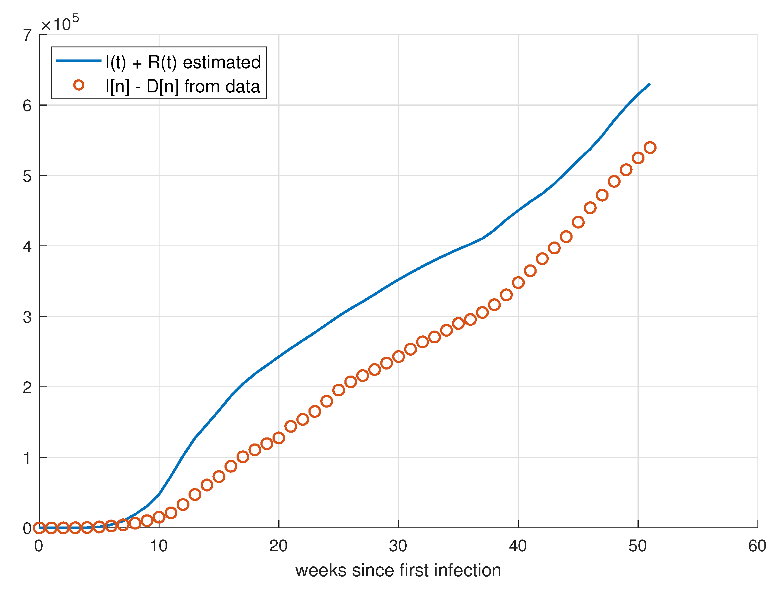
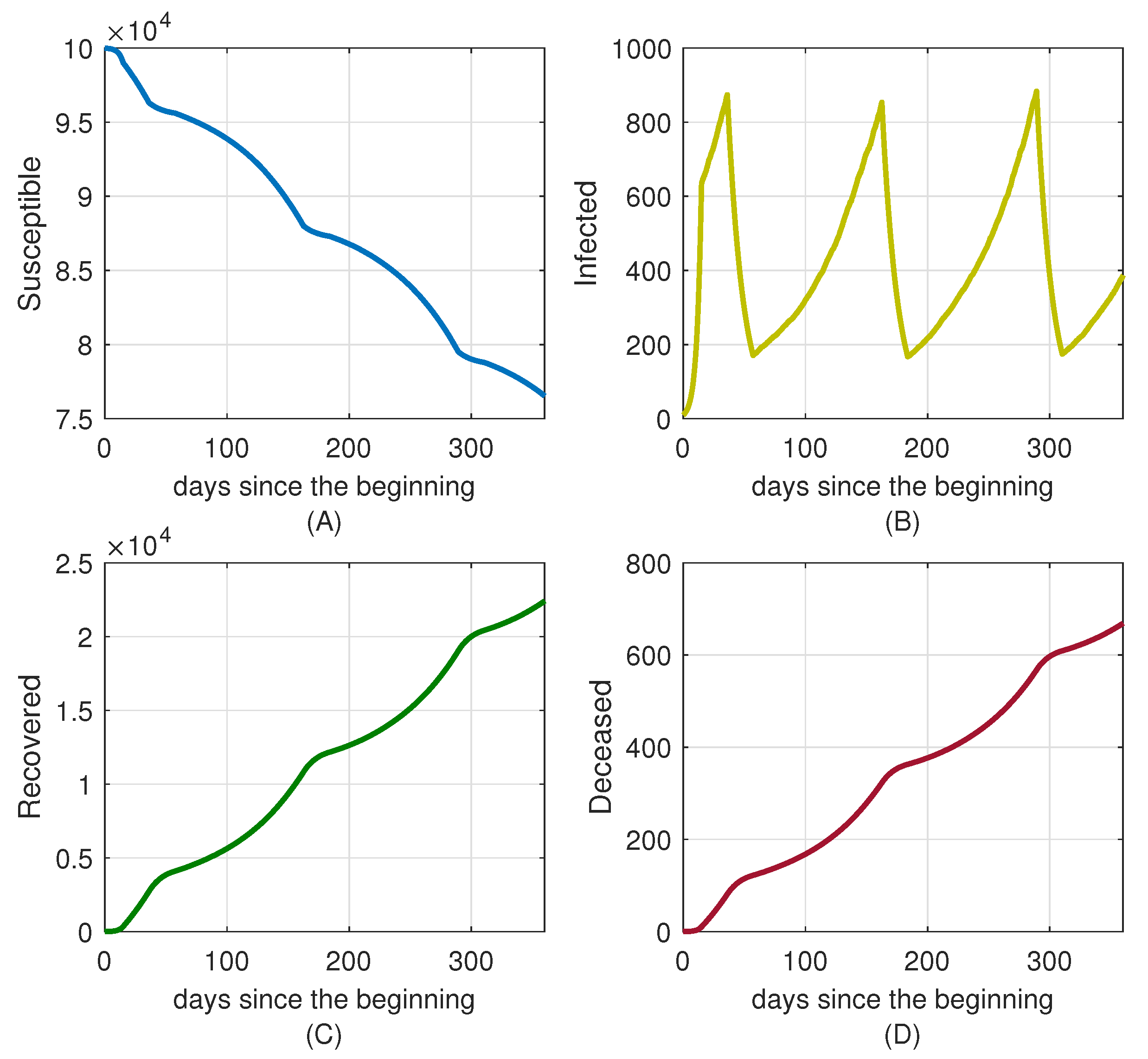
5. Validation for the SIRD Model

In this study, we used one year of epidemiological data from the states of São Paulo, Minas Gerais and Rio de Janeiro, starting on each state’s first day of infection, to validate the SIRD model.
First, the fitting process using the parameters that generate the curve that best fits the data from the model was made using daily data. However, for this large volume of data, the minimization algorithm produced a lot of noise, or overfitting, in addition to having weekly seasonality due to irregular notification dynamics. Thus, the use of weekly data was considered more suitable.
The procedure was performed to try to minimize the functional given by Equation (17). The adopted SIRD model assumes that the parameters γ and Ω are invariant in time, while the parameter β is variable in time. So, for 52 weeks, there are 54 parameters to be estimated. The process was carried out in successive steps and, instead of performing only one minimization for the 52 weeks, minimization was performed every 15 weeks, with each step accumulating the values obtained for the previous set of weeks and calculating the values of β only for the following weeks while adjusting the values of γ and Ω . Furthermore, a regularization term was inserted in the Tiknovov regularization structure, penalizing sudden variations to produce a smoother curve.
m i n θ = τ 1     ( I t c u m D t ) ( I ^ t R ^ t )     2 + τ 2     D t D ^ t     2 + τ 3       Γ B     2 .
The first term of the functional θ represents the total number of infected people since the beginning of the count, while the second term represents the total number of deaths that occurred due to the disease. Finally, the last term represents a regularization which penalizes the differences between the successive terms of β , represented by the matrix B (19), whose differences are calculated by the matrix Γ  (18):
Γ = 1 1 0 0 0 1 1 0 0 1 1
B = [ β t = 0 β t = 1 β t = T ] T .
In this way, better results could be obtained, as can be seen in the validations made for the states of São Paulo, Rio de Janeiro and Minas Gerais. In them, the value of R e was calculated as described by Equation (20):
R e ( t ) = β ( t ) γ + Ω S ( t ) N ( t ) .
The effective reproduction number is the average number of infected individuals per infected person under existing conditions at a given time. The effective number, R e , is the basal reproduction number, R 0 exposed to the real conditions of disease evolution. Consequently, it constantly changes, reflecting interaction between the population and the infectious agent [67,68].
The effective reproduction number R e was estimated by finding the values that minimize the function described by Equation (18). For Equation (21), β ( t ) is considered variable over time, because, due to restriction measures imposed by public policies, the transmission or contagion rate is altered, and, consequently, the key number S ( t ) also varies according to this rate. Although N ( t ) represents the total population and it is variable over time, for the considered interval, this constant value can be adopted.

5.1. Validation for São Paulo

For the state of São Paulo, the time-invariant parameters obtained and used can be seen in Table 2.
Where a value of 1.0701 for γ means that the average recovery period is 1.0701 weeks, and a value of 2.85% for Ω means 2.85% of infected people are killed by the virus per week.
As can be seen in Figure 11 and Figure 12, the fit for the values of the new weekly deaths and new accumulated deaths performed well, as these were privileged through the manipulation of parameters τ 1 , τ 2 and τ 3 . We see that the fit for the value of new cases in Figure 13 and Figure 14 was not as accurate as the previous fit, practically maintaining qualitative behavior.
For the graph of the effective reproduction number R e  Figure 15, it can be noted that the values were close to those obtained by the COVID-19 observatory [69], which is an independent initiative resulting from the collaboration between researchers who performed this measurement using their own methodology. There is a large divergence around 35 weeks. For the model developed in this report, the value obtained from R e makes sense, since there was a very sharp decrease in new cases and deaths in this period.

5.2. Validation for Minas Gerais

The time-invariant parameters for the state of Minas Gerais can be seen in the Table 3:
Here, it can be noted that the values of γ and Ω were quite close to the values obtained for São Paulo. Observing the graphs of new weekly deaths in Figure 16 and accumulated deaths in Figure 17, it can be seen that the model fit for these data had good performance, as well as for São Paulo.
For the data of new cases in Figure 18 and accumulated cases in Figure 19, the model performed very well until around the 35th week, when it started to present a slight difference, maintaining qualitative behavior.
For the data of R e , it is possible to notice that there is possibly a delayed relationship between the values obtained by the model and the values obtained by the COVID-19 observatory [69], as can be seen in Figure 20.

5.3. Validation for Rio de Janeiro

For the state of Rio de Janeiro, the time-invariant parameters can be seen in Table 4.
For the state of Rio de Janeiro, the value of Ω appears to be higher than for the other two states, while γ was close to the values found for São Paulo and Minas Gerais.
The analysis of Figure 21 and Figure 22 shows that the fit of the model for the data of new weekly deaths and deaths accumulated in weekly reports performed well.
For the state of Rio de Janeiro, the fit for the data of new weekly cases and accumulated deaths is similar to the São Paulo fit, indicating a possible under-reporting of cases throughout the period, as shown in Figure 23 and Figure 24.
As for both other states, the effective reproduction number appears to have some delay with respect to the number obtained by the COVID-19 observatory [69], as shown in Figure 25.

6. Spread Control

Applications of control theory for epidemic diseases, including COVID-19, range from optimal control, which can be used for social distancing [70], vaccine deployment policy [71] or even a mix of isolation and a vaccination program [72], to model predictive control (MPC), which is also used for the development of social distancing [73,74] and vaccination policies [75]. However, the approach to be followed here is simpler and aims to build an algorithm explicitly programmed through feedback of state variables, similar to other heuristics [76,77] already studied.
Practical usage of the control algorithm proposed should consider the availability and uncertainty of current infection data, which are usually embedded with under-reporting and significant delays when compared with reality, especially in countries which do not have a thorough testing program organized. It should review the simplifications assumed in the model formulation in Section 2 as well, addressing the peculiarities of the disease being analyzed.
Looking forward to the future, the algorithm should address any disease that follows the same pattern of transmission of the coronavirus, that is, infections resulting from the transportation of contaminated droplets of secretions from infected individuals to susceptible ones and that suggests isolation is effective. The main difference will be the difficulty imposed by a new virus concerning the imposition of lower values of R e , a parameter which is described in the next section. Viruses that are transmitted more easily impose a bigger challenge, as fewer contacts are needed to effectively pass the disease ahead.

Algorithm Implementation

Here, the implementation of a three-level stratified controller is studied, mitigating disease spread, aiming to maintain the demand of intensive care units (ICUs) lower than those available at all times until a vaccine is available.
As was shown, R 0 measures how the disease propagates when there are almost no infected individuals present ( S N ). While R 0 provides valuable information on the viral dissemination dynamics when there is no developed immunity and information on the epidemic available, other factors begin to influence its dynamics during the course of spreading.
Therefore, the effective reproduction number R e , which describes the average value of secondary infections as a time-dependent function, is a more appropriate parameter to be analyzed amidst an epidemic outbreak [78]. In a homogeneous population, it is simple to obtain R e by multiplying R 0 and the susceptible proportion of the population at some instant t [79].
The idea to be developed here is to regulate R e in order to maintain the healthcare resources at an acceptable level. The underlying mechanism is the manipulation of the contact rate of individuals β by cycling the imposition and relaxation of social distancing measures [57] as well as awareness campaigns to stimulate the adoption of individual protection procedures.
Therefore, β is no longer considered fixed but time-dependent β ( t ) . Contrarily, γ and Ω are still considered invariable, as treatments such as the use of remdesivir or monoclonal antibodies, both approved by the American Federal Drug Administration (FDA), are prescribed only to severe cases whereupon the patient is already hospitalized and therefore isolated [80,81] in the first case, while, in the latter, it took almost a year to be approved for emergency use [82].
Levels of the controller are decided based on the current number of patients needing an ICU. This number is defined as 5% of the current number of infected individuals, assumed as the probability of someone who becomes infected needing intensive care [83].
Each level is composed of an interval from which R e can randomly assume any value. The interval is constructed with limits equal to ±10% of the measured mean value. This is performed to mimic the difficulty of imposing and tracking a precise value for R e for diseases with only a few epidemic studies.
The stratified controller model was chosen due to being easier to implement than other forms of modeling social distancing, generally based on continuous values for R e , which are very hard to track and impose precisely. The algorithm is also adaptable structurally speaking, as the R e should necessarily guarantee the desired behavior according to the model. The most significant difficulties rest in creating the appropriate public policies to reach the desired R e level.
Estimations of the economic impact of the COVID-19 pandemic are situated close to the trillion dollars figure globally [84,85,86], with devastating shocks on various industries, and the imposition of social distancing policies should have been, theoretically, a big part of this loss. However, there is significant evidence that quarantine is effective against not implementing containment mechanisms [87], more effective when applied early [88] and that deterioration of economic conditions preceded the introduction of isolation policies [89] or that the culprit of the COVID-19 recession is COVID-19 itself [90]. Therefore, practical usage of the three-level controller should lead to economic benefits, not to mention that saving lives should be worth the cost nevertheless.
The three-level controller is described in Table 5, with the calibration level (mitigation or suppression) related to the value of the reproduction number associated. Mitigation and suppression measures differ in whether they aim to reduce the reproduction number, R e , to less than 1 (suppression) or to merely slow spread by reducing R e but not to less than 1 (mitigation) [91]. Therefore, Level A can be described as mitigation strategy and Level C as a suppression one, generally called a lockdown, while Level B is situated between both.
All the actions taken at a certain point will last for a regularly chosen duration during the course of the pandemic. This is performed to reduce social and economic uncertainty as the population has time to comply.

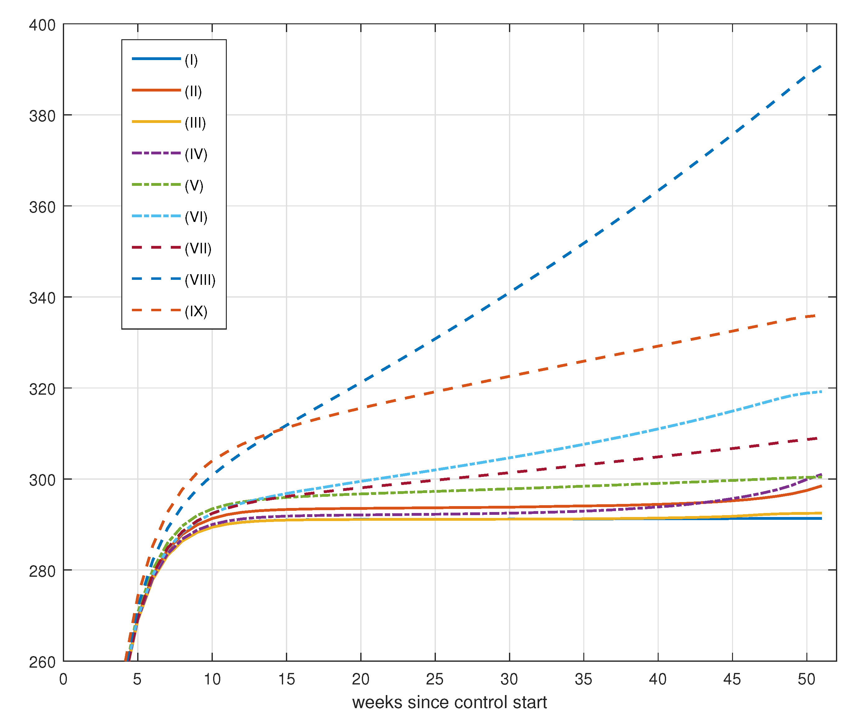
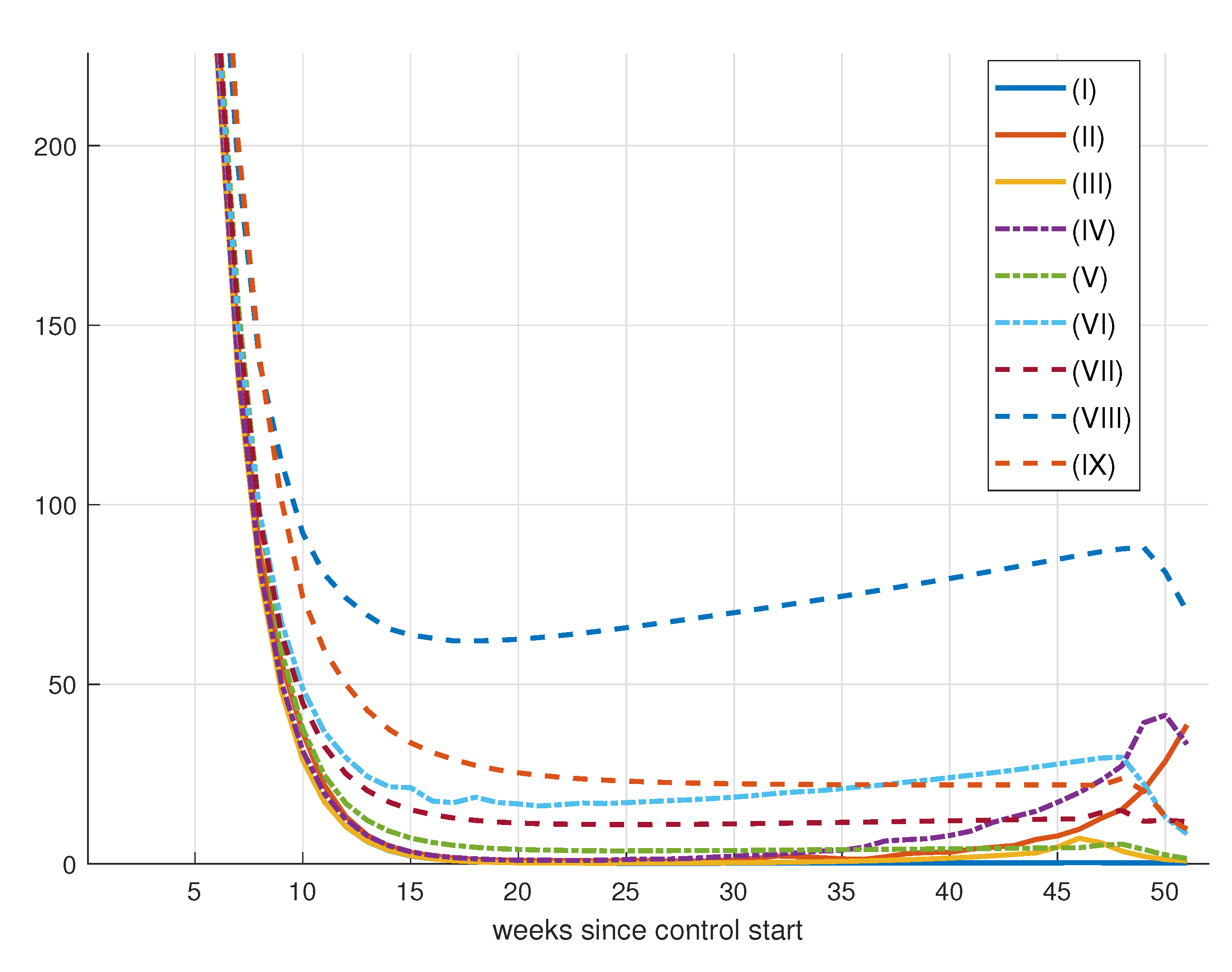
7. Control Strategy Results

In this section, the three-level control strategy described in the former section is simulated assuming a hypothetical scenario for an isolated city in Brazil with 10 infected initial cases, a population of 100,000 inhabitants and an R 0 the same as the country’s, i.e., 2.82. This number is maintained for the first 15 days to replicate initial unawareness. Brazil was chosen due to its high baseline contact rate, represented by the high value of R 0 , as opposed to Uruguay. Therefore, as the number of cases and individuals in need of ICUs grow faster than the system can adapt, it represents a need for establishing isolation policies.
The number of ICUs available is considered to be 50, very close to the proportion of beds/individuals obtained for the state of São Paulo before the pandemic in 2018 [95].
The total period analyzed is one year, because this is the period assumed for the development of a vaccine, with reference to the Pfizer vaccine, which started being developed in January 2020 with the release of the SARS-CoV-2 genome [96] and initially applied in the UK at the beginning of December 2020 [97].
Three different strategies were considered: no attempt to control the disease spread; updating R e every 30 days; and updating R e every 21 days.

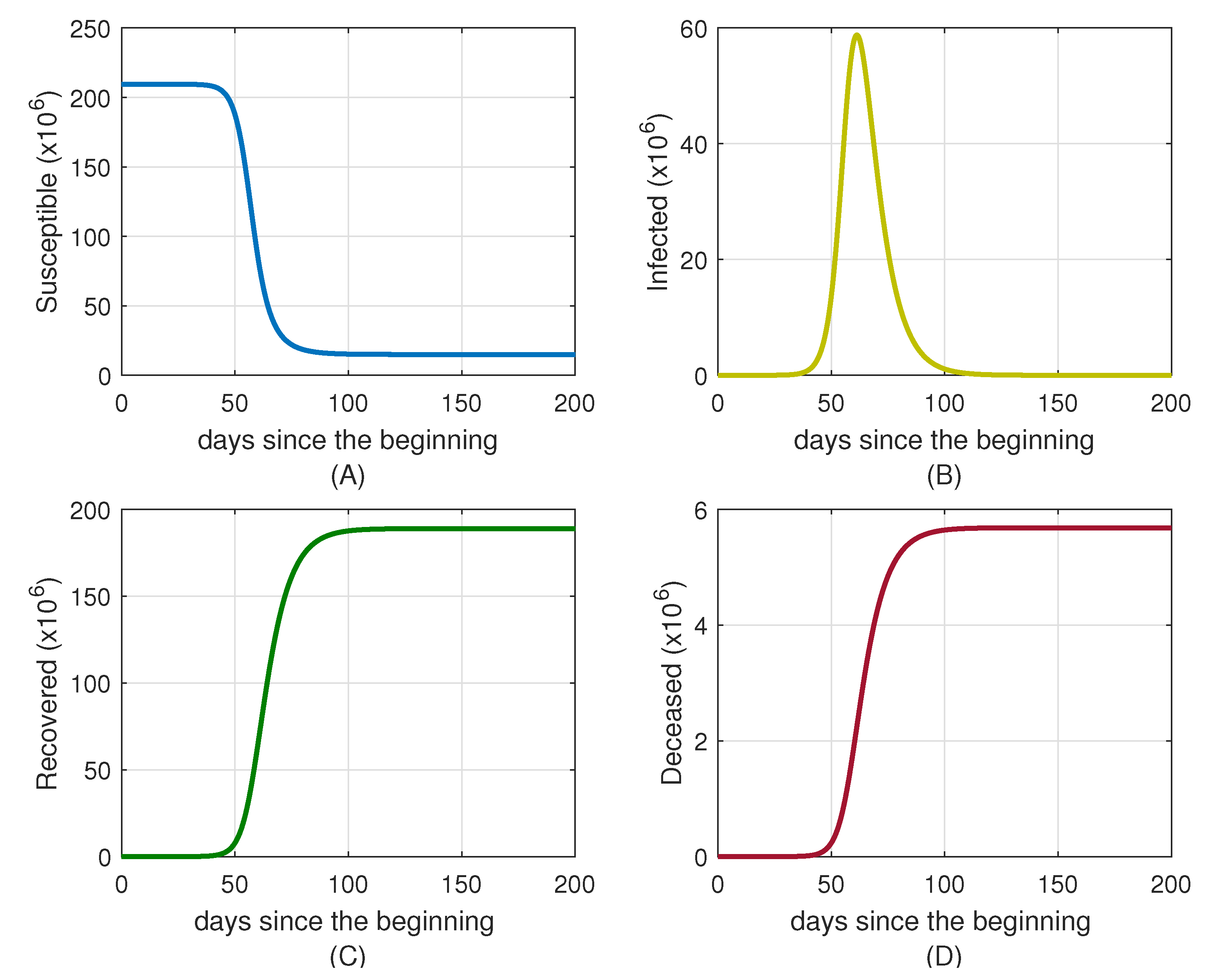
7.1. No Attempt to Control the Spread of the Disease

As expected, Figure 26 shows the potential of COVID-19 to quickly overwhelm the healthcare system, with ICU demand surpassing the availability of beds less than two months after the beginning of the pandemic. The randomness added did not result in significant differences with respect to the baseline established in Section 4.
The dynamics of free dissemination can be seen for all the compartments in the SIRD model used in Figure 27.

7.2. Updating R e Every 30 Days

Figure 28 displays the algorithm’s performance for a 30-day interval between updates regarding the demand for ICU and shows the controlled reproductive number R e for each cycle. It can be seen that after periods of Level C (lock-down), ICU demand went below 10% of the total number of intensive care beds available, which made the algorithm choose Level A for the following cycle.
Every time this happened, the control failed to prevent healthcare collapse, as 30 days proved to be enough time for Level A to allow a large increase in demand for ICU due to the exponential growth nature of the spread.
The improvement over the baseline was very small, as can be seen in Figure 27D, with the number of deceased at the end of the period being very close to the number of deceased at the end of the baseline.
Figure 29 supports the effectiveness of the algorithm wiyh a 30-day cycle. Therefore, in order to prevent the ICU demand from surpassing the supply of intensive care beds, the period between updates of the algorithm is reduced, and results are shown in Section 7.3.

7.3. Updating R e Every 21 Days

For a 21-day interval between updates, the main goal of guaranteeing appropriate care for COVID-19 patients is attained. During the 360 days of simulation, there was no instant at which the demand for intensive care units was greater than the supply, as shown in Figure 30, and there were only three periods of Level C (lock-down), allowing individuals to have greater freedom without sacrificing effectiveness.
Figure 31 supports the effectiveness of the algorithm with a 21-day cycle, showing much fewer deaths at the end of the simulation than in simulations I (baseline) and II (30-day cycle).

8. Epidemic Control

In this section, two ways of controlling the spread of the coronavirus pandemic are studied. First, a social distancing policy is applied, followed by a vaccination campaign.

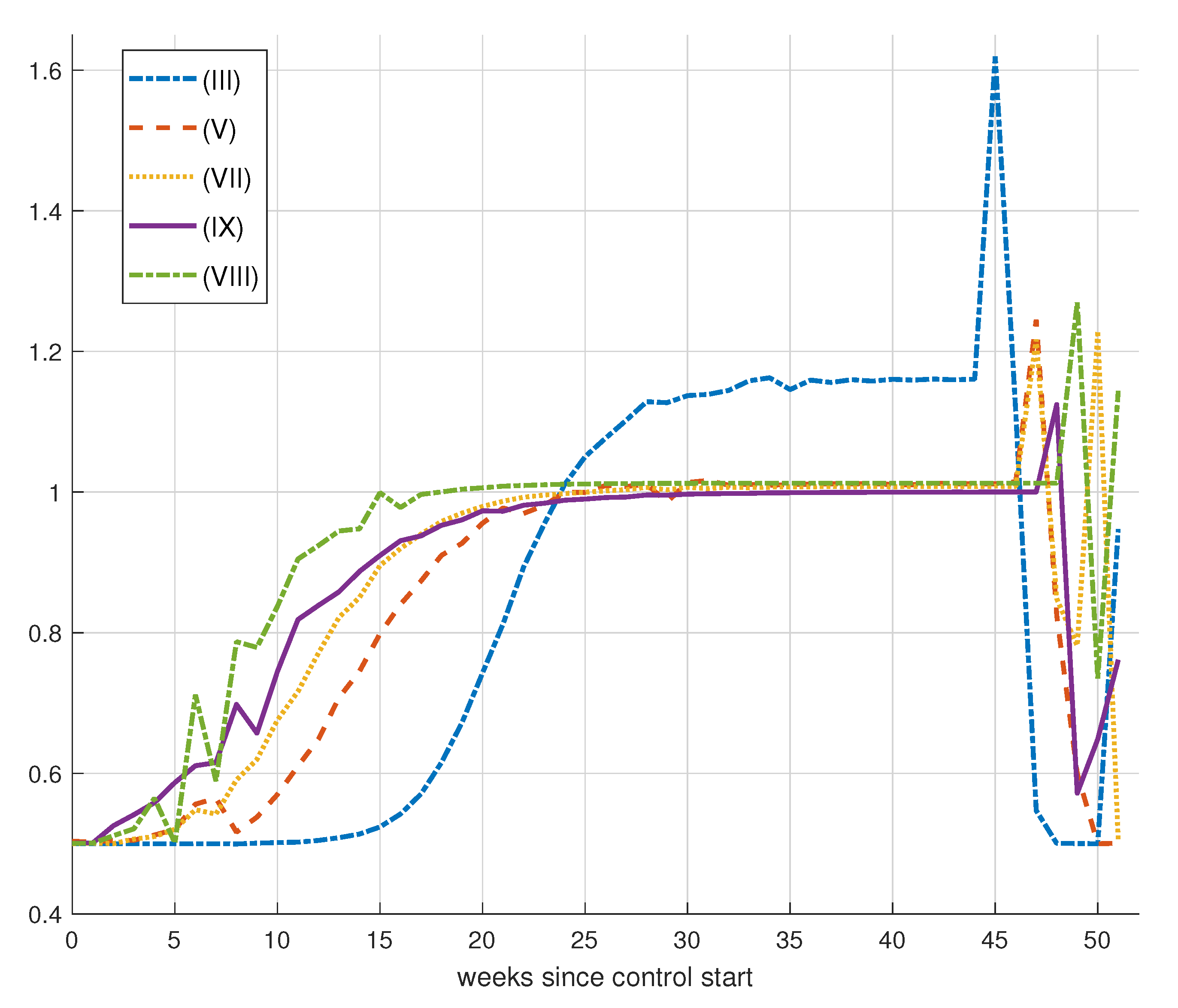
8.1. Control by Social Distancing

The simulation of control by social distancing was carried out in the context described in Table 6.
The values of γ and Ω adopted were based on the values obtained in the validation for São Paulo and Minas Gerais. We simulated 52 weeks, which is the amount of time it takes to develop a vaccine for the virus, with reference to the Pfizer vaccine, whose development started in January 2020 and was released in December 2020.
The initial number of infected is reasonably high to simulate a situation in which there is little information about the spread of the virus in the population studied. Additionally, a minimum value for the effective reproduction number is implemented, reflecting the highest capacity possible for public authorities to implement isolation measures in the population. This value is 0.5 and is close to the value obtained for Spain in its lockdown in 2020 [94].
The application of social distancing control was carried out by manipulating the parameter β ( t ) so that the value of the effective reproduction number R e was sufficiently low to bring about a reduction in the number of new cases and weekly deaths.
The applied control was found from the formulation of a minimization problem to find a sequence of controls represented by (22):
u [ k ] = [ u ( 0 ) u ( 1 ) u ( 2 ) u ( K 1 ) ] ,
with the objective of minimizing the functional J (22):
J = τ 1 D ( t = T f ) τ 2     u [ k ]   2 + τ 3       u [ k ] u [ k 1 ]   2 .
The first term of Equation (22) represents the number of accumulated deaths at the end of the period (in t = T f ) ; the second term, u [ k ] = β [ k ] , represents the control applied at instant k; and the last term represents the control differential between instant k and k 1 . The intention behind the first term is self-explanatory: the aim is to minimize the total number of deaths at the end of the period. In contrast, a very low level of isolation has severe social and economic consequences, which is why the second term is used, which penalizes a very intense control. Finally, it is desirable that the control signal, social distancing, does not vary much from week to week to reduce future uncertainties for the population.
In addition, the restriction was imposed that at no time did the number of people in need of medical treatment exceed the number of available hospital beds, as proposed in Equation (23):
0.2 I ( t ) L , t
The definition of 20% as the percentage of infected people who need hospital treatment was obtained by observing the figure and information available at the São Paulo State Health Department (https://www.saopaulo.sp.gov.br/planosp/simi/leitos/) (acessed on 20 June 2020).

Results for Social Distancing Control

As this is an optimization problem, an important factor is the choice of parameters τ 1 , τ 2 and τ 3 that will drive the functional J. Variations in these parameters are related to the prioritization or penalty that gives the terms referring to the number of deaths, minimization of social distance and distance differential. Therefore, five different combinations were studied for the set ( τ 1 , τ 2 , τ 3 ) , with the results summarized in Table 7 and in Figure 32.
It can be noted that an increase in τ 2 , which is a greater prioritization of maximizing the norm of β , resulted in an increase in the number of deaths at the end of the period. Meanwhile, increases in τ 3 generally had the effect of reducing the norm of the applied controls differential, as was desired, and a reduction in the variability of R e can be seen in the graphs below. At the same time, it produced a reduction in the number of deaths, which was unexpected.
By analyzing the graph, it is possible to notice the increase in the number of deaths accumulated in time when the value of τ 2 is increased. The effective reproduction number graphs were divided into two parts, because those in Figure 32 were very noisy, making visualization difficult. This more intense noise occurred precisely in the graphs that were associated with an increase in τ 2 without an increase in τ 3 associated.
The qualitative analysis of Figure 33 and Figure 34 shows that there is a very intense control in the first weeks, in order to quickly reduce the number of cases to zero, as shown in Figure 35. After this period, there is a gradual release of distancing, implying a gradual increase in R e , followed by a new constraint near the end of the period.
A more detailed study considering social distancing as a strategy to control the spread of COVID-19 was performed in [50]. The proposed model, which consists of an alteration of the SIR model, considers the infected in two compartments: the infected being reported and the infected not reported or asymptomatic. The validation of the model is carried out for different cities in the state of São Paulo and allows the evaluation of the dynamics of disease reinfection and the relevance of social distancing as cities adhere to social isolation at different times.

8.2. Vaccination Control

To implement the vaccination control, a new term v ( t ) was introduced in the equations that describe the system, now formulated by the set of Equation (24).
d S ( t ) d t = β S ( t ) I ( t ) N v ( t ) d I ( t ) d t = β S ( t ) I ( t ) N ( γ + Ω ) I ( t ) d R ( t ) d t = γ I ( t ) + v ( t )
The term v ( t ) represents the number of individuals vaccinated at time t, and all parameters, β , γ and Ω , are considered constant, representing a situation in which there is no change in the behavior of the population regarding the contact rate between individuals, that is, there is no social distancing. Again, the solution to this problem is given by minimizing a functional, described by Equation (25), where we want to minimize the number of deaths while also minimizing the cost of vaccination.
J v a c = τ 1 D ( t = T f ) + τ 2     v [ k ]   2 + τ 3       v [ k ] v [ k 1 ]   2
In addition, it is desirable to minimize the vaccine immunization differential, represented by the last term of the functional, so that there is not a very sudden variation in the number of vaccines given from one week to the next.

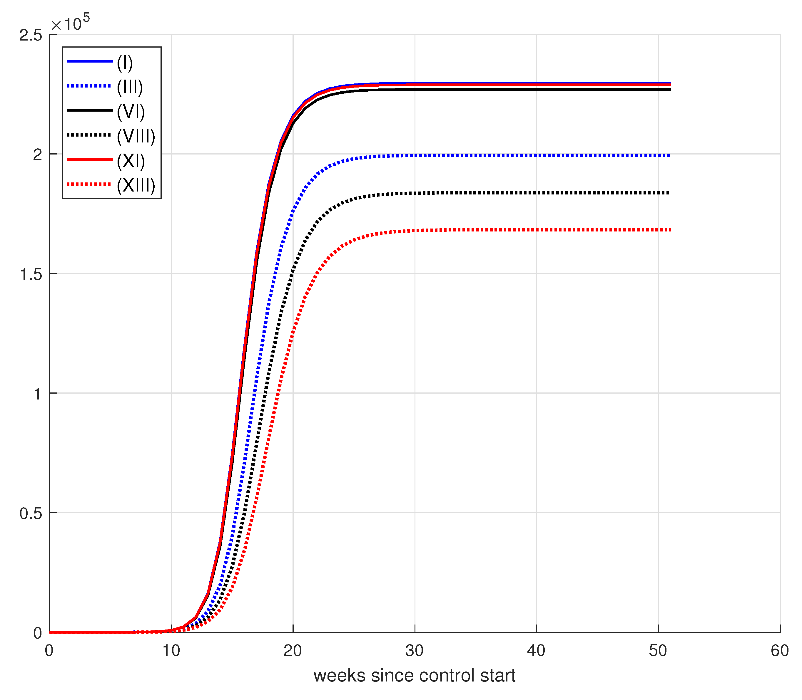
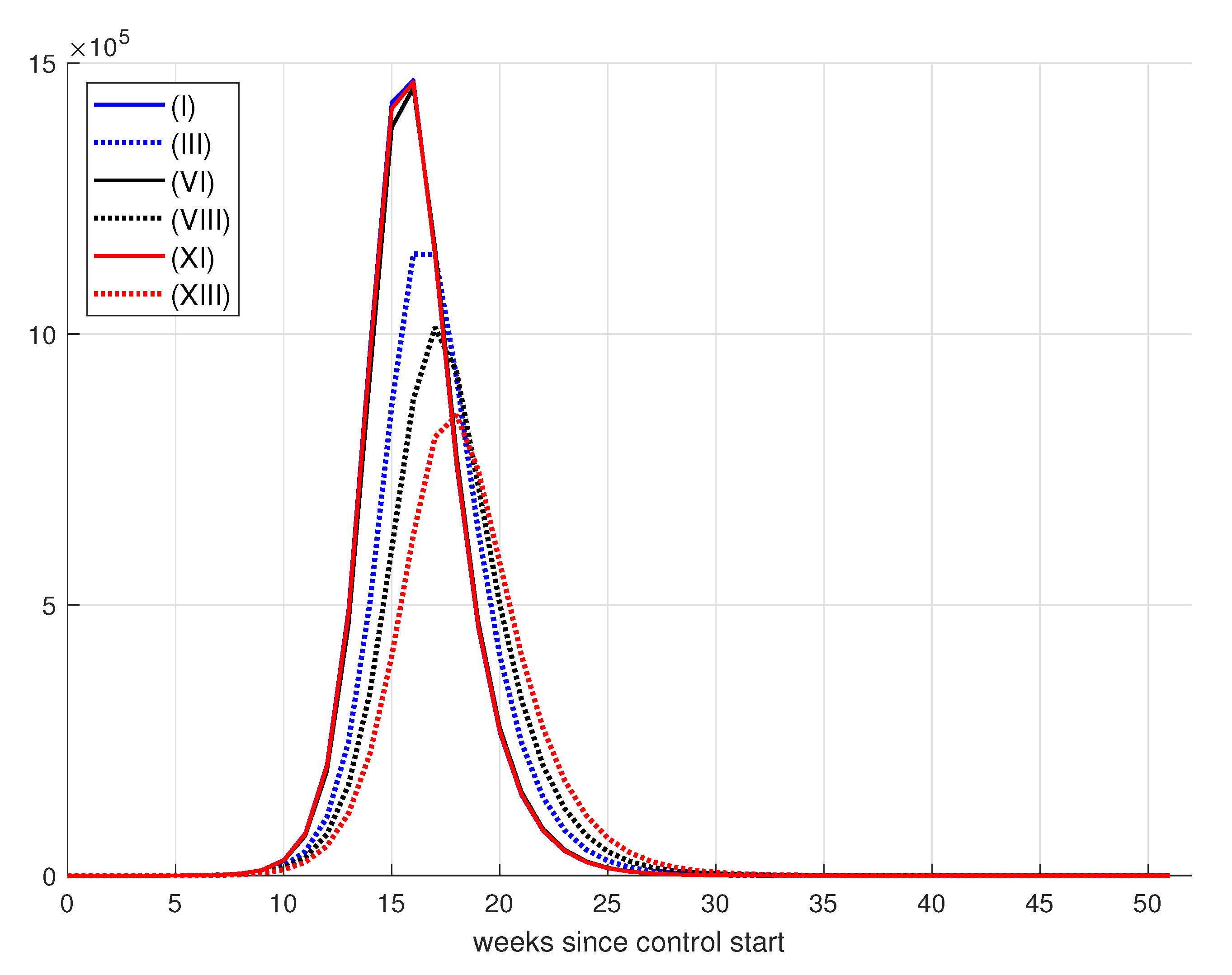
8.2.1. Results for Vaccination Control

The simulation parameters for vaccination control can be seen in Table 8:
Regarding the simulation for vaccination control, the number of initial infected people was reduced to simulate a condition that is still at the beginning of the spread of the disease. Also, there is no longer a minimum value for the effective reproduction number, since the value of the contact rate between individuals β is considered fixed. The value of β is fixed at 2 ( γ + Ω ) , representing a base reproduction number value R 0 equal to 2.
A maximum value of vaccinated per time instant is established to represent scenarios in which there are limited availability of vaccines to be applied. The results obtained are compiled in Table 9.

8.2.2. Effect of Increase in Weekly Vaccination

The first part of the simulations analyze the effect of increasing the limit of application of vaccines weekly. As expected, Figure 36 shows that increases in the weekly vaccination limit, when associated with an increase in the weight τ 1 , which refers to the number of deaths at the end of the period, reflect a significant drop in this value.
The analysis of the weekly new cases graph reflects the same behavior. Figure 37 shows that an increase in vaccination reduces the number of new weekly cases when the weight τ 1 is increased, which prioritizes a reduction in the number of deaths in relation to the cost of administering vaccines.
Another interesting fact is that the weekly vaccination rate obtained for conditions where τ 1 is much greater than τ 2 and τ 3 is not the maximum vaccination vector at all times. It can be noted in Figure 38 that in none of the cases, the maximum vaccination for the period in 26%, 39% and 52% of the population, respectively, was reached. This is because the model assumes obtaining immunity after recovering from the disease. Therefore, individuals who were not vaccinated either died or recovered.
A severely negative point of the application of control only by vaccination is that the limit of the number of available hospital beds was not respected, as can be seen in Figure 39. In the tenth week, the health system collapses.

8.2.3. Effects of Changes in Vaccination Campaign Prioritization

To highlight the policy changes when we prioritize the number of deaths over the cost of vaccination or vice versa, Figure 40, Figure 41 and Figure 42 are presented, related to cases (VI) to (X) of the prioritization parameters. First, Figure 40 shows that the increase in τ 1 in the case (VI) pro (VII) and (VII) pro (VIII) showed a decrease in the number of accumulated deaths, as expected; likewise, from case (VIII) to (IX), in which an increase in τ 2 is considered, the graph shows an increase in the number of accumulated deaths.
Analogously to the case of control by social distancing, where there is a drop in the number of deaths, an increase in τ 3 , which penalizes the variation in the control vector v ( t ) , also showed a drop in the number of deaths.
A more detailed study considering validation with real data of the control strategy based on vaccination was carried out in [51]. The model considers the possibility of reinfection and allows checking information on unreported infected people. The validation of the model was carried out with data from the city of São Paulo, which, due to its sociodemographic and economic difference, presents complex scenarios and can be extended to regions with the same qualitative characteristics.

9. Conclusions

Inspired by the different policies of social distances adopted by Brazil and Uruguay, showing remarkable differences concerning the results of controlling the COVID-19 epidemic, a framework for modeling and applying public policies in the form of social distancing was proposed aiming for a reduction in disease spread.
Validation of the SIRD model using cumulative case data and cumulative death data for the states of São Paulo, Minas Gerais and Rio de Janeiro proved satisfactory. For the accumulated death data, the performance was good, while for the accumulated case data, the performance was average, with advances in relation to previous results. Possibly, a better relationship between deaths and cases should be explored, such as inserting delay terms into the equations, or else considering the γ and Ω parameter variables, as we conducted with β .
Comparison of data on the effective reproduction number R e obtained by the model with respect to the values obtained by a COVID-19 observatory showed a delay, possibly due to the difference in the methodology used. The work proposes a minimization of square errors for the developed model, while a COVID-19 observatory performed the estimate using serial intervals, defined as the time interval between the onset of illness in a primary case and the onset of illness in a secondary case [69].
Control by social distancing performed well, complying with the restrictions imposed. At all times, there was no failure of the health system. However, during the 52 weeks, the level of isolation remained intense without returning to the preisolation level. Also, continuous levels of R e would likely be quite difficult to implement. For example, in practice, it is difficult to implement public policies with an R e of 0.9 versus R e of 0.95.
Meanwhile, vaccination control reduced the number of accumulated deaths at the end of the period, but it did not prevent the failure of the health system. In this way, social distancing is necessary until herd immunity is reached, the value at which a primary infection produces, on average, less than a secondary infection, which eventually leads to the extinction of the disease.
The results are satisfactory, mainly due to the good performance shown for the accumulated death data, which allowed the use of the model to apply social distancing control and vaccination control.
A three-level controller was proposed, and simulations indicate that a 21-day update strategy shows good results, preventing the healthcare system from collapsing and presenting much fewer deaths at the end of the process.
Aspects to be explored to improve the model are to consider the algorithm behavior varying R e for each level, to have a different number of levels and to include uncertainty and delay in the observability of the number of infected cases.
Despite being an intuitively obvious conclusion, it was shown that failing to mitigate the spread of the disease is not a wise option. The algorithm with 21 days between updates presents, for example, almost 650 deaths at the end of the year, whereas doing nothing resulted in approximately 2700.
Therefore, it is possible to say that the framework outlined is a good and simple reference model to be followed when designing techniques to address COVID-19 disease spread, as well as possibly other diseases that follow the same pattern of transmission as the coronavirus.

Author Contributions

Conceptualization, C.B.; methodology, C.B. and J.R.C.P.; software, G.D.; validation, C.B.; formal analysis, J.R.C.P.; investigation, G.D.; data curation, G.D.; writing—original draft preparation, G.D. and C.B.; project administration, J.R.C.P.; funding acquisition, J.R.C.P.. All authors have read and agreed to the published version of the manuscript.

Funding

JRCP is supported by the São Paulo Research Foundation: 2022/00770-0 and the National Council for Scientific and Technological Development: 302883/2018-5.

Conflicts of Interest

The authors declare that there are no conflicts of interest regarding the publication of this article.

Appendix A

From Wiggins, 1990, p. 193 [98]. Consider vector fields of the form
x ˙ = A x + f ( x , y ) , y ˙ = B y + g ( x , y ) , ( x , y ) I R c × I R s ,
satisfying
f ( 0 , 0 ) = 0 , D f ( 0 , 0 ) = 0 , g ( 0 , 0 ) = 0 , D g ( 0 , 0 ) = 0 ,
where A is a c × c matrix having eigenvalues with zero real parts, B is an s × s having eigenvalues with negative real part and f and g are C r functions (r ≥ 2). Then,
Remark A1.
An invariant manifold will be called a center manifold for (A1) if it can locally be represented as
W c ( 0 ) = { ( x , y ) I R c × I R s | y = h ( x ) , | x | < δ , h ( 0 ) = 0 , D h ( 0 ) = 0 }
for δ sufficiently small.
Theorem A1.
There exists a C r center manifold for (A1). The dynamics of (A1) restricted to the center manifold is, for u sufficiently small, given by the following c-dimensional vector field
u ˙ = A u + f ( u , h ( u ) ) , u I R c .
Theorem A2.
(i) Suppose the zero solution of (A3) is stable (asymptotically stable) (unstable); then, the zero solution of (A1) is also stable (asymptotically stable) (unstable). (ii) Suppose the zero solution of (A3) is stable. Then, if ( x ( t ) , y ( t ) ) is a solution of (A1) with ( x ( 0 ) , y ( 0 ) ) sufficiently small, there is a solution u ( t ) of (A3) such that as t
x ( t ) = u ( t ) + O ( e γ t ) , y ( t ) = h ( u ( t ) ) + O ( e γ t ) ,
where γ > 0 is a constant.

References

  1. Velavan, T.P.; Meyer, C.G. The COVID-19 epidemic. Trop. Med. Int. Health 2020, 25, 278–280. [Google Scholar] [CrossRef]
  2. Wu, Z.; McGoogan, J.M. Characteristics of and important lessons from the coronavirus disease 2019 (COVID-19) outbreak in China: Summary of a report of 72 314 cases from the Chinese Center for Disease Control and Prevention. JAMA 2020, 323, 1239–1242. [Google Scholar] [CrossRef]
  3. World Health Organization. WHO Timeline-Covid-19; WHO: Geneva, Switzerland, 2020. [Google Scholar]
  4. Van Doremalen, N.; Bushmaker, T.; Morris, D.H.; Holbrook, M.G.; Gamble, A.; Williamson, B.N.; Tamin, A.; Harcourt, J.L.; Thornburg, N.J.; Gerber, S.I.; et al. Aerosol and surface stability of SARS-CoV-2 as compared with SARS-CoV-1. N. Engl. J. Med. 2020, 382, 1564–1567. [Google Scholar] [CrossRef]
  5. Bai, Y.; Yao, L.; Wei, T.; Tian, F.; Jin, D.Y.; Chen, L.; Wang, M. Presumed asymptomatic carrier transmission of COVID-19. JAMA 2020, 323, 1406–1407. [Google Scholar] [CrossRef]
  6. Sohrabi, C.; Alsafi, Z.; O’Neill, N.; Khan, M.; Kerwan, A.; Al-Jabir, A.; Iosifidis, C.; Agha, R. World Health Organization declares global emergency: A review of the 2019 novel coronavirus (COVID-19). Int. J. Surg. 2020, 76, 71–76. [Google Scholar] [CrossRef]
  7. Singh, S.; Parmar, K.S.; Kumar, J.; Makkhan, S.J.S. Development of new hybrid model of discrete wavelet decomposition and autoregressive integrated moving average (ARIMA) models in application to one month forecast the casualties cases of COVID-19. Chaos Solitons Fractals 2020, 135, 109866. [Google Scholar] [CrossRef]
  8. Prem, K.; Liu, Y.; Russell, T.W.; Kucharski, A.J.; Eggo, R.M.; Davies, N. The effect of control strategies to reduce social mixing on outcomes of the COVID-19 epidemic in Wuhan, China: A modelling study. Lancet Public Health 2020, 5, e261–e270. [Google Scholar] [CrossRef]
  9. Colbourn, T. COVID-19: Extending or relaxing distancing control measures. Lancet Public Health 2020, 5, e236–e237. [Google Scholar] [CrossRef]
  10. Mishra, B.K.; Keshri, A.K.; Rao, Y.S.; Mishra, B.K.; Mahato, B.; Ayesha, S.; Rukhaiyyar, B.P.; Saini, D.K.; Singh, A.K. COVID-19 created chaos across the globe: Three novel quarantine epidemic models. Chaos Solitons Fractals 2020, 138, 109928. [Google Scholar] [CrossRef]
  11. Rai, R.K.; Khajanchi, S.; Tiwari, P.K.; Venturini, E.; Misra, A.K. Impact of social media advertisements on the transmission dynamics of COVID-19 pandemic in India. J. Appl. Math. Comput. 2020, 68, 19–44. [Google Scholar] [CrossRef]
  12. Tiwari, P.K.; Rai, R.K.; Khajanchi, S.; Gupta, R.K.; Misra, A.K. Dynamics of coronavirus pandemic: Effects of community awareness and global information campaigns. Eur. Phys. J. Plus 2021, 136, 994. [Google Scholar] [CrossRef] [PubMed]
  13. Anderson, R.M.; May, R.M. Infectious Diseases of Humans: Dynamics and Control; Oxford University Press: New York, NY, USA, 1992. [Google Scholar]
  14. Brauer, F.; Castillo-Chavez, C. Mathematical Models in Population Biology and Epidemiology; Springer: New York, NY, USA, 2012. [Google Scholar]
  15. Hethcote, H.W. The mathematics of infectious diseases. Siam Rev. 2000, 42, 599–653. [Google Scholar] [CrossRef]
  16. Dietz, K. The first epidemic model: A historical note on PD En’ko. Aust. J. Stattistic 1998, 30, 56–65. [Google Scholar] [CrossRef]
  17. Laarabi, H.; Abta, A.; Hattaf, K. Optimal control of a delayed SIRS epidemic model with vaccination and treatment. Acta Biotheor. 2015, 63, 87–97. [Google Scholar] [CrossRef]
  18. Aldila, D.; Götz, T.; Soewono, E. An optimal control problem arising from a dengue disease transmission model. Math. Biosci. 2013, 242, 9–16. [Google Scholar] [CrossRef]
  19. Ruan, S.; Xiao, D.; Beier, J.C. On the delayed Ross-Macdonald model for malaria transmission. Bull. Math. Biololgy 2008, 70, 1098–1114. [Google Scholar] [CrossRef]
  20. Nwankwo, A.; Okuonghae, D. A mathematical model for the population dynamics of malaria with a temperature dependent control. Differ. Equations Dyn. Syst. 2019, 30, 719–748. [Google Scholar] [CrossRef]
  21. Egonmwan, A.O.; Okuonghae, D. Mathematical analysis of a tuberculosis model with imperfect vaccine. Int. J. Biomath. 2019, 12, 1950073. [Google Scholar] [CrossRef]
  22. Omame, A.; Okuonghae, D.; Umana, A.R.; Inyama, S.C. Analysis of a co-infection model for HPV-TB. Appl. Math. Model. 2020, 77, 881–901. [Google Scholar] [CrossRef]
  23. Omame, A.; Okuonghae, D.; Inyama, S.C. A Mathematical Study of a Model for HPV with Two High-Risk Strains. In Mathematical Modelling in Health, Social and Applied Sciences; Springer: Singapore, 2020; pp. 107–149. [Google Scholar]
  24. Hattaf, K.; Yousfi, N. Optimal control of a delayed HIV infection model with immune response using an efficient numerical method. Int. Sch. Res. Not. 2012, 2012, 215124. [Google Scholar] [CrossRef]
  25. Al-Khaled, K.; Yousef, M. An analytic study of the fractional order model of HIV-1 virus and CD4 + T-cells using adomian method. Int. J. Electr. Comput. Eng. 2021, 11, 1460–1468. [Google Scholar] [CrossRef]
  26. Khan, M.I.; Al-Khaled, K.; Raza, A.; Khan, S.U.; Omar, J.; Galal, A.M. Mathematical and numerical model for the malaria transmission: Euler method scheme for a malarial model. Int. J. Mod. Phys. B 2023, 37, 2350158. [Google Scholar] [CrossRef]
  27. Kermack, W.O.; McKendrick, A.G. A contribution to the mathematical theory of epidemics. Proc. R. Soc. London Ser. A 1927, 115, 700–721. [Google Scholar] [CrossRef]
  28. Kermack, W.O.; McKendrick, A.G. Contributions to the mathematical theory of epidemics. II.—The problem of endemicity. Proc. R. Soc. London Ser. A 1932, 138, 55–83. [Google Scholar] [CrossRef]
  29. Kermack, W.O.; McKendrick, A.G. Contributions to the mathematical theory of epidemics. III.—Further studies of the problem of endemicity. Proc. R. Soc. London Ser. A 1933, 141, 94–122. [Google Scholar] [CrossRef]
  30. Khajanchi, S.; Sarkar, K.; Mondal, J.; Nisar, K.S.; Abdelwahab, S.F. Mathematical modeling of the COVID-19 pandemic with intervention strategies. Results Phys. 2021, 25, 104285. [Google Scholar] [CrossRef]
  31. Cantó, B.; Coll, C.; Sánchez, E. Estimation of parameters in a structured SIR mode. Adv. Differ. Equ. 2017, 2017, 33. [Google Scholar] [CrossRef]
  32. Ng, T.W.; Turinici, G.; Danchin, A. A double epidemic model for the SARS propagation. BMC Infect. Dis. 2003, 3, 19. [Google Scholar] [CrossRef]
  33. Danca, M.F.; Kuznetsov, N. Matlab code for Lyapunov exponents of fractional-order systems. Int. J. Bifurc. Chaos 2018, 28, 1850067. [Google Scholar] [CrossRef]
  34. Godio, A.; Pace, F.; Vergnano, A. SEIR modeling of the Italian epidemic of SARS-CoV-2 using computational swarm intelligence. Int. J. Environ. Res. Public Health 2020, 17, 3535. [Google Scholar] [CrossRef]
  35. Lin, Q.; Zhao, S.; Gao, D.; Lou, Y.; Yang, S.; Musa, S.S.; Wang, M.H.; Cai, Y.; Wang, W.; Yang, L.; et al. A conceptual model for the coronavirus disease 2019 (COVID-19) outbreak in Wuhan, China with individual reaction and governmental action. Int. J. Infect. Dis. 2020, 93, 211–216. [Google Scholar] [CrossRef] [PubMed]
  36. Piqueira, J.R.C.; Araujo, V.O. A modified epidemiological model for computer viruses. Appl. Math. Comput. 2009, 213, 355–360. [Google Scholar] [CrossRef]
  37. Piqueira, J.R.C.; Batistela, C.M. Considering quarantine in the SIRA malware propagation model. Math. Probl. Eng. 2019, 2019, 6467104. [Google Scholar] [CrossRef]
  38. Khajanchi, S.; Das, D.K.; Kar, T.K. Dynamics of tuberculosis transmission with exogenous reinfections and endogenous reactivation. Phys. A Stat. Mech. Its Appl. 2018, 497, 52–71. [Google Scholar] [CrossRef]
  39. Kucharski, A.J.; Russell, T.W.; Diamond, C.; Liu, Y.; Edmunds, J.; Funk, S.; Eggo, R.M. Early dynamics of transmission and control of COVID-19: A mathematical modelling study. Lancet Infect. Dis. 2020, 20, 553–558. [Google Scholar] [CrossRef] [PubMed]
  40. Sarkar, K.; Khajanchi, S.; Nieto, J.J. Modeling and forecasting the COVID-19 pandemic in India. Chaos Solitons Fractals 2020, 139, 110049. [Google Scholar] [CrossRef]
  41. Khajanchi, S.; Sarkar, S.; Banerjee, S. Modeling the dynamics of COVID-19 pandemic with implementation of intervention strategies. Eur. Phys. J. Plus 2022, 137, 129. [Google Scholar] [CrossRef]
  42. Giordano, G.; Blanchini, F.; Bruno, R.; Colaneri, P.; Di Filippo, A.; Di Matteo, A.; Colaneri, M. Modelling the COVID-19 epidemic and implementation of population-wide interventions in Italy. Nat. Med. 2020, 26, 855–860. [Google Scholar] [CrossRef]
  43. Rai, R.K.; Tiwari, P.K.; Khajanchi, S. Modeling the influence of vaccination coverage on the dynamics of COVID-19 pandemic with the effect of environmental contamination. Math. Methods Appl. Sci. 2023, 46, 12425–12453. [Google Scholar] [CrossRef]
  44. Mizumoto, K.; Chowell, G. Transmission potential of the novel coronavirus (COVID-19) onboard the diamond Princess Cruises Ship. Infect. Dis. Model. 2020, 5, 264–270. [Google Scholar] [CrossRef]
  45. Atangana, A. Modelling the spread of COVID-19 with new fractal-fractional operators: Can the lockdown save mankind before vaccination? Chaos Solitons Fractals 2020, 136, 109860. [Google Scholar] [CrossRef]
  46. Hellewell, J.; Abbott, S.; Gimma, A.; Bosse, N.I.; Jarvis, C.I.; Russell, T.W.; Munday, J.D.; Kucharski, A.J.; Edmunds, W.J. Feasibility of controlling COVID-19 outbreaks by isolation of cases and contacts. Lancet Glob. Health 2020, 8, e488–e496. [Google Scholar] [CrossRef]
  47. Ivorra, B.; Ferrández, M.R.; Vela-Pérez, M.; Ramos, A.M. Mathematical modeling of the spread of the coronavirus disease 2019 (COVID-19) taking into account the undetected infections. The case of China. Commun. Nonlinear Sci. Numer. Simul. 2020, 88, 105303. [Google Scholar] [CrossRef]
  48. Higazy, M. Novel fractional order SIDARTHE mathematical model of COVID-19 pandemic. Chaos Solitons Fractals 2020, 138, 110007. [Google Scholar] [CrossRef]
  49. Samui, P.; Mondal, J.; Khajanchi, S. A mathematical model for COVID-19 transmission dynamics with a case study of India. Chaos Solitons Fractals 2020, 140, 110173. [Google Scholar] [CrossRef]
  50. Batistela, C.M.; Correa, D.P.; Bueno, A.M.; Piqueira, J.R.C. SIRSi compartmental model for COVID-19 pandemic with immunity loss. Chaos Solitons Fractals 2021, 142, 110388. [Google Scholar] [CrossRef]
  51. Batistela, C.M.; Correa, D.P.; Bueno, A.M.; Piqueira, J.R.C. SIRSi-vaccine dynamical model for the Covid-19 pandemic. ISA Trans. 2023, 139, 391–405. [Google Scholar] [CrossRef]
  52. Malki, Z.; Atlam, E.S.; Ewis, A.; Dagnew, G.; Ghoneim, O.A.; Mohamed, A.A.; Abdel-Daim, M.M.; Gad, I. The COVID-19 pandemic: Prediction study based on machine learning models. Environ. Sci. Pollut. Reserach 2021, 28, 40496–40506. [Google Scholar] [CrossRef]
  53. Wieczorek, M.; Siłka, J.; Połap, D.; Woźniak, M.; Damaševičius, R. Real-time neural network based predictor for cov19 virus spread. PLoS ONE 2020, 15, e0243189. [Google Scholar] [CrossRef]
  54. Braga, M.B.; Fernandes, R.D.S.; Souza, G.N., Jr.; Rocha, J.E.C.D.; Dolácio, C.J.F.; Tavares, I.D.S., Jr.; Pinheiro, R.R.; Noronha, F.N.; Rodrigues, L.L.S.; Ramos, R.T.J.; et al. Artificial neural networks for short-term forecasting of cases, deaths, and hospital beds occupancy in the COVID-19 pandemic at the Brazilian Amazon. PLoS ONE 2021, 16, e0248161. [Google Scholar] [CrossRef]
  55. Iwendi, C.; Mahboob, K.; Khalid, Z.; Javed, A.R.; Rizwan, M.; Ghosh, U. Classification of COVID-19 individuals using adaptive neuro-fuzzy inference system. Multimed. Syst. 2021, 28, 1223–1237. [Google Scholar] [CrossRef]
  56. Iwendi, C.; Bashir, A.K.; Peshkar, A.; Sujatha, R.; Chatterjee, J.M.; Pasupuleti, S.; Mishra, R.; Pillai, S.; Jo, O. COVID-19 Patient health prediction using boosted random forest algorithm. Front. Public Health 2020, 8, 357. [Google Scholar] [CrossRef]
  57. Stewart, G.; Heusden, K.; Dumont, G.A. How control theory can help us control COVID-19. IEEE Spectr. 2020, 57, 22–29. [Google Scholar] [CrossRef]
  58. Moler, C.B. Numerical Computing with MATLAB; SIAM: Philadelphia, PA, USA, 2004. [Google Scholar]
  59. Murray, J.D. Mathematical Biology I. An Introduction; Springer: New York, NY, USA, 2002. [Google Scholar] [CrossRef]
  60. Bastos, S.B.; Cajueiro, D.O. Modeling and forecasting the early evolution of the COVID-19 pandemic in Brazil. Sci. Rep. 2020, 10, 19457. [Google Scholar] [CrossRef] [PubMed]
  61. Brauer, F.; Van den Driessche, P.; Wu, J.; Allen, L.J. Mathematical Epidemiology; Springer: Berlin/Heidelberg, Germany, 2008. [Google Scholar] [CrossRef]
  62. Guckenheimer, J.; Holmes, P. Nonlinear Oscillations, Dynamical Systems and Bifurcation of Vector Fields; Springer: New York, NY, USA, 1983. [Google Scholar] [CrossRef]
  63. Andronov, A.A.; Vitt, A.A.; Khaikin, S.E. Theory of Oscillators; Elsevier Ltd.: Pergamon, Turkey, 1966. [Google Scholar] [CrossRef]
  64. Khajanchi, S.; Bera, S.; Roy, T.K. Mathematical analysis of the global dynamics of a HTLV-I infection model, considering the role of cytotoxic T-lymphocytes. Math. Comput. Simul. 2021, 180, 354–378. [Google Scholar] [CrossRef]
  65. Dutra, C. Estimate of the basic number of reproduction R0 of COVID-19 in South American countries. Interam. J. Med. Health 2020, 3, 1–7. [Google Scholar] [CrossRef]
  66. Our World in Data. Coronavirus (COVID-19) Cases. 2021. Available online: https://ourworldindata.org/covid-cases (accessed on 7 September 2021).
  67. Bai, Y.; Peng, Z.; Wei, F.; Jin, Z.; Wang, J.; Xu, X.; Zhang, X.; Xu, J.; Ren, Z.; Lu, B.; et al. Study on the COVID-19 epidemic in mainland China between November 2022 and January 2023, with prediction of its tendency. J. Biosaf. Biosegurance 2023, 5, 39–44. [Google Scholar] [CrossRef]
  68. Wei, F.; Peng, Z.; Jin, Z.; Wang, J.; Xu, X.; Zhang, X.; Xu, J.; Ren, Z.; Bai, Y.; Wang, X.; et al. Study and prediction of the 2022 global monkeypox epidemic. J. Biosaf. Biosegurance 2022, 4, 158–162. [Google Scholar] [CrossRef]
  69. Observatório COVID-19 BR. 2021. Available online: https://covid19br.github.io/ (accessed on 28 September 2021).
  70. Kruse, T.; Strack, P. Optimal Control of an Epidemic Through Social Distancing. Cowles Found Discuss. 2020, 3581295, 2229. [Google Scholar] [CrossRef]
  71. Jaberi-Douraki, M.; Moghadas, S.M. Optimal control of vaccination dynamics during an influenza epidemic. Math. Biosci. Eng. 2014, 11, 1045–1063. [Google Scholar] [CrossRef]
  72. Hansen, E.; Day, T. Optimal control of epidemics with limited resources. J. Math. Biol. 2011, 62, 423–451. [Google Scholar] [CrossRef] [PubMed]
  73. Morato, M.M.; Bastos, S.B.; Cajueiro, D.O.; Normey-Rico, J.E. An optimal predictive control strategy for COVID-19 (SARS-CoV-2) social distancing policies in Brazil. Annu. Rev. Control 2020, 50, 417–431. [Google Scholar] [CrossRef] [PubMed]
  74. Köhler, J.; Schwenkel, L.; Koch, A.; Berberich, J.; Pauli, P.; Allgöwer, F. Robust and optimal predictive control of the COVID-19 outbreak. Annu. Rev. Control 2020, 51, 525–539. [Google Scholar] [CrossRef]
  75. Köhler, J.; Enyioha, C.; Allgöwer, F. Dynamic resource allocation to control epidemic outbreaks a model predictive control approach. In Proceedings of the 2018 Annual American Control Conference (ACC), Milwaukee, WI, USA, 27–29 June 2018; pp. 1546–1551. [Google Scholar] [CrossRef]
  76. Bin, M.; Cheung, P.Y.; Crisostomi, E.; Ferraro, P.; Lhachemi, H.; Murray-Smith, R.; Myant, C.; Parisini, T.; Shorten, R.; Stein, S.; et al. Post-lockdown abatement of COVID-19 by fast periodic switching. PLoS Comput. Biol. 2021, 17, e1008604. [Google Scholar] [CrossRef]
  77. Meidan, D.; Schulmann, N.; Cohen, R.; Haber, S.; Yaniv, E.; Sarid, R.; Barzel, B. Alternating quarantine for sustainable epidemic mitigation. Nat. Commun. 2021, 12, 220. [Google Scholar] [CrossRef] [PubMed]
  78. Khailaie, S.; Mitra, T.; Bandyopadhyay, A.; Schips, M.; Mascheroni, P.; Vanella, P.; Lange, B.; Binder, S.C.; Meyer-Hermann, M. Development of the reproduction number from coronavirus SARS-CoV-2 case data in Germany and implications for political measures. BMC Med. 2021, 19, 32. [Google Scholar] [CrossRef] [PubMed]
  79. Garnett, G.P. Role of herd immunity in determining the effect of vaccines against sexually transmitted disease. J. Infect. Dis. 2005, 191, S97–S106. [Google Scholar] [CrossRef]
  80. Centers for Disease Control and Prevention. Information for Clinicians on Investigational Therapeutics for Patients with COVID-19. 2020. Available online: https://www.cdc.gov/coronavirus/2019-ncov/hcp/therapeutic-options.html (accessed on 13 March 2021).
  81. Johns Hopkins Medicine. Is the Coronavirus Treatable? 2020. Available online: https://www.hopkinsmedicine.org/health/conditions-and-diseases/coronavirus/coronavirus-treatment-whats-in-development (accessed on 5 April 2021).
  82. FDA. Coronavirus (COVID-19) Update: FDA Authorizes Monoclonal Antibodies for Treatment of COVID-19. 2020. Available online: https://www.fda.gov/news-events/press-announcements/coronavirus-covid-19-update-fda-authorizes-monoclonal-antibodies-treatment-covid-19 (accessed on 7 September 2021).
  83. Guan, W.J.; Ni, Z.Y.; Hu, Y.; Liang, W.H.; Ou, C.Q.; He, J.X.; Liu, L.; Shan, H.; Lei, C.L.; Hui, D.S.; et al. Clinical Characteristics of Coronavirus Disease 2019 in China. N. Engl. J. Med. 2020, 382, 1708–1720. [Google Scholar] [CrossRef]
  84. COVID-19 to Slash Global Economic Output by $8.5 Trillion over Next Two Years. 2020. Available online: https://www.un.org/en/desa/covid-19-slash-global-economic-output-85-trillion-over-next-two-years (accessed on 9 September 2021).
  85. Global Economy Could Lose over $4 Trillion Due to COVID-19 Impact on Tourism. 2021. Available online: https://unctad.org/news/global-economy-could-lose-over-4-trillion-due-covid-19-impact-tourism (accessed on 9 September 2021).
  86. Global Economic Effects of COVID-19 (CRS Report No. R46270). Retrieved from Congressional Research Service Website. 2021. Available online: https://crsreports.congress.gov/ (accessed on 8 September 2021).
  87. Gupta, A.G.; Moyer, C.A.; Stern, D.T. The economic impact of quarantine: SARS in Toronto as a case study. J. Infect. 2005, 50, 386–393. [Google Scholar] [CrossRef]
  88. Demirgüç-Kunt, A.; Lokshin, M.; Torre, I. The Sooner, the Better: The Early Economic Impact of Non-Pharmaceutical Interventions During the COVID-19 Pandemic. World Bank Policy Res. Work. Pap. 2020, 26, 9257. [Google Scholar] [CrossRef]
  89. Chen, S.; Igan, D.O.; Pierri, N.; Presbitero, A.F.; Soledad, M.; Peria, M. Tracking the economic impact of COVID-19 and mitigation policies in Europe and the United States. IMF Work. Pap. 2020, 125, 25. [Google Scholar] [CrossRef]
  90. Aum, S.; Lee, S.Y.; Shin, Y. COVID-19 doesn’t need lockdowns to destroy jobs: The effect of local outbreaks in Korea. Labour Econ. 2021, 70, 101993. [Google Scholar] [CrossRef]
  91. Imperial College London. Report 9—Impact of Non-Pharmaceutical Interventions (NPIs) to Reduce COVID-19 Mortality and Healthcare Demand. 2020. Available online: https://www.imperial.ac.uk/media/imperial-college/%5Cmedicine/sph/ide/gida-fellowships/Imperial-College-COVID19-NPI-modelling-16-03-2020.pdf (accessed on 8 April 2021).
  92. Teslya, A.; Pham, T.M.; Godijk, N.G.; Kretzschmar, M.E.; Bootsma, M.C.J.; Rozhnova, G. Impact of self-imposed prevention measures and short-term government-imposed social distancing on mitigating and delaying a COVID-19 epidemic: A modelling study. PLoS Med. 2020, 17, e1003166. [Google Scholar] [CrossRef] [PubMed]
  93. G1. Governo de SP Avança 6 Regiões Para a Fase Amarela da Quarentena, Que Permite Funcionamento de Restaurantes até 22h. 2021. Available online: https://g1.globo.com/sp/sao-paulo/noticia/2021/02/05/governo-de-sp-avanca-6-regioes-para-a-fase-amarela-que-permite-funcionamento-do-comercio-ate-22h.ghtml (accessed on 28 March 2021).
  94. Hyafil, A.; Moriña, D. Analysis of the impact of lockdown on the reproduction number of the SARS-Cov-2 in Spain. Gac. Sanit. 2022, 35, 453–458. [Google Scholar] [CrossRef] [PubMed]
  95. Conselho Federal de Medicina. Medicina Intensiva no Brasil. 2018. Available online: https://portal.cfm.org.br/images/PDF/leitosdeuticapitais2018.pdf (accessed on 25 March 2021).
  96. Cleve, M.I. The lightning-fast quest for COVID vaccines and what it means for other diseases. Nature 2021, 589, 16–18. [Google Scholar] [CrossRef]
  97. CNN. UK Becomes First Country to Authorize Pfizer/BioNTech’s COVID-19 Vaccine, First Shots Roll Out Next Week. 2020. Available online: https://edition.cnn.com/2020/12/02/uk/pfizer-coronavirus-vaccine-uk-intl-hnk/index.html (accessed on 17 April 2021).
  98. Wiggins, S. Introduction to Applied Nonlinear Dynamical Systems and Chaos; Springer: New York, NY, USA, 1990. [Google Scholar]
Figure 1. SIRD model.
Mathematics 11 03766 g001
Figure 2. Simulation around the origin for τ = α ϕ .
Mathematics 11 03766 g002
Figure 3. Phase portrait for R 0 = 3   ( > 1 ) .
Mathematics 11 03766 g003
Figure 4. Phase portrait for R 0 = 0.5   < 1 .
Mathematics 11 03766 g004
Figure 5. SIRD model validation with real data from Brazil. R 0 = 2.82, γ = 0.1508, Ω = 0.0045.
Mathematics 11 03766 g005
Figure 6. SIRD model validation with real data from Uruguay. R 0 = 1.13, γ = 0.1508, Ω = 0.0045. The date 2020-04-12 presents an anomaly in the dataset, with negative new cases.
Mathematics 11 03766 g006
Figure 7. Brazilian case study with R 0 = 2.82, γ = 0.1508, Ω = 0.0045. Considering: (A) Susceptible population; (B) Infected population; (C) Recovered population and (D) Deceased population.
Mathematics 11 03766 g007
Figure 8. Phase portrait for Brazil, R 0 = 2.82 —axis in million.
Mathematics 11 03766 g008
Figure 9. Uruguay case study with R 0 = 1.13, γ = 0.1508, Ω = 0.0045. Considering: (A) Susceptible population; (B) Infected population; (C) Recovered population and (D) Deceased population.
Mathematics 11 03766 g009
Figure 10. Phase portrait—Uruguay. I 0 = 10 individuals.
Mathematics 11 03766 g010
Figure 11. New weekly deaths for São Paulo.
Mathematics 11 03766 g011
Figure 12. Accumulated deaths for São Paulo.
Mathematics 11 03766 g012
Figure 13. New cases for São Paulo.
Mathematics 11 03766 g013
Figure 14. Accumulated cases for São Paulo.
Mathematics 11 03766 g014
Figure 15. Comparison of effective reproduction number value for São Paulo.
Mathematics 11 03766 g015
Figure 16. New weekly deaths for Minas Gerais.
Mathematics 11 03766 g016
Figure 17. Accumulated deaths for Minas Gerais.
Mathematics 11 03766 g017
Figure 18. New cases for Minas Gerais.
Mathematics 11 03766 g018
Figure 19. Accumulated cases for Minas Gerais.
Mathematics 11 03766 g019
Figure 20. Comparison of effective reproduction number value for Minas Gerais.
Mathematics 11 03766 g020
Figure 21. New weekly deaths for Rio de Janeiro.
Mathematics 11 03766 g021
Figure 22. Accumulated deaths for Rio de Janeiro.
Mathematics 11 03766 g022
Figure 23. New cases for Rio de Janeiro.
Mathematics 11 03766 g023
Figure 24. Accumulated cases for Rio de Janeiro.
Mathematics 11 03766 g024
Figure 25. Comparison of effective reproduction number value for Rio de Janeiro.
Mathematics 11 03766 g025
Figure 26. No control applied: (A) ICU demand and (B) R ( t ) .
Mathematics 11 03766 g026
Figure 27. State variables evolution when no control is applied, considering: (A) Susceptible population; (B) Infected population; (C) Recovered population and (D) Deceased population.
Mathematics 11 03766 g027
Figure 28. R e control as measure of reducing COVID-19 spread for every 30 days, considering time evolution (A) ICU demand and (B) R ( t ) .
Mathematics 11 03766 g028
Figure 29. System state variables for algorithm with a 30-days cycle for (A) Susceptible population; (B) Infected population; (C) Recovered population and (D) Deceased population.
Mathematics 11 03766 g029
Figure 30. R e control as measure of reducing COVID-19 spread for every 21 days considering: (A) ICU demand and (B) R ( t ) .
Mathematics 11 03766 g030
Figure 31. System state variables for algorithm with a 21-days cycle: (A) Susceptible population; (B) Infected population; (C) Recovered population and (D) Deceased population.
Mathematics 11 03766 g031
Figure 32. Comparison of the number of accumulated controller deaths due to social distancing. The first few weeks are omitted for better viewing.
Mathematics 11 03766 g032
Figure 33. Comparison of the effective reproduction number of the social distancing controller for the less noisy signals.
Mathematics 11 03766 g033
Figure 34. Comparison of the effective reproduction number of the social distancing controller for the noisier signals.
Mathematics 11 03766 g034
Figure 35. Number of new weekly cases for social distancing control.
Mathematics 11 03766 g035
Figure 36. Comparison of the number of accumulated deaths in the vaccination control.
Mathematics 11 03766 g036
Figure 37. Comparison of the number of new cases per week in vaccination control.
Mathematics 11 03766 g037
Figure 38. Comparison for the cumulative of vaccinated in the vaccination control—percentage of the initial population.
Mathematics 11 03766 g038
Figure 39. Comparison of the number of individuals needing hospital beds in the vaccination control.
Mathematics 11 03766 g039
Figure 40. Comparison of the number of accumulated deaths in the vaccination control.
Mathematics 11 03766 g040
Figure 41. Comparison of the cumulative of vaccinated in the vaccination control with changes in vaccination campaign prioritization—percentage of the initial population.
Mathematics 11 03766 g041
Figure 42. Comparison of the number of new cases weekly in the vaccination control.
Mathematics 11 03766 g042
Table 1. Model parameters.
ParameterParameter Description
β Average contact rate.
γ 1 Mean infectious period.
Ω Mortality rate.
Table 2. Model parameters for São Paulo.
ParameterParameter DescriptionValue
γ recovery rate1.071
Ω lethality of virus (mortality rate)0.0285
Npopulation size46,289,333
Table 3. Model parameters for Minas Gerais.
ParameterParameter DescriptionValue
γ recovery rate0.9973
Ω lethality of virus (mortality rate)0.0258
Npopulation size21,292,666
Table 4. Model parameters for Rio de Janeiro.
ParameterParameter DescriptionValue
γ recovery rate0.9431
Ω lethality of virus (mortality rate)0.0500
Npopulation size17,366,189
Table 5. Description of the three-level controller.
Level E [ R e ] Measures TakenValue SourceWhen
A2Self-imposed measures are stimulated in order to accelerate awareness spread. Prevention measures such as mask wearing, hand washing and self-imposed social distancing can be described as reductions in infectious output, susceptibility and contact rate, respectively [92].As such measures stack up additively [92], a 10% efficacy for each one reduces the effective contact rate by 30%.Intensive care unit demand is lower than 10% of the total amount available.
5 I 100 < 5
B1.1Government implements social distancing measures such as reduced business hours and occupation or public spaces restrictions.A similar R e is obtained for the state of Sao Paulo in March 2021, when such measures where adopted [93].Intensive care unit demand is between 10–80% of the total amount available.
5 < 5 I 100 < 40
C0.5Mandatory home confinement except for vital sectors workers.Very close to the R e obtained by Spain during adoption of lock down [94].Intensive care unit demand is higher than 80% of the total amount available.
5 I 100 > 40
Table 6. Simulation parameters for the study of epidemic control by social distancing.
ParameterParameter DescriptionValue
γ recovery rate1
Ω lethality of virus (mortality rate)0.03
Npopulation size10,000,000
Lnumber of hospital beds available5000
Tsimulation period52 weeks
I 0 initial number of infected5000
R m i n minimum value for effective reproduction number0.5
Table 7. Results obtained for the control by social distancing.
Simulation τ 1 τ 2 τ 3 D( t = T f )     β [ k ]   2     u [ k ] u [ k 1 ]   2
(I)111291.35306.27830.5796
(II)1101298.48257.18952.0587
(III)11010292.48586.62411.0437
(IV)15010300.99597.05141.1845
(V)15050300.42316.43840.5781
(VI)110050319.18126.68330.9307
(VII)1100100309.04996.68050.9949
(VIII)1250100390.86866.99060.8825
(IX)1250150336.01186.64670.6248
Table 8. Parameters for vaccination control.
ParameterParameter DescriptionValue
β average number of contacts2.06
γ recovery rate1
Ω lethality of virus (mortality rate)0.03
Npopulation size10,000,000
Lnumber of hospital beds available5000
Tsimulation period52 weeks
I 0 initial number of infected1
v m a x Maximum vaccination value per instant of timevariable
Table 9. Results obtained for vaccination control.
Simulation v max τ 1 τ 2 τ 3 D( t = T f )     v [ k ]   2     v [ k ] v [ k 1 ]   2
(I)50,000111229,54315,9873943
(II)50,0001011198,924210,29314,770
(III)50,0005011199,421209,57018,477
(IV)50,00050101218,44886,97924,296
(V)50,00050105217,98690,9809120
(VI)75,000111226,98634,34315,489
(VII)75,0001011189,715259,97424,880
(VIII)75,0005011183,758294,08340,017
(IX)75,00050101216,81596,34010,545
(X)75,00050105211,212132,18014,563
(XI)100,000111228,90721,6777933
(XII)100,0001011170,477368,70245,626
(XIII)100,0005011168,307386,92586,353
(XIV)100,00050101218,54986,18612,683
(XV)100,00050101211,336131,62613,796
Disclaimer/Publisher’s Note: The statements, opinions and data contained in all publications are solely those of the individual author(s) and contributor(s) and not of MDPI and/or the editor(s). MDPI and/or the editor(s) disclaim responsibility for any injury to people or property resulting from any ideas, methods, instructions or products referred to in the content.

