Multi-Objective Models for Sparse Optimization in Linear Support Vector Machine Classification

Abstract

The design of linear Support Vector Machine (SVM) classification techniques is generally a Multi-objective Optimization Problem (MOP). These classification techniques require finding appropriate trade-offs between two objectives, such as the amount of misclassified training data (classification error) and the number of non-zero elements of the separator hyperplane. In this article, we review several linear SVM classification models in the form of multi-objective optimization. We put particular emphasis on applying sparse optimization (in terms of minimization of the number of non-zero elements of the separator hyperplane) to Feature Selection (FS) for multi-objective optimization linear SVM. Our primary purpose is to demonstrate the advantages of considering linear SVM classification techniques as MOPs. In multi-objective cases, we can obtain a set of Pareto optimal solutions instead of one optimal solution in single-objective cases. The results of these linear SVMs are reported on some classification datasets. The test problems are specifically designed to challenge the number of non-zero components of the normal vector of the separator hyperplane. We used these datasets for multi-objective and single-objective models.

1. Introduction

In most machine learning problems, several objectives are aggregated as one objective function. Therefore, the design of machine learning systems can generally be considered a Multi-objective Optimization Problem (MOP) [1]. In the multi-objective optimization form of classification problem, appropriate trade-offs must be found between several objective functions, for example, between model complexity and accuracy, sensitivity and specificity, the sum of distances of misclassified points to the separating hyperplanes and the distance between the two bounding planes that generate the separating plane or the number of misclassified training data and the number of non-zero elements of separating hyperplane [1,2]. In various research, it has been shown that multi-objective machine learning algorithms are more powerful in improving generalization and knowledge extraction ability compared to single-objective learning, especially in topics such as Feature Selection, sparsity, and clustering [1,3].

Optimization algorithms, when there are a large number of variables or constraints, could account for most of the computation time. So far, various sparse matrices that arise in optimization have been investigated [4]. In many fields of linear systems, such as engineering problems, science, and signal and image processing, a search for sparse solutions is required. Mathematical optimization plays an essential role in the development of numerical algorithms for searching the sparsity in solutions [5].

Support vector machines (SVMs) use a hyperplane to separate samples into one of two classes. It is mentioned in [6] that it is convenient to combine the SVM problem with a set theory for set-based particle swarm optimization (SBPSO) to be used to find the optimal separator hyperplane. This method is called SBPSO-SVM [6].

In many MOPs, conflicting objective functions must be optimized [7,8]. These problems are used when the optimal decision to adopt two or more objectives is interdependent, for example, in economics, logistics, and many engineering and scientific problems [6]. In this case, the optimization problem has no single solution representing the optimal solution for all objectives simultaneously [9,10,11]. In MOPs, a solution with the most appropriate trade-off between objectives is found in which no objective is improved without worsening at least one other objective [12,13]. This solution is known as the Pareto optimal solution [14]. The set of all Pareto optimal solutions is known as the Pareto set or Pareto frontier [15,16].

Although single-objective machine learning problems have been well studied [17,18,19,20,21,22,23], there are fewer studies on multi-objective machine learning problems. Multi-objective machine learning is an approach to determining an appropriate trade-off between generally conflicting objectives [24,25,26]. In multi-objective machine learning approaches, the main advantage is that you can obtain a deeper insight into the learning problem by analyzing the produced Pareto frontier [27,28,29,30,31,32,33,34,35,36,37,38,39,40,41]. In some multi-objective approaches, two objectives are simultaneously considered: minimizing the classification error and the norm of the weight vectors [42].

This article presents multi-objective classification problems to obtain Pareto-optimal solutions (Pareto frontier). In these multi-objective optimization problems, one objective is used to minimize the classification error, and another objective is used to minimize the number of non-zero elements of the separator hyperplane.

The rest of the article is organized as follows. In Section 2, some basic concepts and notations, including binary classification, support vector machine classification methods, sparse optimization, and multi-objective optimization problems, are given. In Section 3, multi-objective reformulation of support vector machine models is presented. The results of several numerical experiments are presented in Section 4. Conclusions are devoted to Section 5.

2. Basic Concepts and Notations

To make a more accessible understanding of this article, some basic concepts and notations are presented in this section. First, we briefly describe binary classification, and then we will focus on Support Vector Machines classification methods and some models for sparse optimization. Some concepts of multi-objective optimization problems will also be discussed.

2.1. Binary Classification

Data mining algorithms predict to which category of the target variables each case belongs. This activity is called binary classification [43]. The goal of binary classification is to assign a new object to one of two classes from certain sets of classes based on the feature values of this object [44,45].

Suppose that we have two classes of individuals in the form of two finite sets $\mathcal{A},\mathcal{B}\subseteq {\mathcal{R}}^n$, such that $\mathcal{A}\cap \mathcal{B}=\mathcal{\varnothing }$. In binary classification, we want to classify an input vector $x\in {\mathcal{R}}^n$ as a member of the class denoted by $\mathcal{A}$ or that by $\mathcal{B}$. For binary classification, the training set is defined as follows [46,47]:

$$T=\left\{\left(x^i,y^i\right)|x^i\in {\mathcal{R}}^n, y^i\in \left\{\pm 1\right\} and i=1, \dots , m\right\}$$

(1)

with the two classes $\mathcal{A}$ and $\mathcal{B}$ labelled by +1 and −1, respectively. The function $f:{\mathcal{R}}^n\to \left\{\pm 1\right\}$, is in the following form that determines the class membership of a given vector $x$ [46,47]:

$$f\left(x\right)=\left\{\begin{array}{c}+1, if x\in \mathcal{A}\\ -1, if x\in \mathcal{B}\end{array}\right.$$

(2)

Assume that there are two finite point sets $\mathcal{A}$ and $\mathcal{B}$ in ${\mathcal{R}}^n$ that consist of $m$ and $k$ points, respectively. They are associated with the matrices $A\in {\mathcal{R}}^{m\times n}$ and $B\in {\mathcal{R}}^{k\times n}$, where each point set is represented as a row of the corresponding matrix. In the SVM method, we want to construct the separating hyperplane $P$ as follows [46,47]:

$$P=\left\{x| x\in {\mathcal{R}}^n, x^{T}w=\gamma \right\}$$

(3)

with normal vector $w\in {\mathcal{R}}^n$ [46,47].

The separating plane $P$ determines two open halfspaces as follows:

• $P_1=\left\{x| x\in {\mathcal{R}}^n, x^{T}w>\gamma \right\},$
• $P_2=\left\{x| x\in {\mathcal{R}}^n, x^{T}w<\gamma \right\}$.

$P_1$ is intended to have most of the points belonging to $\mathcal{A}$ and $P_2$ is intended to have most of the points belonging to $\mathcal{B}$.

Therefore, we want to satisfy the following inequalities to the possible extent, where $e$ is a vector of ones by the appropriate dimension:

$$Aw>e\gamma , Bw<e\gamma$$

(4)

The problem can be equivalently stated as follows [46,47]:

$$Aw>e\gamma +e, Bw<e\gamma -e$$

(5)

As we will see next, using Feature Selection in SVM means suppressing as many of the components of vector $w$ as possible [46,47].

2.2. Support Vector Machine Classification Methods

In the Support Vector Machine (SVM) classification methods, in addition to minimizing the error function, we also want to maximize the distance between the two bounding planes (referred to as the separation margin) that generate the separating hyperplane [48,49]. The standard formulation of SVM is the following, where variables $y_i$ and $z_l$ represent the classification error associated with the points of $\mathcal{A}$ and $\mathcal{B}$, respectively:

$$\begin{array}{c}{\displaystyle Min C\left(\sum _{i=1}^{m_1}{y}_i+\sum _{l=1}^{m_2}{z}_l\right)+{‖w‖}_2^2}\\ s.t -a_i^{T}w+\gamma +1\le y_i, i=1, \dots , m_1\\ b_l^{T}w-\gamma +1\le z_l, l=1, \dots , m_2\\ y_i\ge 0, z_l\ge 0\end{array}$$

(6)

Positive parameter $C$ defines the trade-off between the two objectives: minimizing the classification error and maximizing the separation margin [50,51].

Since in feature selection, the goal is suppressing as many elements of $w$ as possible, replaced $l_2$-norm with $l_1$-norm and a feature selection term introduced as the following form [52,53]:

$$\begin{array}{c}{\displaystyle Min C\left(\sum _{i=1}^{m_1}{y}_i+\sum _{l=1}^{m_2}{z}_l\right)+{‖w‖}_1^{}}\\ s.t -a_i^{T}w+\gamma +1\le y_i, i=1, \dots , m_1\\ b_l^{T}w-\gamma +1\le z_l, l=1, \dots , m_2\\ y_i\ge 0, z_l\ge 0\end{array}$$

(7)

2.3. Sparse Optimization

In sparse SVM, in addition to maintaining satisfactory classification accuracy, the goal is to control the number of non-zero components of the normal vector to the separating hyperplane [54]. Therefore, the following two objectives should be minimized [46]:

• Classification error (the number of misclassified training data).
• The number of non-zero elements of the normal vector of the separator hyperplane (vector w).

Feature selection in SVM as a special case of sparse optimization states the following problem [46,54,55]:

$$\begin{array}{c}{\displaystyle Min C\left(\sum _{i=1}^{m_1}{y}_i+\sum _{l=1}^{m_2}{z}_l\right)+{‖w‖}_0}\\ s.t -a_i^{T}w+\gamma +1\le y_i, i=1, \dots , m_1\\ b_l^{T}w-\gamma +1\le z_l, l=1, \dots , m_2\\ y_i\ge 0, z_l\ge 0\end{array}$$

(8)

where ${‖.‖}_0$ is the ${\mathcal{l}}_0$-pseudo-norm, which counts the number of non-zero components of any vector. The ${\mathcal{l}}_0$-pseudo-norm is a nonconvex discontinuous function, so problems with this norm lead to cardinality-constrained problems that are hard to solve (NP-hard problems) [43,44]. In many applications, the ${\mathcal{l}}_0$-pseudo-norm is replaced by the ${\mathcal{l}}_1$-norm (and ${\mathcal{l}}_2$-norm), model (7) (and model (6)), which is more tractable [46,47].

The use of $k$-norms has attracted much attention in recent years, which has led to several ways to deal with the cardinality-constrained problem with ${\mathcal{l}}_0$-pseudo-norm [48,55,56].

In the next, at first, we define the $k$-norm, and then we introduce two models to ensure sparsity using the $k$-norm.

Definition 1

 ($k$-norm) [54,57]. The sum of k largest component of the vector X is called the $k$-norm of vector X:

$${‖x‖}_{\left[k\right]}=\left|x_{i1}\right|+\left|x_{i2}\right|+\dots +\left|x_{ik}\right| where, \left|x_{i1}\right|\ge \left|x_{i2}\right|\ge \dots \ge \left|x_{in}\right|$$

(9)

The k-norm is intermediate between${‖.‖}_1$and${‖.‖}_{\infty }$and it is a polyhedral norm. This norm enjoys the following fundamental property linking${‖x‖}_{\left[k\right]}$to${‖x‖}_0$ $1\le k\le n$:

$${‖x‖}_0\le k \iff {‖x‖}_1-{‖x‖}_{\left[k\right]}=0$$

(10)

The following problem based on $k$-norm proposed to sparse optimization for Feature Selection in the SVM model in [54]:

$$\begin{array}{c}{\displaystyle Min C\left(\sum _{i=1}^{m_1}{y}_i+\sum _{l=1}^{m_2}{z}_l\right)+e^T\left(u+v\right)+\sigma \left(e^T\left(w^{+}+w^{-}\right)-{\left(u-v\right)}^T\left(w^{+}-w^{-}\right)\right)}\\ s.t-a_i^T\left(w^{+}-w^{-}\right)+\gamma +1\le y_i, i=1, \dots , m_1\\ b_l^T\left(w^{+}-w^{-}\right)-\gamma +1\le z_l, l=1, \dots , m_2\\ y_i\ge 0, z_l\ge 0, w^{+}, w^{-}\ge 0, 0\le u, v\le e\end{array}$$

(11)

where $w=w^{+}-w^{-}, w^{+}, w^{-}\ge 0$. As mentioned in [54], $(u-v)$ is the subdifferential of ${‖\mathrm{w}‖}_{\left[\mathrm{k}\right]}$ at point 0 and ${\left(u+v\right)}^{T}e=k$. This model is called SVM₀.

Additionally, based on $k$-norm the following problem proposed in [58,59,60] for Sparse Optimization:

$$\begin{array}{c}{\displaystyle Min C\left(\sum _{i=1}^{m_1}{y}_i+\sum _{l=1}^{m_2}{z}_l\right)-\frac{1}{{‖w‖}_1}\sum _{k=1}^n{‖w‖}_{\left[k\right]}}\\ s.t-a_i^{T}w+\gamma +1\le y_i, i=1, \dots , m_1\\ b_l^{T}w-\gamma +1\le z_l, l=1, \dots , m_2\\ y_i\ge 0, z_l\ge 0\end{array}$$

(12)

This model is called BM-SVM.

2.4. Multi-Objective Optimization Problem

A Multi-objective optimization problem (MOP) is given as follows [61]:

$$\begin{array}{c}Minimize f\left(x\right)=\left(f_1\left(x\right), \cdots , f_p\left(x\right)\right) \\ s.t: x \in X\end{array}$$

(13)

where $X\subseteq {\mathcal{R}}^n$ is the set of constraint, and $f_k :{\mathcal{R}}^n\to \mathcal{R},k=1, \cdots , p$, are the continuous objective functions. If at least two objective functions are conflicting in (13) then no single $x\in X$ would generally minimize every $f_k$ at the same time. Therefore, it is necessary to some new notions introduce for optimality in MOP [61].

Definition 2 (Dominance Vector).

The vector$f\left(x^1\right)$dominates vector$f\left(x^2\right)$, and we say$x^1$dominates$x^2$, if and only if$f_k\left(x^1\right)\le f_k\left(x^2\right)$for all$k=1, \cdots , p$and for at least one$i \in \left\{1, \cdots , p\right\}$this inequality be established in the strict form$f_i\left(x^1\right)<f_i\left(x^2\right)$ [61].

Definition 3 (Pareto Optimality and Pareto frontier).

Supposed that$\widehat{x}\in X$be a feasible solution of MOP (13). This feasible solution is called Pareto optimal if there is no other$x\in X$such that$x$dominates$\widehat{x}$. The set of all Pareto optimal solutions is called the Pareto set or Pareto frontier [61].

In the ε-constraint method, one of the objective functions is optimized, while the rest of the objective functions are considered in the form of constraints. Several versions of the ε-constraint method have been proposed to try to improve its performance [62].

Several methods have been proposed to construct the Pareto frontier of MOPs, but in this article, we will use the modified algorithm introduced in [63,64] based on the ε-constraint method.

In [63,64], a modified algorithm based on the ε-constraint method is proposed, which systematically generates Pareto optimal solutions.

In this algorithm at the first phase, the following single-objective optimization problems are solved for $k=1, \dots , p$ [60]:

$$\begin{array}{c}Minimize f_k\left(x\right) \\ s.t: x \in X\end{array}$$

(14)

Let $x_1^{*}, \dots , x_p^{*}$ be the optimal solutions to these problems, respectively. Then, the restricted region is defined as follows for $k=1, \dots , p$ [63]:

$$\forall x\in X: f_k\left(x_k^{*}\right)\le f_k\left(x\right)\le \left(\underset{i=1, \dots ,\mathit{p};i\ne k}{\max } \left\{f_k\left(x_i^{*}\right)\right\}\right)$$

(15)

In the second phase, the steps’ lengths $\mathsf{\Delta }{x}_j$ are determined in the region (15), for $j=1, \dots , p$, and then the following single-objective optimization problems are solved [63]:

$$\begin{array}{c}Minimize f_k\left(x\right)\\ s.t: { f}_j\left(x\right)\le \mathsf{\Delta }{x}_j, j=1, \dots , n, j\ne k,\\ x \in X\end{array}$$

(16)

It is proved in [63,64] that If $x^{*}$ is an optimal solution of (16), then it will be a Pareto optimal solution of multi-objective optimization.

In the next section, we will present some of the single-objective SVM models in the form of multi-objective optimization problems.

3. Multi-Objective Support Vector Machine

It has been shown in [1] that multi-objective machine learning methods are more powerful compared to single-objective forms in dealing with different machine learning topics. Additionally, a major advantage of the multi-objective machine learning approach is that by analyzing the Pareto frontier, one can gain a deeper insight into the learning problem [1]. Support vector machines have been investigated in [2] in the form of multi-objective optimization problems, and an approach to design SVM on a real-world pattern recognition task has been made [2].

Here, we reformulate several linear SVM models as multi-objective models. Our primary purpose is to demonstrate the advantages of considering these single-objective models as MOP models. In multi-objective form, we can obtain a set of Pareto-optimal solutions instead of an optimal solution in a single-objective form [58,59,60,61], and then the decision maker can choose one of these solutions [58,59,60].

In this section, we will reformulate $l_1$ (model (7)), $l_2$ (model (6)), SVM₀ (model (11)), and BM-SVM (model (12)) models into MOPs.

The MOP reformulations of the ${\mathcal{l}}_1$-norm and ${\mathcal{l}}_2$-norm (models (6) and (7) in Section 2.2) are as follows, respectively:

$$\begin{array}{c}{\displaystyle Min { f}_1=\sum _{i=1}^{m_1}{y}_i+\sum _{l=1}^{m_2}{z}_l}\\ Min f_2={‖w‖}_1\\ s.t -a_i^{T}w+\gamma +1\le y_i, i=1, \dots , m_1\\ b_l^{T}w-\gamma +1\le z_l, l=1, \dots , m_2\\ y_i\ge 0, z_l\ge 0\end{array}$$

(17)

$$\begin{array}{c}{\displaystyle Min f_1=\sum _{i=1}^{m_1}{y}_i+\sum _{l=1}^{m_2}{z}_l}\\ Min f_2={‖w‖}_2^2\\ s.t -a_i^{T}w+\gamma +1\le y_i, i=1, \dots , m_1\\ b_l^{T}w-\gamma +1\le z_l, l=1, \dots , m_2\\ y_i\ge 0, z_l\ge 0\end{array}$$

(18)

The BM-SVM model (model (12) in Section 2.3) is reformulated as the following MOP:

$$\begin{array}{c}{\displaystyle Min f_1=\sum _{i=1}^{m_1}{y}_i+\sum _{l=1}^{m_2}{z}_l}\\ Min f_2=-\frac{1}{{‖w‖}_1}\sum _{k=1}^n{‖w‖}_{\left[k\right]}\\ s.t -a_i^{T}w+\gamma +1\le y_i, i=1, \dots , m_1\\ b_l^{T}w-\gamma +1\le z_l, l=1, \dots , m_2\\ y_i\ge 0, z_l\ge 0\end{array}$$

(19)

The SVM₀ Model (model (11) in Section 2.3) is reformulated as the following MOP ($w=w^{+}-w^{-}, w^{+}, w^{-}\ge 0$ and as mentioned in [54], $(u-v)$ is the subdifferential of ${‖w‖}_{\left[k\right]}$ at point 0 and ${\left(u+v\right)}^{T}e=k$):

$$\begin{array}{c}{\displaystyle Min f_1=\sum _{i=1}^{m_1}{y}_i+\sum _{l=1}^{m_2}{z}_l}\\ Min f_2=e^T\left(u+v\right)+\sigma \left(e^T\left(w^{+}+w^{-}\right)-{\left(u-v\right)}^T\left(w^{+}-w^{-}\right)\right)\\ s.t -a_i^T\left(w^{+}-w^{-}\right)+\gamma +1\le y_i, i=1, \dots , m_1\\ b_l^T\left(w^{+}-w^{-}\right)-\gamma +1\le z_l, l=1, \dots , m_2\\ y_i\ge 0, z_l\ge 0, w^{+}, w^{-}\ge 0, 0\le u, v\le e\end{array}$$

(20)

To solve these MOPs, we can use the modified algorithm based on the ε-constraint method, which was introduced in Section 2.4 and in [63,64].

4. Numerical Experiments

The results of models mentioned in the previous sections on some numerical experiments are presented in this section. To compare the results, all these models are solved as single-objective and multi-objective forms. To solve the test problems, we used “GlobalSolve” in the Global Optimization package in MAPLE version 18.01. The Global Optimization Toolbox uses global search algorithms that systematically search the entire feasible region for a global extremum [63]. The algorithms in the Global Optimization toolbox are global search methods, which systematically search the entire feasible region for a global extremum [65]. The global solver minimizes a merit function and considers a penalty term for the constraints. In this method, the global search phase is followed by a series of local searches to refine solutions. This solver is designed to search the specified region for a general solution, especially in non-convex optimization problems [66].

We solved all single-objective models (models (6), (7), (11), and (12)) for $C=1$ and $C=10$. However, only the results of $C=10$ have been reported because the error of some of these models for $C=1$ was not equal to zero.

We have implemented all the multi-objective models to obtain 100 Pareto optimal solutions. That is, the algorithm ends after 100 repetitions, and this is the stopping criterion of the algorithm. Since the second objective functions are different in models (17) to (20), we have used the projection of Pareto solutions in the objective function space of model (17) to better compare the Pareto optimal solutions of these models.

Since the minimization of the number of non-zero components of the normal vector of the separator hyperplane and the minimization of the classification error at the same time are two goals of different SVM models, the test problems are specifically designed to challenge the number of non-zero components of the normal vector of the separator hyperplane.

Test Problem 1.

The number of samples is 14, and the number of features is 3 in this test problem. Suppose that we have two sets as follows:

$$\begin{array}{c}A=\left\{ \left[1.7, 4, 1.5\right], \left[2, 5, 1\right],\left[2.5, 3.5, 1.4\right], \left[2.8, 4, 1.2\right],\left[3, 5.5, 1.6\right], \left[2.5, 5.3, 1.3\right],\left[1.5, 1.5, 0.8\right]\right\}, \\ B=\left\{\left[3.8, 8, 2\right], [5, 4.1, 1.9],\left[6, 6, 2\right], \left[4.2, 6.1, 1.8\right],[3.2, 6, 2], [3.5, 5.8, 2.4], [4, 6.5, 3]\right\}.\end{array}$$

The single-objective models all provide the correct set separator (that is, the error of all these models is zero). The vector $w$ returned by BM-SVM and SVM₀ methods has just one non-zero component, but $l_1$ and $l_2$ return a vector $w$ where components are all non-zero. The results of these single-objective models are depicted in

Table 1. The results of single-objective models for Test Problem 1.

Method	w_1	w_2	w_3	${‖\mathit{w}‖}_1$	Error Value	Correctness
BM-SVM	0	0	$-9.9998$	9.9998	0	100.00%
SVM0 Model	0	0	$-10$	10	0	100.00%
$l_1$Model	$-0.7500$	$-0.5000$	$-4.0000$	5.2500	0	100.00%
$l_2$Model	$-1.8265$	$-1.6276$	$-1.9541$	5.4082	0	100.00%

and Figure 1.

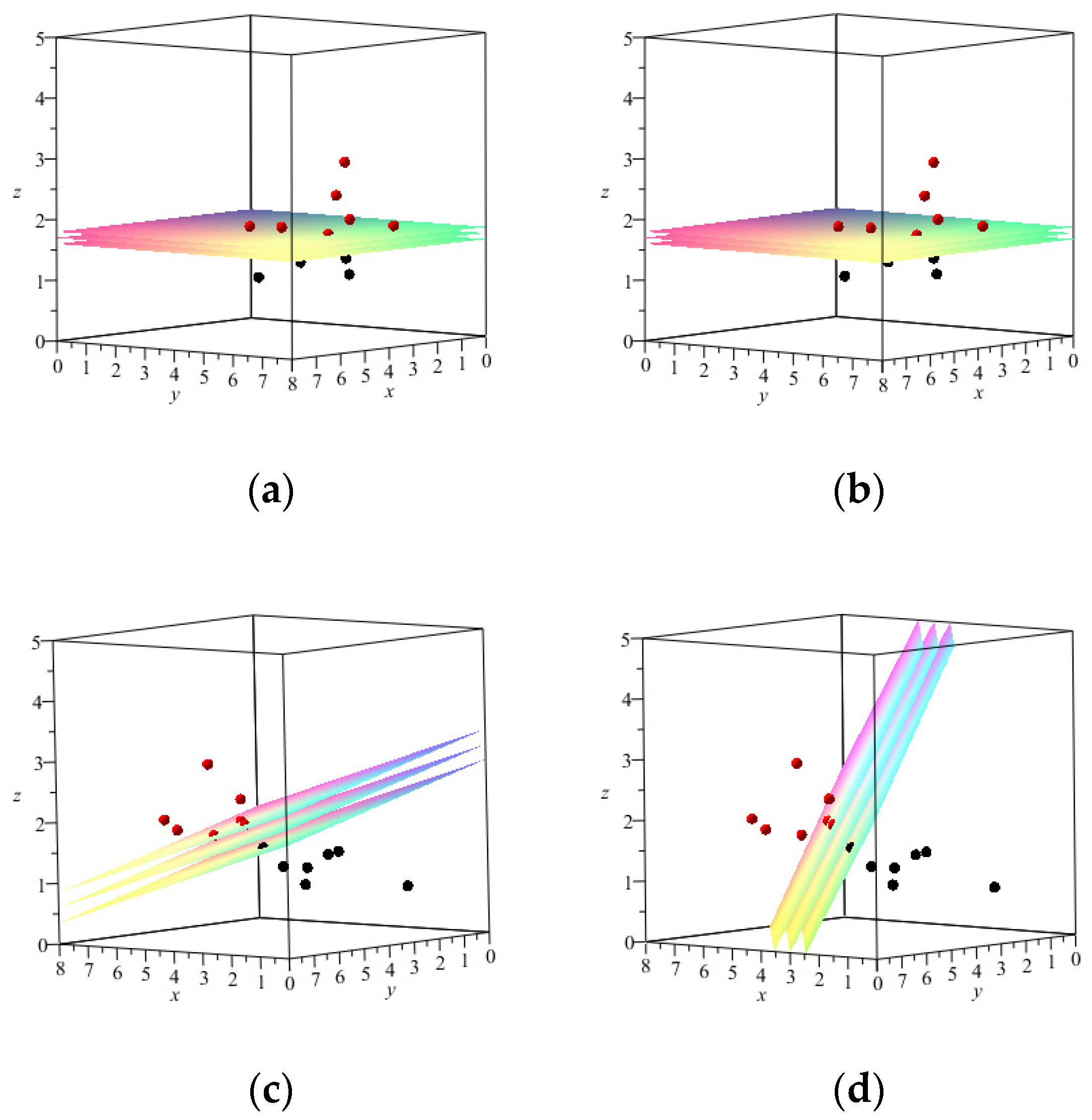
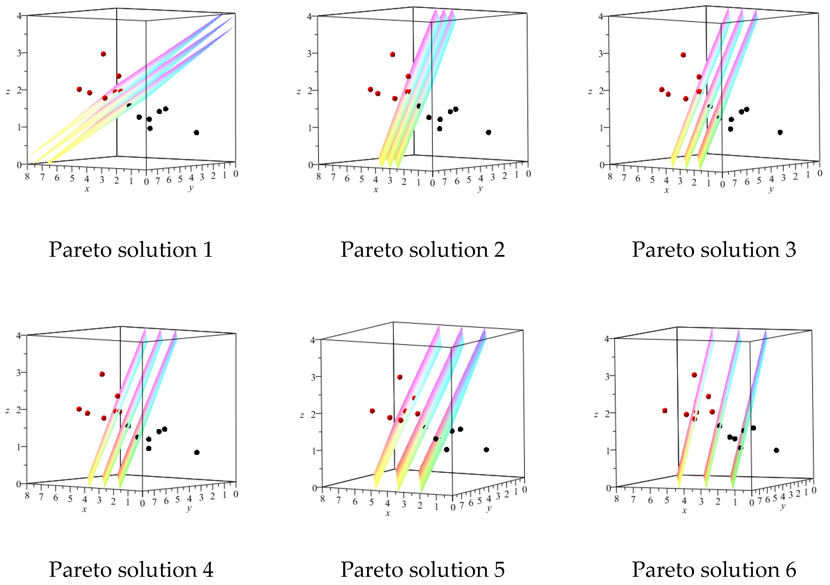
We used the dataset for our MOP models to obtain 100 Pareto solutions. We have considered 6 Pareto solutions out of 100 Pareto solutions obtained for each MOP for further investigation. In Figure 2, Figure 3, Figure 4 and Figure 5, we have considered a suitable viewing angle for each specific sample (6 Pareto solutions) to have a better view of the separating hyperplanes for MOP models. Additionally, in

Table 2. The results of $l_1$ MOP model for Test Problem 1.

Pareto Solution	w_1	w_2	w_3	${‖\mathit{w}‖}_1$	Error Value	Correctness
1	$-$0.7400	$-0.4933$	$-3.9470$	$5.1803$	0	$100.00$%
2	$-0.7048$	$-0.4699$	$-3.7590$	$4.9336$	0	$100.00$%
$3$	$-0.4405$	$-0.2937$	$-2.3494$	$3.0835$	$0.8253$	$92.86$%
$4$	$-0.8068$	$-0.1502$	$-1.0164$	$1.9734$	$1.3569$	$85.72$%
5	$-0.7739$	$-0.3108$	$-0.0254$	$1.1101$	$2.9710$	$64.29$%
6	$-0.7405$	$-0.2462$	0	$0.9867$	$3.4620$	$50.00$%

,

Table 3. The results of $l_2$ multi-objective model for Test Problem 1.

Pareto Solution	w_1	w_2	w_3	${‖\mathit{w}‖}_1$	Error Value	Correctness
1	$-1.0146$	$-0.7756$	$-3.5230$	$5.3132$	0	100.00%
2	$-1.7660$	$-1.5736$	$-1.8893$	$5.2289$	0	100.00%
$3$	$-1.0196$	$-0.9085$	$-1.0908$	$3.0189$	$0.9055$	92.86%
$4$	$-0.9476$	$-0.7882$	$-0.9616$	$2.6974$	$1.0317$	85.72%
5	$-0.7108$	$-0.4092$	$-0.7411$	$1.8611$	$1.6263$	78.57%
6	$-0.6313$	$-0.3030$	$-0.3473$	$1.2816$	$2.7562$	57.14%

,

Table 4. The results of the BM-SVM multi-objective model for Test Problem 1.

Pareto Solution	w_1	w_2	w_3	${‖\mathit{w}‖}_1$	Error Value	Correctness
1	$-0.7500$	$-0.5000$	$-4.0000$	5.25000	0	100.00%
2	$-0.0460$	0	$-9.7375$	9.7835	0	100.00%
$3$	0	0	$-8.5929$	8.5929	0	100.00%
$4$	$-6.5340$	0	0	6.5340	0.7374	92.86%
5	0	0	$-5.0000$	5.0000	1.4748	85.71%
6	0	0	$-4.0000$	4.0000	1.6000	78.57%

and

Table 5. The results of the SVM₀ multi-objective model for Test Problem 1.

Pareto Solution	w_1	w_2	w_3	${‖\mathit{w}‖}_1$	Error Value	Correctness
1	$-0.7500$	$-0.5000$	$-4.0000$	5.2500	0	100.00%
2	$-5.0000$	0	$-2.5000$	7.5000	0	100.00%
$3$	0	0	$-9.8603$	9.8603	0	100.00%
$4$	0	0	$-7.2591$	7.2591	0.5481	92.86%
5	$-6.5625$	0	0	6.5625	1.2386	92.86%
6	0	0	$-5.0000$	5.0000	2.1090	78.57%

, the results obtained for the same Pareto optimal solutions are displayed.

In Table 2 for the $l_1$ MOP, the value of ${‖w‖}_1$ gradually decreases in the solutions while the error value increases.

For example, in the first and second Pareto solutions, a smaller value for the ${‖w‖}_1$ (with an error value equal to zero) has been achieved compared to the results of the single-objective $l_1$, presented in Table 1. In the sixth Pareto solution, one of the components of the vector $w$ is equal to zero, but the error has increased.

In Table 3 for the $l_2$ MOP model, in the first and second Pareto solutions, a smaller value for the ${‖w‖}_1$ has been achieved (with an error value equal to zero) compared to the results of the single-objective $l_2$ problem, presented in Table 1.

In Table 4 for the BM-SVM MOP model, in the third Pareto solution, two components of the vector $w$ are non-zero (with an error value equal to zero) while compared to the results of the single-objective model, presented in Table 1, a smaller value for the ${‖w‖}_1$ has been achieved.

For the SVM₀ MOP model, as shown in Figure 5 and Table 5, in the third Pareto solution, two components of the vector $w$ are non-zero (with an error value equal to zero) while compared to the results of the single-objective model, presented in Table 1, a smaller value for the ${‖w‖}_1$ has been achieved.

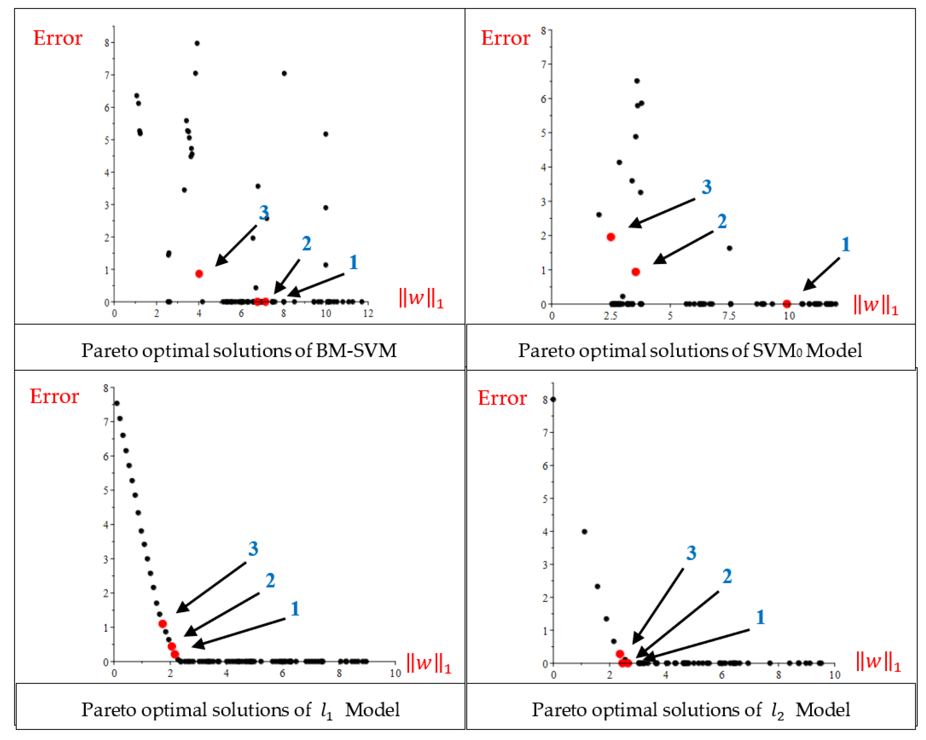
The projection of all Pareto solutions (in the space of Error (Vertical axis) and $l_1$ norm (Horizontal axis)) obtained from multi-objective models (BM-SVM, SVM₀, $l_1$, $l_2$) are shown in Figure 6. Additionally, the run time (second) of $l_1$, $l_2$, BM-SVM and SVM₀ multi-objective models, respectively, are 227.906, 269.468, 901.235, and 1236.515 for obtaining 100 Pareto optimal solutions. The lowest run time was related to model $l_1$, but as the results of the previous tables, models BM-SVM and SVM₀ have performed better in terms of the minimum number of non-zero components of the normal vector of the separator hyperplane.

Test Problem 2.

The number of samples is 12, and the number of features is 4 in this test problem. Suppose that we have two sets as follows:

$$A=\left\{\left[1.5, 4.2, 1, 2\right], \left[1.9, 4.6, 1.5, 1.5\right], \left[1.8, 4.5, 1.6, 1.9\right],\right.\left[1.5, 4.3, 1.2, 1.8\right],\left. \left[1.2, 4.5, 1.6, 1.6\right], [1.7, 4.5, 1.4, 2]\right\}$$

$$B=\left\{\left[2.2, 6, 3, 2.1\right], \left[2.6, 5, 2, 2.3\right], \left[4, 4.7, 1.7, 2.5\right],\right.[3.2, 4.5, 2.1, 2.3],\left.[3.5, 5.3, 2.5, 3.1], [2.1, 5.6, 2.5, 3.2]\right\}$$

The results are shown in

Table 6. The results of single-objective models for Test Problem 2.

Method	w_1	w_2	w_3	w_4	${‖\mathit{w}‖}_1$	Error Value	Correctness
BM-SVM	$-10.00$	0	0	0	10.00	0	100.00%
SVM0 Model	$-10.00$	0	0	0	10.00	0	100.00%
$l_1$Model	$-1.7886$	$-0.4878$	$-0.3252$	$-0.4878$	3.0894	0	100.00%
$l_2$Model	$-1.3223$	$-0.8264$	$-0.6612$	$-0.6612$	3.4711	0	100.00%

. The single-objective models all provide the correct set separator (that is, the error of all these models is zero). The vector $w$ returned by BM-SVM and SVM₀ methods has just one non-zero component, but $l_1$ and $l_2$ return a vector $w$ where all components are non-zero.

Pareto optimal solutions obtained from MOP models are depicted in Figure 7. In this figure, the horizontal axis represents the value of $l_1$ norm of vector $w$, and the vertical axis represents the error level. To clarify the discussion, in Figure 8a, the Pareto frontier of the BM-SVM multi-objective model is displayed in the space of the objective functions of this model for Test Problem 2. In Figure 8b the projection of this Pareto frontier in the space of Error (vertical axis) and $l_1$-norm (horizontal axis) is displayed.

We have considered only three Pareto solutions out of the 100 Pareto optimal solutions obtained for each MOP model that seemed more interesting for consideration. The results are displayed in

Table 7. The results of some Pareto solutions of BM-SVM multi-objective model for the dataset of Test Problem 2.

Pareto Solution	w_1	w_2	w_3	w_4	${‖\mathit{w}‖}_1$	Error Value	Correctness
1	0	0	$-4.8920$	0	4.8920	3.4020	75.00%
2	0	0	$-2.2222$	0	2.2222	7.6788	66.67%
3	0	0	$-5.3441$	0	5.3441	18.3710	58.33%

,

Table 8. The results of some Pareto solutions of the SVM₀ multi-objective model for the dataset of Test Problem 2.

Pareto Solution	w_1	w_2	w_3	w_4	${‖\mathit{w}‖}_1$	Error Value	Correctness
1	$-1.6949$	$-2.0339$	0	0	3.7288	0	100.00%
2	$-7.2008$	0	0	0	7.2008	0.5598	91.67%
3	0	0	$-4.6410$	0	4.6410	1.6795	83.33%

,

Table 9. The results of some Pareto solutions of $l_1$ multi-objective model for the dataset of Test Problem 2.

Pareto Solution	w_1	w_2	w_3	w_4	${‖\mathit{w}‖}_1$	Error Value	Correctness
1	$-0.7279$	$\cong 0$	$-0.9160$	$-0.4826$	2.1265	1.0984	66.67%
2	$-0.6897$	$\cong 0$	$-0.8314$	$-0.2927$	1.8138	1.8273	58.33%
3	$-0.8121$	$\cong 0$	$-0.7514$	$\cong 0$	1.5636	2.5273	50.00%

and

Table 10. The results of some Pareto solutions of $l_2$ multi-objective model for the dataset of Test Problem 2.

Pareto Solution	w_1	w_2	w_3	w_4	${‖\mathit{w}‖}_1$	Error Value	Correctness
1	$-0.9504$	$-0.3632$	$-0.5770$	$-0.5682$	2.4588	0.6000	83.33%
2	$-0.6877$	$-0.4267$	$-0.6012$	$-0.4909$	2.2065	1.2000	66.66%
3	$-0.5831$	$-0.3852$	$-0.5331$	$-0.4354$	1.9368	1.8000	58.33%

.

For the BM-SVM MOP model, as shown in Table 7, for all Pareto solutions that are considered, three components of vector $w$ is equal to zero, and in each solution, the smaller value for ${‖w‖}_1$ has been achieved, but the errors are not equal to zero.

As shown in Table 8 for the SVM₀ MOP model, in the first Pareto solution, two components of vector $w$ is equal to zero, and in the two other Pareto solutions, three components of vector $w$ is equal to zero, but the error value is non-zero.

As shown in Table 9, in the $l_1$ MOP model, for all Pareto solutions, one component of the vector $w$ is equal to zero but with non-zero error.

As shown in Table 10 for the $l_2$ MOP model, in all Pareto solutions which are considered, all components of the vector $w$ are non-zero.

The run time (second) of $l_1$, $l_2$, BM-SVM and SVM₀ multi-objective models, respectively, are 885.031, 418.578, 133.594, and 546.472 for obtaining 100 Pareto optimal solutions. The lowest run time was related to model BM-SVM. Additionally, as the results of the previous tables, models BM-SVM and SVM₀ have performed better in terms of the minimum number of non-zero components of the normal vector of the separator hyperplane.

Test Problem 3.

The number of samples is 8, and the number of features is 5 in this test problem. Suppose that we have two sets as follows:

$$\begin{array}{c}A=\left\{[2.3, 3.5, 1, 2.7, 1], [2.8, 3.6, 1.5, 2.5, 1.1], [2, 4.9, 1.6, 2.4, 1.2], [2.5, 3.9, 1.8, 2, 1.3]\right\},\\ B=\left\{[3.1, 5.6, 3, 3.1, 2], [3.6, 4.6, 2, 3.3, 2.1], [4, 5, 1.7, 2.9, 2.2], [3.2, 4.2, 2.3, 2.5, 2.4]\right\}\end{array}$$

All single-objective models provide the correct separator. The vector $w$ returned by BM-SVM and SVM₀ has just one non-zero component, but the $l_1$ and $l_2$ return a vector $w$ where components are all non-zero. The results are depicted in

Table 11. The results of Test Problem 3 for single-objective models.

Method	w_1	w_2	w_3	w_4	w_5	${‖\mathit{w}‖}_1$	Error Value	Correctness
BM-SVM	0	0	0	0	$-8.3334$	8.3334	0	100.00%
SVM0 Model	0	0	0	0	$-10.00$	10.00	0	100.00%
$l_1$Model	$-0.1892$	$-0.0946$	$-0.2270$	$-0.4541$	$-1.3623$	2.3273	0	100.00%
$l_2$Model	$-0.6114$	$-0.2620$	$-0.4367$	$-0.4367$	$-0.9607$	2.7074	0	100.00%

.

Pareto solutions obtained from MOP models are shown in Figure 9. We have considered only three Pareto solutions that seemed more interesting out of the 100 Pareto optimal solutions obtained for each MOP model. The results are shown in

Table 12. The results of some Pareto solutions of BM-SVM multi-objective model for the dataset of Test Problem 3.

Pareto Solution	w_1	w_2	w_3	w_4	w_5	${‖\mathit{w}‖}_1$	Error Value	Correctness
1	0	0	0	0	$-7.1575$	7.1575	0	100.00%
2	$-6.7742$	0	0	0	0	6.7742	0	100.00%
3	0	0	0	0	$-4.0209$	4.0209	0.8613	87.50%

,

Table 13. The results of some Pareto solutions of the SVM₀ multi-objective model for the dataset of Test Problem 3.

Pareto Solution	w_1	w_2	w_3	w_4	w_5	${‖\mathit{w}‖}_1$	Error Value	Correctness
1	0	0	0	0	$-$9.9147	9.9147	0	100.00%
2	$-$3.5484	0	0	0	0	3.5484	0.9355	87.50%
3	0	0	0	0	$-$2.5000	2.5000	1.9528	75.00%

,

Table 14. The results of some Pareto solutions of $l_1$ multi-objective model for the dataset of Test Problem 3.

Pareto Solution	w_1	w_2	w_3	w_4	w_5	${‖\mathit{w}‖}_1$	Error Value	Correctness
1	$-0.6347$	$-0.2952$	$-0.0858$	$\cong 0$	$-1.1541$	2.1699	0.2064	75.00%
2	$-0.6302$	$-0.2470$	$\cong 0$	$-0.0039$	$-1.1801$	2.0612	0.4369	62.50%
3	$-0.3035$	$-0.0437$	$\cong 0$	$\cong 0$	$-1.3887$	1.7359	1.0963	50.00%

and

Table 15. The results of some Pareto solutions of $l_2$ multi-objective model for the dataset of Test Problem 3.

Pareto Solution	w_1	w_2	w_3	w_4	w_5	${‖\mathit{w}‖}_1$	Error Value	Correctness
1	$-0.2549$	$-0.1032$	$-0.2135$	$-0.7962$	$-1.2810$	2.6489	0	100.00%
2	$-0.2120$	$-0.0556$	$-0.3538$	$-0.6104$	$-1.2298$	2.4616	0	100.00%
3	$-0.5363$	$-0.2690$	$-0.3751$	$-0.3867$	$-0.8051$	2.3721	0.2774	87.50%

.

For BM-SVM MOP, as shown in Table 12, for the first and second Pareto solutions, four components of vector $w$ are equal to zero, and the error values are zero. Additionally, compared to the results of the single-objective model, a smaller value for the ${‖w‖}_1$ has been achieved.

For the SVM₀ MOP model, as shown in Table 13, for the first Pareto solution, four components of vector $w$ are equal to zero, and the error value is equal to zero, for the second and third Pareto solutions, while the error value is non-zero, four components of vector $w$ are equal to zero.

For the $l_1$ MOP model, as shown in Table 14, one component of vector $w$ is equal to zero, with a non-zero error.

For the $l_2$ MOP model, as shown in, for all Pareto solutions, all components of vector $w$ are non-zero.

The run time (second) of $l_1$, $l_2$, BM-SVM, and SVM₀ multi-objective models, respectively, are 102.500, 134.188, 239.953, and 576.343 for obtaining 100 Pareto optimal solutions. The lowest run time was related to $l_1$ model. Additionally, as the results of the previous tables, models BM-SVM and SVM₀ have performed better in terms of the minimum number of non-zero components of the normal vector of the separator hyperplane.

5. Conclusions

The design of linear Support Vector Machine (SVM) classification techniques is generally a multi-objective optimization that requires finding appropriate trade-offs between several objectives, such as misclassified training data (classification error) and the number of non-zero elements of the separator hyperplane. We proposed multi-objective binary classification problems to show the advantages of considering these problems for sparse optimization in linear SVM classification techniques. The results of the proposed classification methods in single-objective and multi-objective forms are reported on several datasets. The results showed that by using multi-objective models, we can choose a more appropriate separating hyperplane. By using multi-objective models (especially BM-SVM and SVM₀ multi-objective models), separator hyperplanes have been obtained with the minimum possible error and, at the same time, the minimum number of non-zero components of the normal vector.

References

1. Jin, Y.; Sendhoff, B. Pareto-Based Multiobjective Machine Learning: An Overview and Case Studies. IEEE Trans. Syst. Man Cybern. Part C (Appl. Rev.) 2008, 38, 397–415. [Google Scholar] [CrossRef]
2. Suttorp, T.; Igel, C. Multi-Objective Optimization of Support Vector Machines. In Multi-Objective Machine Learning; Jin, Y., Ed.; Studies in Computational Intelligence; Springer: Berlin/Heidelberg, Germany, 2006; Volume 16. [Google Scholar] [CrossRef]
3. Zoltan, Z.; Kalmar, Z.; Szepesvari, C. Multi-criteria reinforcement learning. Proc. Int. Conf. Mach. Learn. 1998, 98, 197–205. [Google Scholar]
4. Coleman, T.F. (Ed.) Large Sparse Numerical Optimization; Springer: Berlin/Heidelberg, Germany, 1984. [Google Scholar] [CrossRef]
5. Zhao, Y.B. Sparse Optimization Theory and Methods; CRC Press: Boca Raton, FL, USA, 2018. [Google Scholar] [CrossRef]
6. Van Zyl, J.P.; Engelbrecht, A.P. Set-Based Particle Swarm Optimisation: A Review. Mathematics 2023, 11, 2980. [Google Scholar] [CrossRef]
7. Zitzler, E. Evolutionary Algorithms for Multiobjective Optimization: Methods and Applications; Shaker: Ithaca, NY, USA, 1999; Volume 63. [Google Scholar]
8. Collette, Y.; Siarry, P. Multiobjective optimization: Principles and case studies. In Decision Engineering; Springer: Berlin/Heidelberg, Germany, 2003. [Google Scholar]
9. Das, I.; Dennis, J.E. A closer look at drawbacks of minimizing weighted sums of objectives for Pareto set generation in multicriteria optimization problems. Struct. Optim. 1997, 14, 63–69. [Google Scholar] [CrossRef]
10. Teixeira, R.A.; Braga, A.P.; Takahashi, R.H.C.; Saldanha, R.R. Improving generalization of MLPs with multi-objective optimization. Neurocomputing 2000, 35, 189–194. [Google Scholar] [CrossRef]
11. Deb, K. Multi-objective optimisation using evolutionary algorithms: An introduction. In Multi-Objective Evolutionary Optimisation for Product Design and Manufacturing; Springer: London, UK, 2011; pp. 3–34. [Google Scholar]
12. Sawaragi, Y.; Nakayama, H.; Tanino, T. Theory of multiobjective optimization. In Mathematics in Science and Engineering; Elsevier: Amsterdam, The Netherlands, 1985; Volume 176. [Google Scholar]
13. Chankong, V.; Haimes, Y. Optimization-based methods for multiobjective decision-making: An overview. Large Scale Syst. 1983, 5, 1–33. [Google Scholar]
14. Coello Coello, C.A.; Van Veldhuizen, D.A.; Lamont, G.B. Evolutionary Algorithms for Solving Multi-Objective Problems; Kluwer Academic Publishers: Dordrecht, The Netherlands, 2002. [Google Scholar]
15. Pareto, V.; Bonnet, A. Manuel D’économie Politique; Giard, V., Brière, E., Eds.; Bibliothèque Internationale D’économie Politique: Paris, France, 1909. [Google Scholar]
16. Lopez-Ibanez, M.; Dubois-Lacoste, J.; Stutzle, T.; Birattari, M. The Irace Package, Iterated Race for Automatic Algorithm Configuration; Technical Report TR/IRIDIA/2011-004, IRIDIA; Université Libre de Bruxelles: Bruxelles, Belgium, 2011. [Google Scholar]
17. Lang, M.; Kotthaus, H.; Marwedel, P.; Weihs, C.; Rahnenführer, J.; Bischl, B. Automatic model selection for high-dimensional survival analysis. J. Stat. Comput. Simul. 2015, 85, 62–76. [Google Scholar] [CrossRef]
18. Jones, D.R. A taxonomy of global optimization methods based on response surfaces. J. Glob. Optim. 2001, 21, 345–383. [Google Scholar] [CrossRef]
19. Thornton, C.; Hutter, F.; Hoos, H.H.; Leyton-Brown, K. August. Auto-WEKA: Combined selection and hyperparameter optimization of classification algorithms. In Proceedings of the 19th ACM SIGKDD International Conference on Knowledge Discovery and Data Mining, Ser. KDD ’13, Chicago, IL, USA, 11–14 August 2013; ACM: New York, NY, USA, 2013; pp. 847–855. [Google Scholar]
20. Koch, P.; Bischl, B.; Flasch, O.; Bartz-Beielstein, T.; Weihs, C.; Konen, W. Tuning and evolution of support vector kernels. Evol. Intell. 2012, 5, 153–170. [Google Scholar] [CrossRef]
21. Jin, Y. Surrogate-assisted evolutionary computation: Recent advances and future challenges. Swarm Evol. Comput. 2011, 1, 61–70. [Google Scholar] [CrossRef]
22. Horn, D.; Demircioğlu, A.; Bischl, B.; Glasmachers, T.; Weihs, C. A comparative study on large scale kernelized support vector machines. Adv. Data Anal. Classif. 2018, 12, 867–883. [Google Scholar]
23. Jin, Y. (Ed.) Multi-Objective Machine Learning; Springer Science & Business Media: Berlin/Heidelberg, Germany, 2006; Volume 16. [Google Scholar]
24. Everson, R.M.; Fieldsend, J.E. Multi-class {ROC} analysis from a multi-objective optimisation perspective. Pattern Recognit. Lett. 2006, 27, 918–927. [Google Scholar]
25. Graning, L.; Jin, Y.; Sendhoff, B. Generalization improvement in multi-objective learning. In Proceedings of the 2006 IEEE International Joint Conference on Neural Network Proceedings, Vancouver, BC, Canada, 16–21 July 2006; IEEE: New York, NY, USA, 2006; pp. 4839–4846. [Google Scholar]
26. Law, M.H.; Topchy, A.P.; Jain, A.K. Multiobjective data clustering. In Proceedings of the 2004 IEEE Computer Society Conference on Computer Vision and Pattern Recognition, Washington, DC, USA, 27 June–2 July 2004; IEEE: New York, NY, USA, 2004; Volume 2, p. II. [Google Scholar]
27. Liu, G.P.; Kadirkamanathan, V. Learning with multi-objective criteria. In Proceedings of the 1995 Fourth International Conference on Artificial Neural Networks, Perth, WA, Australia, 27 November–1 December 1995; pp. 53–58. [Google Scholar]
28. Bi, J. Multi-objective programming in SVMs. In Proceedings of the 20th International Conference on Machine Learning, Washington, DC, USA, 21–24 August 2003; pp. 35–42. [Google Scholar]
29. Igel, C. Multi-objective model selection for support vector machines. In Evolution Multi-Criterion Optimization Lecture Notes in Computer Science; Springer: New York, NY, USA, 2005; Volume 3410, pp. 534–546. [Google Scholar]
30. Nakayama, H.; Asada, T. Support vector machines formulated as multi-objective linear programming. In Proceedings of the ICOTA, Hong Kong, 15–17 December 2001; pp. 1171–1178. [Google Scholar]
31. Bernado-Manssilla, E.; Garrell-Guii, J. MOLeCS: Using multiobjective evolutionary algorithms for learning. In Proceedings of the EMO 2001 Lecture Notes in Computer Science, Zurich, Switzerland, 7–9 March 2001; Springer: New York, NY, USA, 2001; Volume 1993, pp. 696–710. [Google Scholar]
32. Zhang, Y.; Rockett, P.I. Evolving optimal feature extraction using multi-objective genetic programming: A methodology and preliminary study on edge detection. In Proceedings of the Genetic and Evolutionary Computation Conference, Washington, DC, USA, 25–29 June 2005; pp. 795–802. [Google Scholar]
33. Ishibuchi, H.; Nakashima, T.; Murata, T. Three-objective genetics-based machine learning for linguistic rule extraction. Inf. Sci. 2001, 136, 109–133. [Google Scholar]
34. Van Moffaert, K.; Nowé, A. Multi-objective reinforcement learning using sets of Pareto dominating policies. J. Mach. Learn. Res. 2014, 15, 3483–3512. [Google Scholar]
35. Cordon, O.; Herrera, F.; del-Jesus, M.; Villar, P. A multi-objective genetic algorithm for feature selection and granularity learning in fuzzy-rule based classification systems. In Proceedings of 9th IFSA World Congress and 20th NAFIPS International Conference, Vancouver, BC, Canada, 25–28 July 2001; Volume 3, pp. 1253–1258. [Google Scholar]
36. Oliveira, L.S.; Sabourin, R.; Bortolozzi, F.; Suen, C.Y. Feature selection for ensembles: A hierarchical multi-objective genetic algorithm approach. In Proceedings of the Seventh International Conference on Document Analysis and Recognition, Edinburgh, UK, 3–6 August 2003; IEEE: New York, NY, USA; pp. 676–680. [Google Scholar]
37. Handl, J.; Knowles, J. Exploiting the Tradeoff—The Benefits of Multiple Objectives in Data Clustering, Evolutionary Multi-Criterion Optimization Lecture Notes in Computer Science; Springer: New York, NY, USA, 2005; Volume 3410, pp. 547–560. [Google Scholar]
38. Jin, Y.; Sendhoff, B. Alleviating catastrophic forgetting via multiobjective learning. In Proceedings of International Joint Conference on Neural Network, Vancouver, BC, Canada, 16–21 July 2006; pp. 6367–6374. [Google Scholar]
39. Kokshenev, I.; Braga, A.P. An efficient multi-objective learning algorithm for RBF neural network. Neurocomputing 2010, 73, 2799–2808. [Google Scholar]
40. Torres, L.C.B.; Castro, C.L.; Braga, A.P. A computational geometry approach for Pareto-optimal selection of neural networks. In Proceedings of the International Conference on Artificial Neural Networks (ICANN), Lausanne, Switzerland, 11–14 September 2012; pp. 100–107. [Google Scholar]
41. Teixeira, R.; Braga, A.P.; Saldanha, R.; Takahashi, R.H.; Medeiros, T.H. The usage of golden section in calculating the efficient solution in artificial neural networks training by multi-objective optimization. In Proceedings of the International Conference on Artificial Neural Networks (ICANN), Porto, Portugal, 9–13 September 2007; Volume 4668, pp. 289–298. [Google Scholar]
42. Chankong, V.; Haimes, Y.Y. Multiobjective Decision Making: Theory and Methodology; Elsevier: Amsterdam, The Netherlands; North-Holland: New York, NY, USA, 1983; Volume 8. [Google Scholar]
43. Nisbet, R.; Elder, J.; Miner, G.D. Handbook of Statistical Analysis and Data Mining Applications; Academic Press: Cambridge, MA, USA, 2009. [Google Scholar]
44. Yang, X.S. Introduction to Algorithms for Data Mining and Machine Learning; Academic Press: Cambridge, MA, USA, 2019. [Google Scholar]
45. Zhao, Y.; Cen, Y. Data Mining Applications with R; Academic Press: Cambridge, MA, USA, 2013. [Google Scholar]
46. Rinaldi, F. Mathematical Programming Methods for Minimizing the Zero-Norm over Polyhedral Sets. 2009, Sapienza, University of Rome. Available online: https://citeseerx.ist.psu.edu/viewdoc/download?doi=10.1.1.726.794&rep=rep1&type=pdf (accessed on 18 August 2023).
47. Rumelhart, D.E.; Hinton, G.E.; Williams, R.J. Learning representations by back-propagating errors. Nature 1986, 323, 533–536. [Google Scholar]
48. Haykin, S. Neural Networks: A Comprehensive Foundation, 2nd ed.; Prentice-Hall: New York, NY, USA, 1999. [Google Scholar]
49. Bradley, P.S.; Mangasarian, O.L. Feature selection via concave minimization and support vector machines, Machine Learning Proceedings of the Fifteenth International Conference (ICML 1998), Madison, WI, USA, 24–27 July 1998; Shavlik, J., Ed.; Morgan Kaufmann: San Francisco, CA, USA, 1998; pp. 82–90. [Google Scholar]
50. Bennett, K.P.; Blue, J.A. A support vector machine approach to decision trees. In Proceedings of the IEEE International Joint Conference on Neural Networks Proceedings. IEEE World Congress on Computational Intelligence (Cat. No.98CH36227), Anchorage, AK, USA, 4–9 May 1998; Volume 3, pp. 2396–2401. [Google Scholar]
51. Vapnik, V. The Nature of Statistical Learning Theory, 2nd ed.; Springer Science & Business Media: Berlin/Heidelberg, Germany, 1999. [Google Scholar]
52. Rinaldi, F.; Schoen, F.; Sciandrone, M. Concave programming for minimizing the zero-norm over polyhedral sets. Comput. Optim. Appl. 2010, 46, 467–486. [Google Scholar] [CrossRef]
53. Bishop, C.M. Neural Networks for Pattern Recognition; Oxford University Press: New York, NY, USA, 1995. [Google Scholar]
54. Gaudioso, M.; Gorgone, E.; Hiriart-Urruty, J.B. Feature selection in SVM via polyhedral k-norm. Optim. Lett. 2020, 14, 19–36. [Google Scholar] [CrossRef]
55. Mangasarian, O.L. Machine learning via polyhedral concave minimization. In Applied Mathematics and Parallel Computing: Festschrift for Klaus Ritter; Physica-Verlag HD: Heidelberg, Germany, 1996; pp. 175–188. [Google Scholar]
56. Gaudioso, M.; Gorgone, E.; Labbé, M.; Rodríguez-Chía, A.M. Lagrangian relaxation for SVM feature selection. Comput. Oper. Res. 2017, 87, 137–145, ISSN 0305-0548. [Google Scholar] [CrossRef]
57. Gaudioso, M.; Giallombardo, G.; Miglionico, G.; Bagirov, A.M. Minimizing nonsmooth DC functions via successive DC piecewise affine approximations. J. Glob. Optim. 2018, 71, 37–55. [Google Scholar]
58. Pirouz, B.; Gaudioso, M. New Mixed Integer Fractional Programming Problem for Sparse Optimization. In Proceedings of the ODS 2021: International Conference on Optimization and Decision Sciences, Rome, Italy, 19 September 2021; Available online: http://www.airoconference.it/ods2021/images/ODS2021_Conference_Program_web_v4.pdf (accessed on 18 August 2023).
59. Pirouz, B.; Gaudioso, M. A Multi-Objective Programming Problem for Sparse Optimization with application in SVM feature selection. In Proceedings of the ODS 2022: International Conference on Optimization and Decision Sciences, Firenze, Italy, 25 August 2024. [Google Scholar]
60. Pirouz, B.; Gaudioso, M. New mixed integer fractional programming problem and some multi-objective models for sparse optimization. Soft Comput. 2023, 1–12. [Google Scholar] [CrossRef]
61. Ehrgott, M. Multicriteria Optimization, 2nd ed.; Springer: Berlin/Heidelberg, Germany, 2005. [Google Scholar]
62. Mavrotas, G. Effective implementation of the ε-constraint method in multi-objective mathematical programming problems. Appl. Math. Comput. 2009, 213, 455–465. [Google Scholar] [CrossRef]
63. Pirouz, B.; Khorram, E. A Computational Approach Based on the epsilon-Constraint Method in Multi-Objective Optimization Problems. In Advances and Applications in Statistics; Pushpa Publishing House: Allahabad, India, 2016. [Google Scholar] [CrossRef]
64. Pirouz., B.; Ramezani Paschapari, J. A Computational Algorithm Based on Normalization for Constructing the Pareto Front of Multiobjective Optimization Problems. In Proceedings of the 5th International Conference on Industrial and Systems Engineering, Mashhad, Iran, 4 September 2019. [Google Scholar]
65. Pinter, J.D.; Linder, D.; Chin, P. Global optimization toolbox for maple: An introduction with illustrative applications. Optim. Methods Softw. 2006, 21, 565–582. [Google Scholar] [CrossRef]
66. Maplesoft. Available online: https://www.maplesoft.com/support/help/maple/view.aspx?path=GlobalOptimization%2FGlobalSolve#info (accessed on 18 August 2023).
Figure 1. The result of Separator Hyperplanes in single-objective models for Test Problem 1. (a) Separator Hyperplanes of BM-SVM. (b) Separator Hyperplanes of SVM0. (c) Separator Hyperplanes of l 1 . (d) Separator Hyperplanes of l 2 .
Mathematics 11 03721 g001
Figure 2. Some results of Separator Hyperplanes in l 1 MOP model for Test Problem 1.
Mathematics 11 03721 g002
Figure 3. Some results of Separator Hyperplanes in l 2 MOP model for Test Problem 1.
Mathematics 11 03721 g003
Figure 4. Some results of Separator Hyperplanes in BM-SVM MOP model for Test Problem 1.
Mathematics 11 03721 g004
Figure 5. Some results of Separator Hyperplanes in SVM0 MOP model for Test Problem 1.
Mathematics 11 03721 g005
Figure 6. The projection of Pareto solutions (in the space of error and l_1 norm) obtained from multi-objective models (BM-SVM, SVM0, l 1 and l 2 models) for the dataset of Test Problem 1.
Mathematics 11 03721 g006
Figure 7. The projection of Pareto solutions (in the space of Error and l_1 norm) obtained from multi-objective models for the dataset of Test Problem 2.
Mathematics 11 03721 g007
Figure 8. The Pareto frontier of the BM-SVM multi-objective model and its projection for Test Problem 2. (a) The Pareto solutions in the space of objective functions of the BM-SVM model for Test Problem 2. (b) The projection of Pareto solutions in the space of Error and l 1 -norm for Test Problem 2.
Mathematics 11 03721 g008
Figure 9. The projection of Pareto solutions (in the space of Error and l_1 norm) obtained from multi-objective models for the dataset of Test Problem 3.
Mathematics 11 03721 g009