Optimal Consumption and Investment Problem under 4/2-CIR Stochastic Hybrid Model

Abstract

In this paper, we investigate the optimal consumption and investment problem under the expected utility maximization criterion. It is supposed that the financial market consists of a risky asset and a risk-free asset, and the risky asset prices follow the 4/2 Cox–Ingersoll–Ross (CIR) stochastic hybrid model. The investment objective is to obtain an optimal consumption–investment strategy by maximizing the objective function. The closed-form expression of the optimal consumption–investment strategy is obtained by using optimal control theory and the corresponding Hamilton–Jacobi–Bellman (HJB) equation under the power utility function. In addition, we present a numerical example to illustrate the influence of model parameters on the optimal consumption–investment strategy.

1. Introduction

The research on the optimal consumption and investment problem can be traced back to Merton [1], and since then more and more scholars have been focusing on this problem. For example, Fleming et al. [2] studied the optimal consumption and investment problem of a single agent under the assumption that the market consists only of risk-free assets and risky assets. They gave the solution of the expected utility function dynamic programming differential equation in the case of hyperbolic absolute risk aversion (HARA) utility, and obtained the asymptotic behavior of the value function. For the intertemporal consumption and investment portfolio problem with constant opportunity and borrowing constraints, the optimal strategy can be expressed as a feedback function of current wealth under the general assumption of an agent utility function [3]. Dai et al. [4] studied the continuous-time optimal consumption and investment problem for investors with proportional transaction costs and constant relative risk aversion (CRRA) in a finite horizon, and obtained the regularity of the corresponding value function. Later, Chang et al. [5] studied the consumer investment problem with time-lagged stochastic control under the correlation of risky asset returns with historical returns, obtained a solution in a finite-dimensional space, and gave the corresponding validation theorem. In addition, Wei et al. [6] studied the optimal consumption and portfolio problem for fuzzy averse investors with recursive preferences in a complete market, and found that fuzzy aversion has a significant effect on optimal diffusion risk and jump risk. Most of the above studies of optimal consumption–investment strategies assume that the process of risky assets obeys geometric Brownian motion. However, with the in-depth study of the characteristics of the asset price, it is found that the geometric Brownian motion model does not accurately portray the real trend in asset prices, that is to say, this model cannot accurately reflect the trend in risky assets and the degree of risk, which has some influence on the investment results of the optimal consumption–investment strategy. Later, it was found that using a stochastic volatility model to describe the changing trend in investment asset prices could make up for the inaccuracy of constant volatility in describing the volatility trend in risk assets. Therefore, scholars conducted research on the optimal consumption–investment problem based on the stochastic volatility model.

Currently, the main stochastic volatility models used to study the optimal consumption–investment strategy are the Heston stochastic volatility model [7], the 3/2 stochastic volatility model [8], and the 4/2 stochastic volatility model [9]. The optimal consumption and investment problem under the Heston stochastic volatility model has been studied extensively [10,11,12,13]. However, it is found that the Heston stochastic volatility model cannot fit the extreme cases with excessive volatility, but the 3/2 stochastic volatility model, as an inverse CIR process, can make up for the deficiency of the Heston stochastic volatility. Therefore, the problem of optimal consumption and investment based on the 3/2 stochastic volatility model has attracted wide attention [14,15,16,17]. Although the 3/2 stochastic volatility model remedies the defects of the Heston stochastic volatility model, it cannot fit the low volatility of asset prices. Therefore, Grasseli [9] proposed a 4/2 stochastic volatility model with two-factor characteristics, which not only remedied the defects of the Heston stochastic volatility model but also solved the shortcomings of the 3/2 stochastic volatility model. The existing research on optimal portfolios based on the 4/2 stochastic volatility model are carried out mainly based on the mean-variance criterion and the utility maximization criterion. Zhang [18], Wang et al. [19], and Zhang [20] studied investment reinsurance, optimal investment with mispricing, and asset liability management problems, respectively, based on the 4/2 stochastic volatility model under the mean-variance criterion. In addition, the optimal investment problems for the CRRA utility function under the 4/2 stochastic volatility model are mainly studied under the utility maximization criterion (Zhang [21]), while the optimal consumption problems still need further exploration.

With the continuous changes in financial market transactions and national economic policies, the interest rate is no longer a constant. In other words, the savings, consumption and investment decisions of investors are influenced by changes in the interest rate. Therefore, the interest rate model is introduced into the research of the optimal consumption–investment strategy. For example, Noh, et al. [22] studied the problem of consumption and investment under a stochastic mixed model in infinite time and obtained the asymptotic solution of the optimal consumption–investment strategy. Escobar, et al. [23] studied the fuzzy aversion investment problem based on a mixed model of interest rate and stochastic volatility in the case of incomplete and complete markets. They found that bond investment is more sensitive to interest rate fuzziness in incomplete markets. While the effect of volatility ambiguity on the optimal portfolio is not significant, in the complete market, both volatility ambiguity and interest rate ambiguity have a significant effect on the optimal portfolio. In addition, Lin, et al. [24] studied continuous-time consumer investment strategies under interest rate uncertainty, and found that investors will exit the bond market and invest only in risky assets when interest rates decrease sufficiently. All of the above studies show that the randomness of market interest rates has a significant impact on the optimal consumption–investment strategy, that is to say, the influence of the randomness of interest rates on the optimal result should be considered when constructing the portfolio model. However, the problem of the optimal portfolio strategy based on a stochastic hybrid model mainly introduces interest rate models based on the Heston stochastic volatility model, which does not fully describe the price fluctuation trends of risky assets.

To sum up, the research on the optimal consumption–investment strategy under the stochastic hybrid model mainly has the following problems: First, the optimal investment is mainly focused on, while the optimal consumption problem is rarely discussed under the 4/2 stochastic volatility model in the literature. Secondly, under the utility maximization criterion, the influence of the interest rate on the optimal consumption–investment strategy mainly focuses on the Heston stochastic volatility model, which does not provide a comprehensive description of market volatility. Therefore, this paper considers introducing the CIR interest rate model into the 4/2 stochastic volatility model with two-factor characteristics, and constructing a stochastic hybrid consumption and portfolio model with risky asset prices satisfying the 4/2-CIR process, which can improve the fitting degree of the risky asset model to the financial market and obtain the optimal consumption–investment strategy. Then, the problem of optimal consumption and investment is studied based on the 4/2-CIR stochastic hybrid model under the assumption that there is only one risk-free asset and one risky asset in the market. We also obtained analytical expressions of the optimal consumption–investment strategy, and value functions under the power utility function by solving the stochastic differential equations (SDEs). In addition, the influence of the main parameters of the 4/2-CIR stochastic hybrid model on the optimal consumption–investment strategy is analyzed.

This paper is structured as follows: In Section 2, we construct a 4/2-CIR stochastic hybrid model and formulate the utility-maximizing portfolio problem. The solution of the HJB equation is given under the power utility function and an expression for the optimal consumption–investment strategy is obtained in Section 3. In Section 4, we present a numerical example to illustrate the effect of model parameters on the optimal consumption–investment strategy. The conclusions are given in Section 5.

2. The Model

In this section, we assume that $T>0$ is a given and fixed time of decision making and $(\Omega ,\mathcal{F},{\left\{{\mathcal{F}}_t\right\}}_{0\le t\le T},\mathbb{P})$ is a complete probability space, where information filtration ${\left\{{\mathcal{F}}_t\right\}}_{0\le t\le T}$ is generated by three one-dimensional Brownian motions $B_t$, $B_{vt}$, and $B_{rt}$.

On the basis that the financial market is continuously traded without taking into account transaction fees and taxes, it is assumed that the market consists only of the risk-free asset $P_t$ and the risky asset $S_t$. The risk-free asset price follows the dynamics:

$$\begin{array}{c}\hfill d{P}_t=r_t{P}_{t}dt.\end{array}$$

The price of stock is defined by the following dynamics:

$$\begin{array}{c}\hfill d{S}_t=\left[r_t+\lambda \left(a{v}_t+b\right)\right]S_{t}dt+\left(a\sqrt{v_t}+\frac{b}{\sqrt{v_t}}\right)S_{t}d{B}_t,S\left(0\right)=S_0>0,\end{array}$$

where parameter $\lambda \in {\mathbb{R}}^{+}$ is the control parameter of excess return, and $a,b\in {\mathbb{R}}^{+}$. The stochastic volatility $v_t$ and the interest rate $r_t$ are defined by the Cox–Ingersoll–Ross (CIR) model:

$$\begin{array}{c}\hfill d{v}_t={\xi }_1\left({\eta }_1-v_t\right)dt+{\sigma }_1\sqrt{v_t}d{B}_{vt},v\left(0\right)=v_0>0,\end{array}$$

$$\begin{array}{c}\hfill d{r}_t={\xi }_2\left({\eta }_2-r_t\right)dt+{\sigma }_2\sqrt{r_t}d{B}_{rt},r\left(0\right)=r_0>0,\end{array}$$

where ${\xi }_i,{\eta }_i$, ${\sigma }_i\in {\mathbb{R}}^{+},(i=1,2)$ denote the mean-reversion speed, long-run mean, and volatility of the interest rate, respectively. Parameter $\rho \in (-1,1)$ is the correlation coefficient of the Brownian motions $B_t$ and $B_{vt}$. $B_{rt}$ is independent of $B_t$ and $B_{vt}$, that is, $d<B_{rt},B_t>=0,d<B_{rt}$, and $B_{vt}>=0$. In addition, the Feller conditions $2{\xi }_i{\eta }_i\ge {\sigma }_i^2(i=1,2)$ are also satisfied to keep the processes $v_t$ and $r_t$ strictly positive.

Remark 1.

Note that the short-term interest rate $r_t$ is assumed to follow the CIR process in the 4/2 stochastic volatility model, so it is called the 4/2-CIR process. Furthermore, a and b are the main control parameters of the 4/2 model. In particular, the 4/2 model can degenerate into the Heston model (Heston [7]) and the 3/2 model (Heston [8]) by taking $a=1,b=0$, and $a=0,b=1$, respectively.

Let $W_t$ denote the investment wealth of investors at moment t, and the initial wealth $W_0=w>0$. We assume that $u_t$ is the proportion of wealth invested in risky assets, and $c_t$ denotes the consumption ratio. Formally, $(c_t,u_t)$ is the trading strategy. Then, the wealth process is as follows

$$d{W}_t=W_t\left[u_t\frac{d{S}_t}{S_t}+(1-u_t)\frac{d{P}_t}{P_t}\right]-c_{t}dt.$$

Combining the equations satisfied by $S_t$ and $P_t$, the wealth process $W_t$ satisfies the following SDE:

$$d{W}_t=\left\{r_t+u_t\left[\lambda \left(a{v}_t+b\right)\right]\right\}{W}_{t}dt-c_{t}dt+u_t\left(a\sqrt{v_t}+\frac{b}{\sqrt{v_t}}\right)W_{t}d{B}_t.$$

(1)

In this paper, we investigate the problem of optimal consumption and investment on a finite horizon $[0,T]$ with the objective function

$$\begin{array}{c}\hfill J(w,v,r,t)=E\left[\alpha {\int }_t^T{e}^{-\beta s}{U}_1\left(c_s\right)ds\right.\left.+(1-\alpha )e^{-\beta T}{U}_2\left(W_T\right)\right],\forall (c,u)\in \Pi ,\end{array}$$

where $U_i(·),i=1,2$ are utility functions which satisfy $U_i^{{}^{\prime }}(·)>0$ and $U_i^{{}^{\prime \prime }}(·)<0,i=1,2$. Parameter $\beta$ is the subjective discount rate and $\alpha$ is the weight of intermediate consumption.

The investment objective is to determine the optimal consumption–investment strategy $(c_t^{*},u_t^{*})\in \Pi$ that maximizes the objective function $J(w,v,r,t)$ according to the expression of $U_1\left(c_t\right)$ and $U_2\left(W_t\right)$.

Definition 1.

(Admissible strategy). The trading strategy $(c_t,u_t)$ is called an admissible strategy if the following three conditions hold true:

(1) 

$(c_t,u_t)$ is an ${\mathcal{F}}_t$-progressively measurable process.

(2) 

$E\left[{\int }_0^T{W}_t^2{\left(a\sqrt{v_t}+\frac{b}{\sqrt{v_t}}\right)}^2{u}_t^{2}dt\right]<\infty$.

(3) 

For all $\left(W_0,v_0,r_0,t_0\right)\in {\mathbb{R}}^{+}\times {\mathbb{R}}^{+}\times {\mathbb{R}}^{+}\times \left[0,T\right]$, the SDE(1) has a classical solution and

$$\begin{array}{c}\hfill E\left[\alpha {\int }_0^T{e}^{-\beta t}{U}_1\left(c_t\right)dt+(1-\alpha )e^{-\beta T}{U}_2\left(W_T\right)\right]<\infty .\end{array}$$

3. The Optimization Problem Formulation and Solution

The investor wishes to find a trading strategy that maximizes the objective function $J(w,v,r,t)$. According to the optimal consumption and investment objectives, the value function is as follows

$$\begin{array}{c}\hfill H(w,v,r,t)=\underset{(c_{·},u_{·})}{sup}J(w,v,r,t),\end{array}$$

(2)

where $H(w,v,r,t)$ is the value function, and $(c_{·},u_{·})$ denotes the admissible strategies as given by Definition 1.

The boundary condition determined by the desired final wealth is

$$\begin{array}{c}\hfill H(w,v,r,T)=(1-\alpha )e^{-\beta T}{U}_2\left(w\right).\end{array}$$

(3)

According to the principles of dynamic programming, the HJB equation should satisfy the following:

$$\begin{array}{c}0=H_t+\left[\left(r+u_t\left[\lambda (av+b)\right]\right)w-c_t\right]H_w+{\xi }_1\left({\eta }_1-v\right)H_v+{\xi }_2\left({\eta }_2-r\right)H_r\\ +\frac{1}{2}{\sigma }_1^{2}v{H}_{vv}+\frac{1}{2}{u}_t^2{\left(a\sqrt{v}+\frac{b}{\sqrt{v}}\right)}^2{w}^2{H}_{ww}+\alpha e^{-\beta t}{U}_1\left(c_t\right)+\frac{1}{2}{\sigma }_2^{2}r{H}_{rr}\\ +u_t\rho {\sigma }_1\left(a\sqrt{v}+\frac{b}{\sqrt{v}}\right)w\sqrt{v}{H}_{wv},\end{array}$$

(4)

where $H_t,H_v,H_{vv},H_r,H_{rr},H_w,H_{ww},$ and $H_{wv}$ denote the first and second partial derivatives of $H(w,v,r,t)$ with respect to $t,v,r,$ and w, respectively.

The first-order maximizing conditions for the trading strategy are

$$\begin{array}{c}\hfill \left\{\begin{array}{c}\lambda (av+b)w{H}_w+u_t{\left(a\sqrt{v}+\frac{b}{\sqrt{v}}\right)}^2{w}^2{H}_{ww}+\rho {\sigma }_1(av+b)w{H}_{wv}=0\\ -H_w+\alpha e^{-\beta t}\frac{\partial U_1\left(c_t\right)}{\partial c_t}=0\end{array},\right.\end{array}$$

resulting in the optimal trading strategy:

$$\begin{array}{c}\hfill \left\{\begin{array}{c}{u}_t^{*}=-\frac{\lambda v{H}_w+\rho {\sigma }_{1}v{H}_{wv}}{(av+b)w{H}_{ww}}\\ \frac{\partial U_1\left(c_t^{*}\right)}{\partial c_t^{*}}={\alpha }^{-1}{e}^{\beta t}{H}_w\end{array}.\right.\end{array}$$

(5)

Substituting Equation (5) into Equation (4) leads to

$$\begin{array}{c}\hfill \begin{array}{c}{H}_t+rw{H}_w-\frac{{\left(\lambda H_w+\rho {\sigma }_1{H}_{wv}\right)}^2}{2H_{ww}}v+{\xi }_1\left({\eta }_1-v\right)H_v+{\xi }_2\left({\eta }_2-r\right)H_r+\frac{1}{2}{\sigma }_1^{2}v{H}_{vv}+\frac{1}{2}{\sigma }_2^{2}r{H}_{rr}\\ -c_t^{*}{H}_w+\alpha e^{-\beta t}{U}_1\left(c_t^{*}\right)=0.\end{array}\end{array}$$

(6)

In the next section, in order to obtain the solution to Equation (6), we assume the utility function is given by

$$\begin{array}{c}\hfill U_i\left(x\right)=\frac{x^{\delta }}{\delta },i=1,2,\end{array}$$

(7)

where $\delta$ is the risk aversion factor, with $\delta <1,\delta \ne 0$.

Theorem 1 provides the solution to Equation (6) under the power utility function.

Theorem 1.

The solution to Equation (6) is given by

$$\begin{array}{c}\hfill H(w,v,r,t)=e^{-\beta t}\frac{w^{\delta }}{\delta }{\left({\alpha }^{\frac{1}{1-\delta }}{\int }_t^T\widehat{f}(v,r,s)ds+{(1-\alpha )}^{\frac{1}{1-\delta }}\widehat{f}(v,r,t)\right)}^{1-\delta },\end{array}$$

(8)

where

$$\begin{array}{c}\hfill \widehat{f}(v,r,t)=exp\left\{A\left(t\right)v+B\left(t\right)r+D\left(t\right)\right\},\end{array}$$

and $\widehat{f}(v,r,T)=1$, $A\left(t\right),B\left(t\right)$ are given by Propositions 1 and 2; $D\left(t\right)$ is determined by Equation (A12).

Proof. 

See Appendix A.2. □

Proposition 1.

Suppose that

$$\begin{array}{c}\hfill A^{\prime }\left(t\right)+\frac{\delta {\lambda }^2}{2{(1-\delta )}^2}-\left({\xi }_1+\frac{\delta \lambda {\sigma }_1\rho }{\delta -1}\right)A\left(t\right)+\frac{1}{2}\left[\left({\rho }^2-1\right)\delta +1\right]{\sigma }_1^2{A}^2\left(t\right)=0,\end{array}$$

and $A\left(T\right)=0$, we have

(1) 

when

$$\begin{array}{c}\hfill \delta <\frac{2{\xi }_1^2+2{\xi }_1\lambda {\sigma }_1\rho +{\lambda }^2{\sigma }_1^2-\sqrt{{({\lambda }^2{\sigma }_1^2+2{\xi }_1\rho \lambda {\sigma }_1)}^2}}{2\left[{\xi }_1^2+2{\xi }_1\lambda {\sigma }_1\rho +{\lambda }^2{\sigma }_1^2\right]}<1,\end{array}$$

then

$$\begin{array}{c}\hfill A\left(t\right)=\frac{a_1{a}_2\left[1-exp\left\{-\frac{1}{2}\left[\left({\rho }^2-1\right)\delta +1\right]{\sigma }_1^2(T-t)\left(a_1-a_2\right)\right\}\right]}{a_1-a_{2}exp\left\{-\frac{1}{2}\left[\left({\rho }^2-1\right)\delta +1\right]{\sigma }_1^2(T-t)\left(a_1-a_2\right)\right\}},\end{array}$$

(9)

where $a_1$ and $a_2$ are given by (A18) and (A19), respectively.

(2) 

when

$$\begin{array}{c}\hfill \delta =\frac{2{\xi }_1^2+2{\xi }_1\lambda {\sigma }_1\rho +{\lambda }^2{\sigma }_1^2-\sqrt{{({\lambda }^2{\sigma }_1^2+2{\xi }_1\rho \lambda {\sigma }_1)}^2}}{2\left[{\xi }_1^2+2{\xi }_1\lambda {\sigma }_1\rho +{\lambda }^2{\sigma }_1^2\right]},\end{array}$$

then

$$\begin{array}{c}\hfill A\left(t\right)=\frac{\left[\left({\rho }^2-1\right)\delta +1\right]{\sigma }_1^2(T-t)a_3^2}{\left[\left({\rho }^2-1\right)\delta +1\right]{\sigma }_1^2(T-t)a_3+2},\end{array}$$

(10)

(3) 

when

$$\begin{array}{c}\hfill \frac{2{\xi }_1^2+2{\xi }_1\lambda {\sigma }_1\rho +{\lambda }^2{\sigma }_1^2-\sqrt{{({\lambda }^2{\sigma }_1^2+2{\xi }_1\rho \lambda {\sigma }_1)}^2}}{2\left[{\xi }_1^2+2{\xi }_1\lambda {\sigma }_1\rho +{\lambda }^2{\sigma }_1^2\right]}<\delta <1,\end{array}$$

then

$$\begin{array}{c}\hfill A\left(t\right)=a_3-\frac{\sqrt{-{\Delta }_A}}{\left[\left({\rho }^2-1\right)\delta +1\right]{\sigma }_1^2}tan\left(arctan\frac{a_3\left[\left({\rho }^2-1\right)\delta +1\right]{\sigma }_1^2}{\sqrt{-{\Delta }_A}}-\frac{\sqrt{-{\Delta }_A}}{2}(T-t)\right),\end{array}$$

(11)

where $a_3$ is given by (A20).

Proof. 

See Appendix A.3. □

Proposition 2.

Suppose that

$$\begin{array}{c}\hfill B^{\prime }\left(t\right)+\frac{\delta }{(1-\delta )}-{\xi }_{2}B\left(t\right)+\frac{(1-\delta ){\sigma }_2^2}{2}{B}^2\left(t\right)=0,\end{array}$$

and $B\left(T\right)=0$.

(1) 

When

$$\begin{array}{c}\hfill \delta <min\left\{\frac{{\xi }_2^2}{2{\sigma }_2^2},1\right\},\end{array}$$

then

$$\begin{array}{c}\hfill B\left(t\right)=\frac{b_1{b}_2\left[1-exp\left\{-\frac{1-\delta }{2}{\sigma }_2^2(T-t)\left(b_1-b_2\right)\right\}\right]}{b_1-b_{2}exp\left\{-\frac{1-\delta }{2}{\sigma }_2^2(T-t)\left(b_1-b_2\right)\right\}},\end{array}$$

(12)

where

$$\begin{array}{c}\hfill b_1=\frac{{\xi }_2+\sqrt{{\Delta }_B}}{(1-\delta ){\sigma }_2^2},b_2=\frac{{\xi }_2-\sqrt{{\Delta }_B}}{(1-\delta ){\sigma }_2^2},\end{array}$$

and

$$\begin{array}{c}\hfill {\Delta }_B={\xi }_2^2-2\delta {\sigma }_2^2.\end{array}$$

(13)

(2) 

When

$$\begin{array}{c}\hfill \delta =\frac{{\xi }_2^2}{2{\sigma }_2^2}<1,\end{array}$$

then

$$\begin{array}{c}\hfill B\left(t\right)=\frac{\left(1-\delta \right){\sigma }_2^2(T-t)b_3^2}{\left(1-\delta \right){\sigma }_2^2(T-t)b_3+2},\end{array}$$

(14)

where

$$\begin{array}{c}\hfill b_3=\frac{{\xi }_2+\sqrt{{\Delta }_B}}{(1-\delta ){\sigma }_2^2}.\end{array}$$

(15)

(3) 

When

$$\begin{array}{c}\hfill \frac{{\xi }_2^2}{2{\sigma }_2^2}<\delta <1,\end{array}$$

then

$$\begin{array}{c}\hfill B\left(t\right)=b_3-\frac{\sqrt{-{\Delta }_B}}{\left(1-\delta \right){\sigma }_2^2}tan\left(arctan\frac{b_3\left(1-\delta \right){\sigma }_2^2}{\sqrt{-{\Delta }_B}}-\frac{\sqrt{-{\Delta }_B}}{2}(T-t)\right),\end{array}$$

(16)

where ${\Delta }_B$ and $b_3$ are given by (13) and (15), respectively.

Proof. 

The proof is the same as Proposition 1. □

Theorem 2.

(Verification Theorem) Assume that $H(w,v,r,t)\in R^{+}\times R^{+}\times R^{+}\times [0,T]$ is a solution of the HJB equation given by (6), such that

$$\begin{array}{c}\hfill E=\left[{\int }_0^T{\left[u_t{W}_t{H}_w\left(v_t,r_t,t\right)\right]}^{2}dt\right]<\infty ,\forall (c_t,u_t)\in \Pi ,\end{array}$$

then

$$\begin{array}{c}\hfill H(w,v,r,t)\ge \underset{\left(c_t,u_t\right)\in \Pi }{sup}E\left[\alpha {\int }_0^T{e}^{-\beta s}{U}_1\left(c_t\right)ds+(1-\alpha )e^{-\beta T}{U}_2\left(W_T\right)\right].\end{array}$$

In addition, assume that the utility function is given by (7), and

$$\begin{array}{c}\hfill \left\{\begin{array}{c}{u}^{*}=-\frac{\lambda v{H}_w+\rho {\sigma }_{1}v{H}_{wv}}{(av+b)w{H}_{ww}}\\ c^{*}={\alpha }^{\frac{1}{1-\delta }}{e}^{\frac{\beta t}{\delta -1}}{H}_w^{\frac{1}{\delta -1}}\end{array}.\right.\end{array}$$

If $(c^{*},u^{*})\in \Pi$, then $(c^{*},u^{*})$ is the optimal trading strategy. The function $H(w,v,r,t)$ given by (8) is a classical solution to the HJB Equations (2) and (3), and it is equal to the value function, that is

$$\begin{array}{c}\hfill H(w,v,r,t)=\underset{\left(c_t,u_t\right)\in \Pi }{sup}E\left[\alpha {\int }_0^T{e}^{-\beta s}{U}_1\left(c_t\right)ds+(1-\alpha )e^{-\beta T}{U}_2\left(W_T\right)\right].\end{array}$$

The optimal consumption–investment strategy is given by

$$\begin{array}{c}\hfill \left\{\begin{array}{c}{u}_t^{*}=\frac{1}{av+b}\left[\frac{\lambda v}{1-\delta }+\frac{{\sigma }_1\rho v{f}_v}{f}\right]\\ c_t^{*}={\alpha }^{\frac{1}{1-\delta }}{f}^{-1}w\end{array},\right.\end{array}$$

(17)

where

$$\begin{array}{cc}\hfill & f={\alpha }^{\frac{1}{1-\delta }}{\int }_0^T\widehat{f}(v,r,t)dt+{\alpha }^{\frac{1}{1-\delta }}\widehat{f}(v,r,0),\hfill \\ \hfill & f_v={\alpha }^{\frac{1}{1-\delta }}{\int }_0^{T}A\left(t\right)\widehat{f}(v,r,t)dt+{\alpha }^{\frac{1}{1-\delta }}A\left(0\right)\widehat{f}(v,r,0),\hfill \\ \hfill & \widehat{f}(v,r,t)=exp\left\{A\left(t\right)v+B\left(t\right)r+D\left(t\right)\right\},\hfill \end{array}$$

and $A\left(t\right),B\left(t\right)$, and $D\left(t\right)$ are given by Propositions 1 and 2 and Equation (A11), respectively.

Proof. 

See Appendix A.4. □

In the next proposition, the following conditions are given for the optimal solution to be defined according to the different values of ${\Delta }_A$ and ${\Delta }_B$.

Proposition 3

(Well-defined optimal solution). The value function $H(w,v,r,t)$ is a well-defined solution to the HJB Equation (6) and the optimal consumption–investment strategy is shown in Equation (17) if the parameters satisfy the following conditions.

(1) 

When ${\Delta }_A>0$ and ${\Delta }_B>0$, that is the parameter δ satisfies the following condition

$$\begin{array}{c}\hfill \delta <min\left\{\frac{2{\xi }_1^2+2{\xi }_1\lambda {\sigma }_1\rho +{\lambda }^2{\sigma }_1^2-\sqrt{{({\lambda }^2{\sigma }_1^2+2{\xi }_1\rho \lambda {\sigma }_1)}^2}}{2\left[{\xi }_1^2+2{\xi }_1\lambda {\sigma }_1\rho +{\lambda }^2{\sigma }_1^2\right]},\frac{{\xi }_2^2}{2{\sigma }_2^2}\right\},\end{array}$$

then, $A\left(t\right),B\left(t\right)$, and $D\left(t\right)$ in Theorems 1 and 2 are given by (9), (12) and (A12), respectively.

(2) 

When ${\Delta }_A>0$ and ${\Delta }_B=0$, that is the parameter δ satisfies the following condition

$$\begin{array}{c}\hfill \delta =\frac{{\xi }_2^2}{2{\sigma }_2^2}<\frac{2{\xi }_1^2+2{\xi }_1\lambda {\sigma }_1\rho +{\lambda }^2{\sigma }_1^2-\sqrt{{({\lambda }^2{\sigma }_1^2+2{\xi }_1\rho \lambda {\sigma }_1)}^2}}{2\left[{\xi }_1^2+2{\xi }_1\lambda {\sigma }_1\rho +{\lambda }^2{\sigma }_1^2\right]},\end{array}$$

then, $A\left(t\right),B\left(t\right)$, and $D\left(t\right)$ in Theorems 1 and 2 are given by (9), (14) and (A12), respectively.

(3) 

When ${\Delta }_A>0$ and ${\Delta }_B<0$, that is the parameter δ satisfies the following condition

$$\begin{array}{c}\hfill \frac{{\xi }_2^2}{2{\sigma }_2^2}<\delta <\frac{2{\xi }_1^2+2{\xi }_1\lambda {\sigma }_1\rho +{\lambda }^2{\sigma }_1^2-\sqrt{{({\lambda }^2{\sigma }_1^2+2{\xi }_1\rho \lambda {\sigma }_1)}^2}}{2\left[{\xi }_1^2+2{\xi }_1\lambda {\sigma }_1\rho +{\lambda }^2{\sigma }_1^2\right]},\end{array}$$

then, $A\left(t\right),B\left(t\right)$, and $D\left(t\right)$ in Theorems 1 and 2 are given by (9), (16) and (A12), respectively.

(4) 

When ${\Delta }_A=0$ and ${\Delta }_B>0$, that is the parameter δ satisfies the following condition

$$\begin{array}{c}\hfill \delta =\frac{2{\xi }_1^2+2{\xi }_1\lambda {\sigma }_1\rho +{\lambda }^2{\sigma }_1^2-\sqrt{{({\lambda }^2{\sigma }_1^2+2{\xi }_1\rho \lambda {\sigma }_1)}^2}}{2\left[{\xi }_1^2+2{\xi }_1\lambda {\sigma }_1\rho +{\lambda }^2{\sigma }_1^2\right]}<min\left\{\frac{{\xi }_2^2}{2{\sigma }_2^2},1\right\},\end{array}$$

then, $A\left(t\right),B\left(t\right)$, and $D\left(t\right)$ in Theorems 1 and 2 are given by (10), (12) and (A12), respectively.

(5) 

When ${\Delta }_A=0$ and ${\Delta }_B=0$, that is the parameter δ satisfies the following condition

$$\begin{array}{c}\hfill \delta =\frac{2{\xi }_1^2+2{\xi }_1\lambda {\sigma }_1\rho +{\lambda }^2{\sigma }_1^2-\sqrt{{({\lambda }^2{\sigma }_1^2+2{\xi }_1\rho \lambda {\sigma }_1)}^2}}{2\left[{\xi }_1^2+2{\xi }_1\lambda {\sigma }_1\rho +{\lambda }^2{\sigma }_1^2\right]}=\frac{{\xi }_2^2}{2{\sigma }_2^2},\end{array}$$

then, $A\left(t\right),B\left(t\right)$, and $D\left(t\right)$ in Theorems 1 and 2 are given by (10), (14) and (A12), respectively.

(6) 

When ${\Delta }_A=0$ and ${\Delta }_B<0$, that is the parameter δ satisfies the following condition

$$\begin{array}{c}\hfill \frac{{\xi }_2^2}{2{\sigma }_2^2}<\delta =\frac{2{\xi }_1^2+2{\xi }_1\lambda {\sigma }_1\rho +{\lambda }^2{\sigma }_1^2-\sqrt{{({\lambda }^2{\sigma }_1^2+2{\xi }_1\rho \lambda {\sigma }_1)}^2}}{2\left[{\xi }_1^2+2{\xi }_1\lambda {\sigma }_1\rho +{\lambda }^2{\sigma }_1^2\right]},\end{array}$$

then,$A\left(t\right),B\left(t\right)$, and $D\left(t\right)$ in Theorems 1 and 2 are given by (10), (16) and (A12), respectively.

(7) 

When ${\Delta }_A<0$ and ${\Delta }_B>0$, that is the parameter δ satisfies the following condition

$$\begin{array}{c}\hfill \frac{2{\xi }_1^2+2{\xi }_1\lambda {\sigma }_1\rho +{\lambda }^2{\sigma }_1^2-\sqrt{{({\lambda }^2{\sigma }_1^2+2{\xi }_1\rho \lambda {\sigma }_1)}^2}}{2\left[{\xi }_1^2+2{\xi }_1\lambda {\sigma }_1\rho +{\lambda }^2{\sigma }_1^2\right]}<\delta <min\left\{\frac{{\xi }_2^2}{2{\sigma }_2^2},1\right\},\end{array}$$

then, $A\left(t\right),B\left(t\right)$, and $D\left(t\right)$ in Theorems 1 and 2 are given by (11), (12) and (A12), respectively.

(8) 

When ${\Delta }_A<0$ and ${\Delta }_B=0$, that is the parameter δ satisfies the following condition

$$\begin{array}{c}\hfill \frac{2{\xi }_1^2+2{\xi }_1\lambda {\sigma }_1\rho +{\lambda }^2{\sigma }_1^2-\sqrt{{({\lambda }^2{\sigma }_1^2+2{\xi }_1\rho \lambda {\sigma }_1)}^2}}{2\left[{\xi }_1^2+2{\xi }_1\lambda {\sigma }_1\rho +{\lambda }^2{\sigma }_1^2\right]}<\delta =\frac{{\xi }_2^2}{2{\sigma }_2^2}<1,\end{array}$$

then, $A\left(t\right),B\left(t\right)$, and $D\left(t\right)$ in Theorems 1 and 2 are given by (11), (14) and (A12), respectively.

(9) 

When ${\Delta }_A<0$ and ${\Delta }_B<0$, that is the parameter δ satisfies the following condition

$$\begin{array}{c}\hfill max\left\{\frac{{\xi }_2^2}{2{\sigma }_2^2},\frac{2{\xi }_1^2+2{\xi }_1\lambda {\sigma }_1\rho +{\lambda }^2{\sigma }_1^2-\sqrt{{({\lambda }^2{\sigma }_1^2+2{\xi }_1\rho \lambda {\sigma }_1)}^2}}{2\left[{\xi }_1^2+2{\xi }_1\lambda {\sigma }_1\rho +{\lambda }^2{\sigma }_1^2\right]}\right\}<\delta <1,\end{array}$$

then, $A\left(t\right),B\left(t\right)$, and $D\left(t\right)$ in Theorems 1 and 2 are given by (11), (16) and (A12), respectively.

Proof. 

See Propositions 1 and 2 and Theorems 1 and 2. □

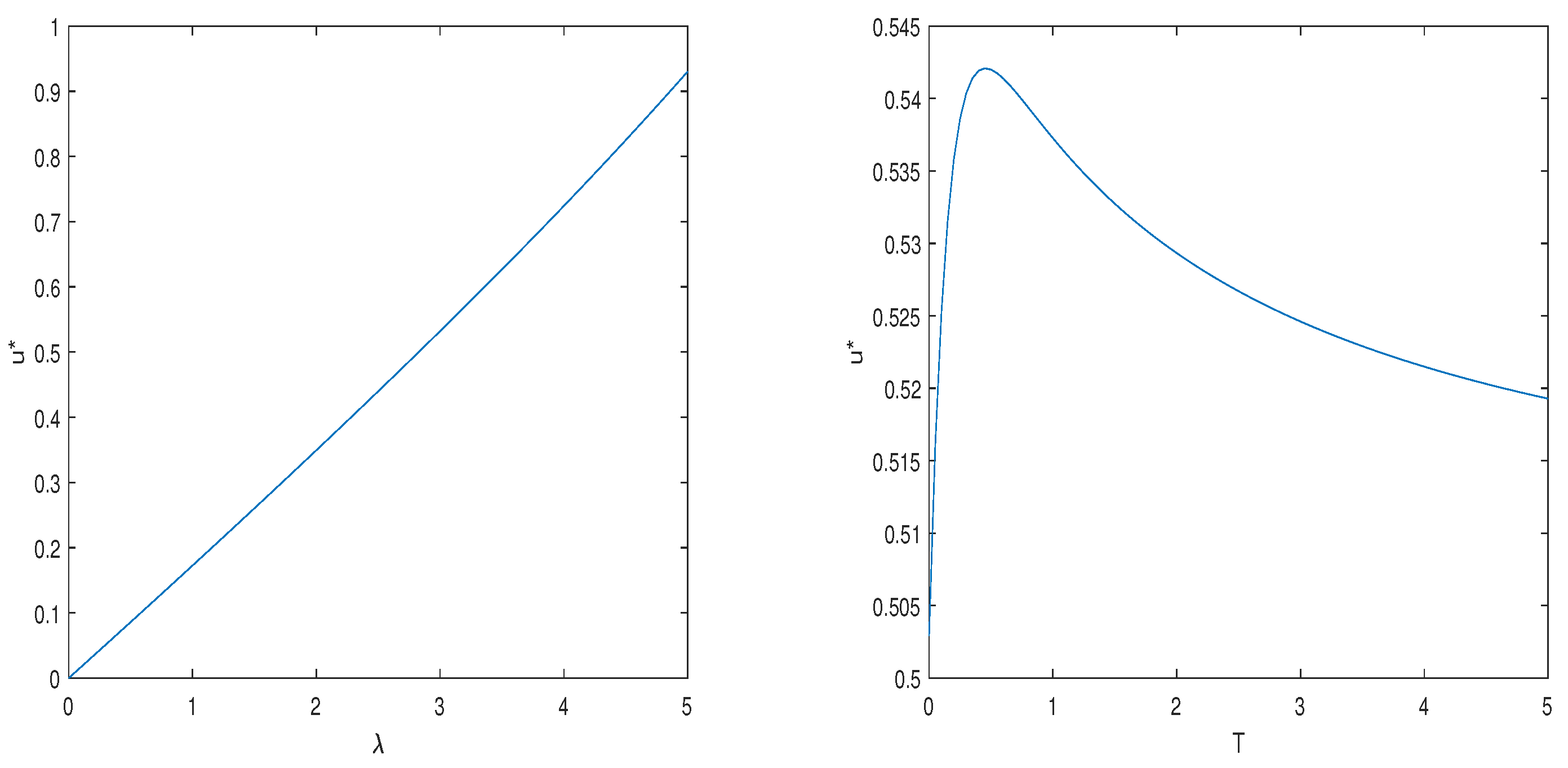
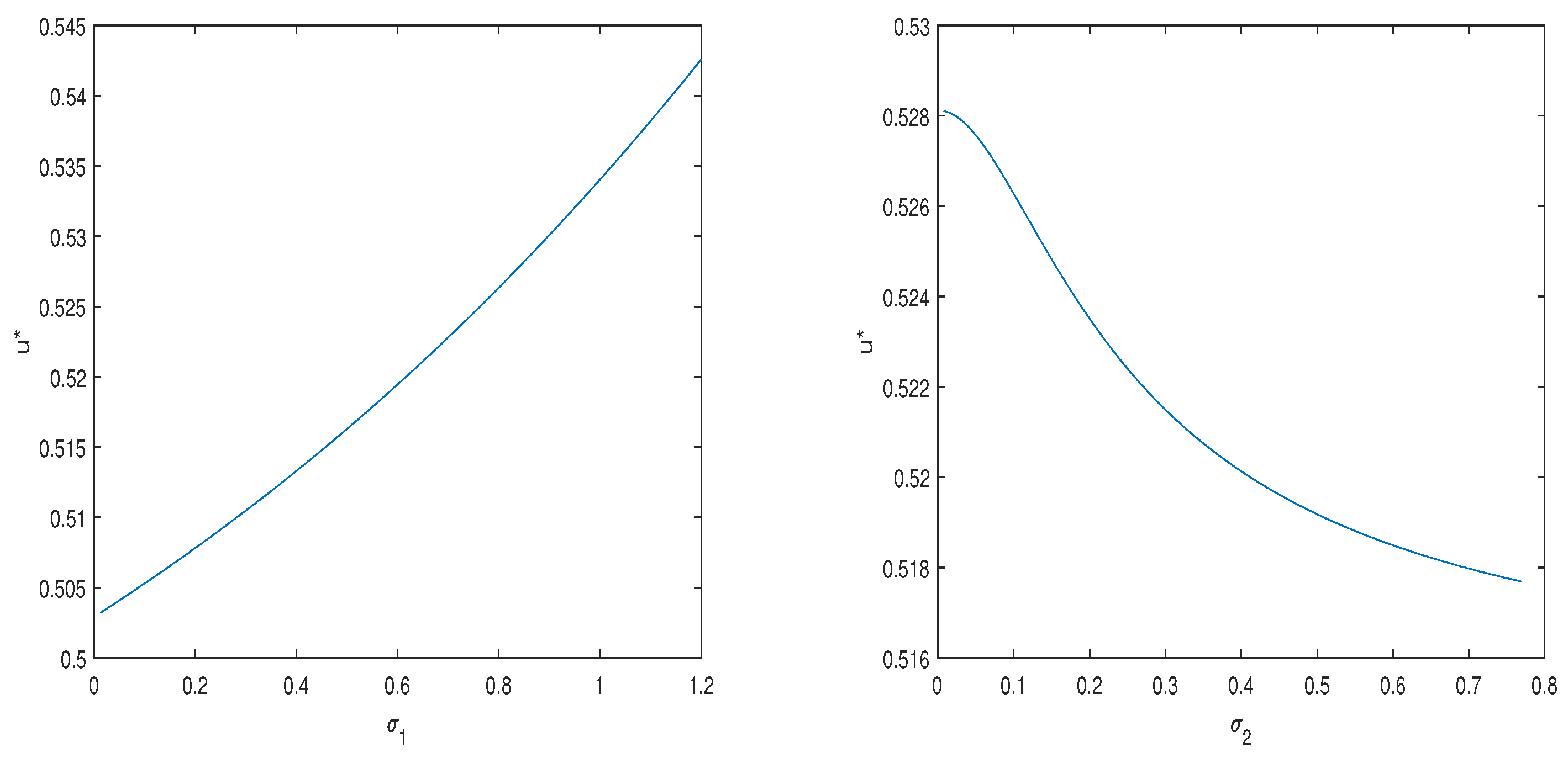
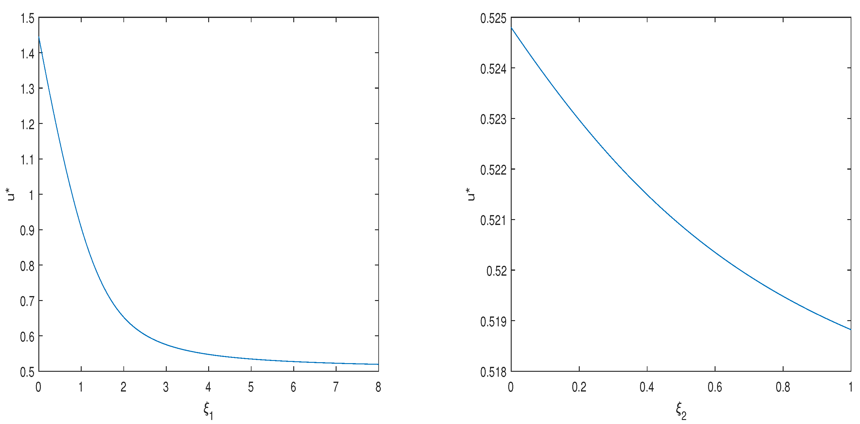
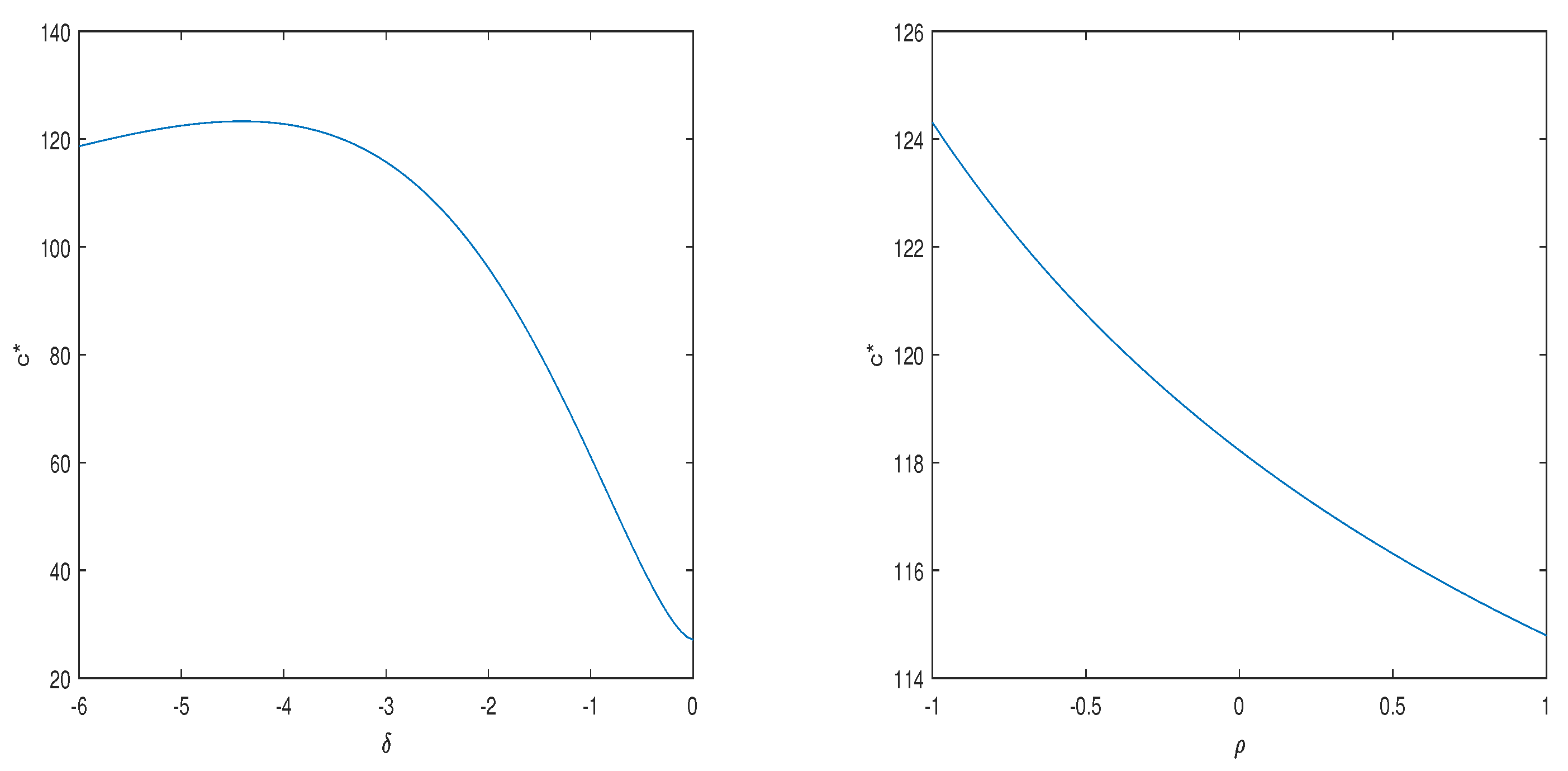
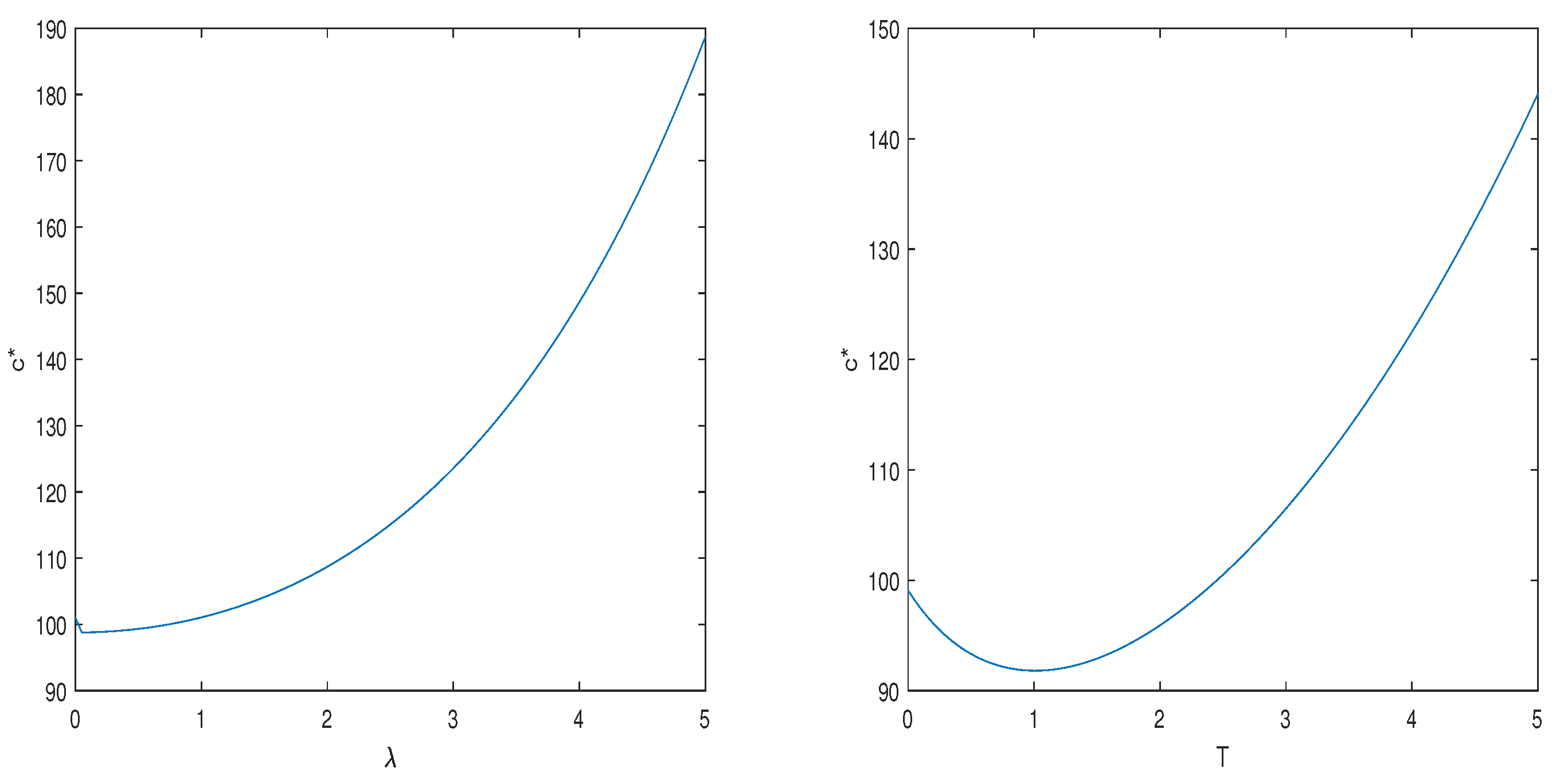
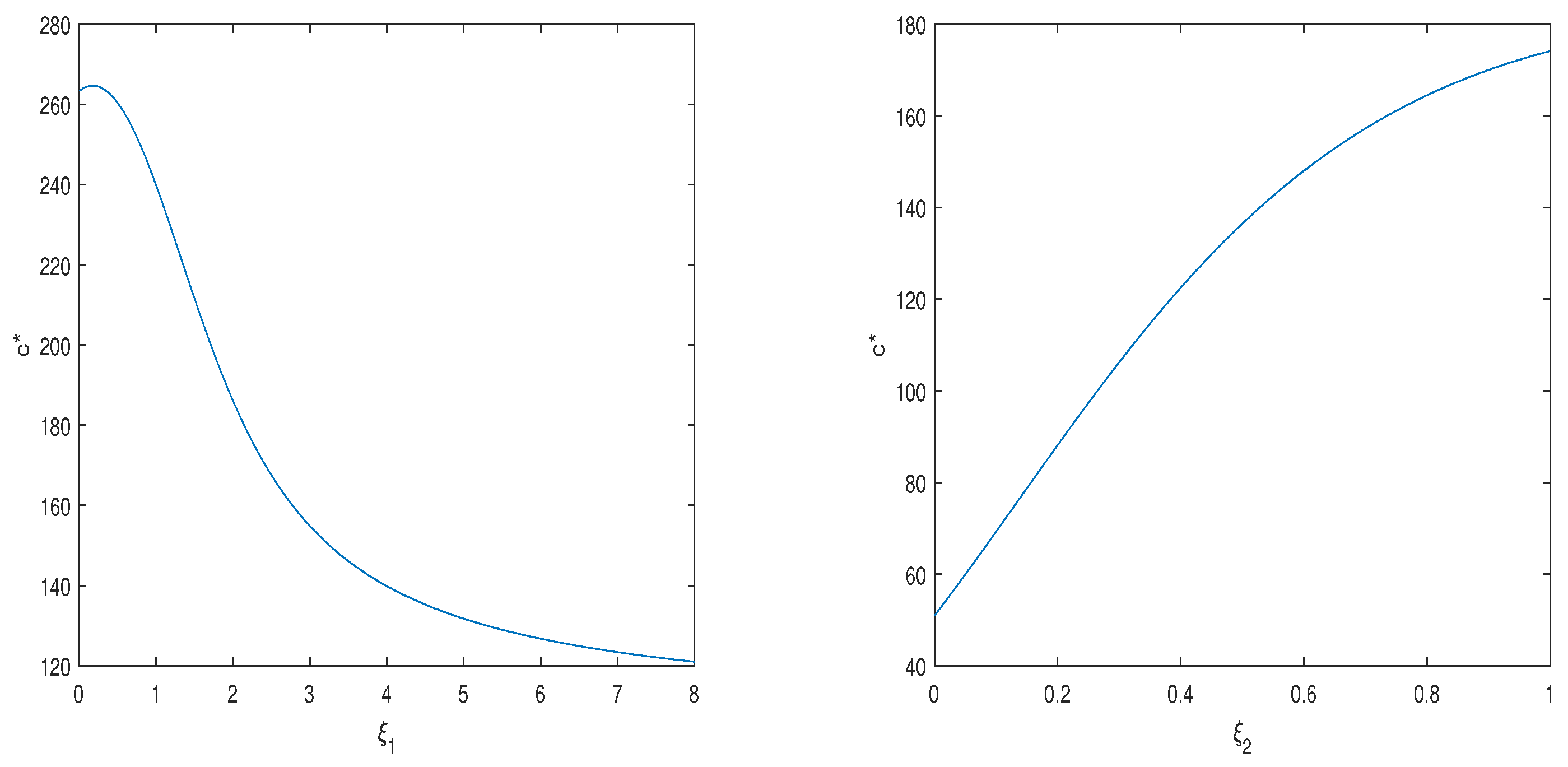
In the next section, numerical examples are given to verify the effect of the parameters in the 4/2-CIR stochastic hybrid model on the optimal consumption–investment strategy.

4. Numerical Example

In this section, we provide a numerical example to illustrate the effect of the model parameters in the 4/2-CIR stochastic hybrid model on the optimal consumption and investment strategies. Unless otherwise stated, we consider most of the model parameter settings adapted from Cheng et al. [21]: $a=0.9051,b=0.0023,t=0,T=4,{\sigma }_1=0.6612,{\xi }_1=7.3479,{\eta }_1=0.0328,\delta =-5,\lambda =2.9428,\rho =-0.7689$. Other parameters are given as follows: $v_0=0.0328,r_0=0.05,W_0=100,\beta =0.1,\alpha =0.4,{\sigma }_2=0.3,{\xi }_2=0.4,{\eta }_2=0.6$. The analysis was carried out with MATLAB software and the results are detailed in Figure 1, Figure 2, Figure 3, Figure 4, Figure 5, Figure 6, Figure 7 and Figure 8.

4.1. Impact on Optimal Investment Strategies

In this subsection, we study the influence of model parameters in the 4/2-CIR stochastic hybrid model on the optimal fraction of wealth invested in the risky asset. The relationships between the model parameters and the optimal investment strategy are shown in Figure 1, Figure 2, Figure 3 and Figure 4.

Figure 1 describes the relationship between the optimal fraction of wealth invested in risky assets $u^{*}$ and the coefficient of risk aversion $1-\delta$. It can be seen that the optimal investment strategy $u^{*}$ increases with the coefficient of risk aversion $1-\delta$. Intuitively, under the power utility function, the coefficient of risk aversion $1-\delta$ decreases as $\delta$ increases, that is, investors face less investment risk as $\delta$ increases. Therefore, the investor should increase their investment in risky assets. On the other hand, Figure 1 also presents the contribution of the correlation coefficient $\rho$ to the optimal fraction of wealth invested in risky assets. It can be seen that the optimal fraction of wealth invested in risky assets decreases with the increase in the correlation coefficient $\rho$. This conclusion is also obtained by Cheng et al. [21].

From Figure 2 we are able to obtain not only the influence of the excess return $\lambda$ on the optimal investment strategy $u^{*}$, but also the influence of the investment horizon T on the optimal investment strategy $u^{*}$. Specifically speaking, the optimal investment strategy increases as $\lambda$ increases. In fact, with the increase in $\lambda$, the excess return of risky assets becomes higher, and the investment wealth increases, so investors will increase the amount of investment in risky assets. Furthermore, the optimal fraction of wealth invested in risky assets first increases and then decreases with the increase in T. In the short term, investors are more willing to invest in risky assets, and the fraction of wealth invested in risky assets increases. In addition, the investment willingness will decrease as the investment period increases, so the optimal fraction of wealth invested in risky assets decreases.

From Figure 3, we can see the effect of the volatility of the volatility process ${\sigma }_1$ and the volatility of the interest rate ${\sigma }_2$ on the optimal investment strategy. At first, the optimal investment strategy $u^{*}$ increases with the increase in the volatility coefficient of volatility process ${\sigma }_1$. In the 4/2-CIR stochastic hybrid model, the factor influencing the investment share $\frac{v}{av+b}$ is a non-negative monotonic increasing function, when the volatility coefficient of the volatility process increases, the optimal fraction of wealth invested in risky assets will increase. This conclusion is consistent with Cheng et al. [21]. In addition, Figure 3 also shows the influence of the volatility coefficient of the interest rate on the optimal investment strategy. It can be seen that the optimal investment strategy increases with the increase in ${\sigma }_2$. As ${\sigma }_2$ increases, the risk of the interest rate becomes greater, so the investor will reduce savings and increase the fraction of wealth invested in risky assets.

We can obtain the influence of the mean-reverting speed of the volatility ${\xi }_1$ and the mean-reverting speed of the interest rate ${\xi }_2$ on the optimal investment strategy in Figure 4. At first, it shows that the optimal investment strategy decreases with the increase in ${\xi }_1$. As a matter of fact, with the increase in ${\xi }_1$, the expected volatility becomes smaller. Therefore, the expected stock appreciation rate becomes lower, and investors will reduce their investment in risky assets. In addition, the optimal investment strategy decreases with the increase in ${\xi }_2$. With the increase in ${\xi }_2$, the interest rate risk becomes smaller. Therefore, investors are more willing to increase savings and reduce investment in risky assets as ${\xi }_2$ increases.

4.2. Impact on Optimal Consumption Strategies

In this subsection, we analyze the influence of model parameters in the 4/2-CIR stochastic hybrid model on the optimal consumption strategy. The relationships between model parameters and the optimal consumption strategy are shown in Figure 5, Figure 6, Figure 7 and Figure 8.

Figure 5 illustrates the influence of the coefficient of risk aversion $1-\delta$ and correlation coefficient $\rho$ on the optimal consumption strategy $c^{*}$. It can be seen that the optimal consumption strategy decreases with the increase in the risk avoidance factor. Under the power effect function, the risk aversion level of investors becomes lower as $\delta$ increases. This means that they will increase the fraction of wealth invested in risky assets and reduce consumption. In addition, the optimal consumption strategy decreases with the increase in $\rho$ from Figure 5.

Figure 6 illustrates the impact of the excess return $\lambda$ and investment horizon T on optimal consumption. It can be seen that the optimal consumption strategy increases with the increase in excess return $\lambda$. The excess return increases with the increase in $\lambda$, that is, the investment wealth increases when $\lambda$ increases, so the optimal consumption strategy also increases. On the other hand, the optimal consumption strategy first decreases and then increases with the increase in T. In the short term, investors are more willing to invest in risky assets, which leads to the fact that the investor will reduce consumption. In addition, the investor will increase consumption as the investment period increases.

It can be seen from Figure 7 that the optimal consumption strategy increases with the increase in the volatility coefficient of the volatility process ${\sigma }_1$. This is mainly because with the increase in the volatility coefficient of the volatility process, the economic environment becomes more unstable, and investors are more willing to reduce investment and increase consumption. In addition, the relationship between the optimal consumption strategy and the volatility of the interest rate ${\sigma }_2$ can also be obtained from Figure 7. It can be seen that with the increase in the volatility of the interest rate ${\sigma }_2$, the risk of the interest rate will increase, so the investors will reduce savings and increase consumption.

Figure 8 illustrates the influence of the mean-reverting speed of volatility ${\xi }_1$ and the mean-reverting speed of the interest rate ${\xi }_2$ on the optimal consumption strategy. In fact, with the increase in ${\xi }_1$, investors’ willingness to consume decreases, and they will also spend less. In addition, the optimal consumption increases with the increase in the mean-reverting speed of the interest rate ${\xi }_2$. As ${\xi }_2$ increases, the interest rate fluctuation is smaller, and so investors will increase their savings and reduce consumption.

5. Conclusions

In this paper, we studied the problem of the optimal consumption and investment problem under the expected utility maximization criterion. The financial market consists of a risk-free asset and a risky asset. It is assumed that the price of risky assets follows the 4/2-CIR stochastic hybrid model. We found the solution of the optimal consumption and investment strategy under the power utility function. In the numerical example, we obtained the influence of model parameters on the optimal consumption–investment strategy.

We show the analytical representations of the optimal consumption–investment strategy, and value functions under the 4/2-CIR stochastic hybrid model by solving the SDEs. It is well known that changes in market interest rates and risky asset volatility affect the willingness of investors to invest, which has a significant impact on the optimal consumption–investment strategy. In our numerical example, we show that the optimal investment strategy increases with increases in $\lambda$ and ${\sigma }_1$, and decreases with increases in $\rho$, ${\sigma }_2$, ${\xi }_1$, and ${\xi }_2$. On the other hand, the optimal consumption strategy increases with increases in $\lambda$, ${\sigma }_1$, and ${\xi }_2$, and decreases with increases in $\rho$, ${\sigma }_2$, and ${\xi }_1$. In addition, the risk aversion factor $\delta$ and investment horizon T also have a significant impact on the optimal consumption–investment strategy.