On Some Classes of Harmonic Functions Associated with the Janowski Function

Abstract

In this paper, we introduce some classes of univalent harmonic functions with respect to the symmetric conjugate points by means of subordination, the analytic parts of which are reciprocal starlike (or convex) functions. Further, we discuss the geometric properties of the classes, such as the integral expression, coefficient estimation, distortion theorem, Jacobian estimation, growth estimates, and covering theorem.

1. Introduction

Define $\mathcal{A}$ as a class of analytic functions $\sigma$ of the form

$$\sigma \left(z\right)=z+{\displaystyle \sum _{k=2}^{\infty }}{\sigma }_k{z}^k,(z\in \mathbb{D}),$$

(1)

where $\mathbb{D}=\{z\in \mathbb{C}$ : $\left|z\right|<1\}$.

Let $\mathcal{S},{\mathcal{S}}^{*}$, and $\mathcal{K}$ be the subclasses of $\mathcal{A}$, which are composed of univalent functions, starlike functions, and convex functions, respectively [1,2].

Let $\mathcal{P}$ denote the class of analytic functions $p\left(z\right),\mathrm{Re}p\left(z\right)>0(z\in \mathbb{D})$ of the following form:

$$p\left(z\right)=1+{\displaystyle \sum _{j=1}^{\infty }}{p}_j{z}^j.$$

(2)

The function $p\in \mathcal{P}$ is called a Carathéodory function.

Suppose that the functions $\lambda$ and $\mu$ are analytic in $\mathbb{D}$. The function $\lambda$ is said to be subordinate to the function $\mu$ if there exists a function $\Theta$ satisfying $\Theta \left(0\right)=0\mathrm{and}|\Theta (z\left)\right|<1(z\in \mathbb{D})$, such that $\lambda \left(z\right)=\mu (\Theta (z\left)\right)(z\in \mathbb{D})$. Note that $\lambda \left(z\right)\prec \mu \left(z\right)$. In particular, if $\mu$ is univalent in $\mathbb{D}$, the following conclusion follows (see [1]):

$$\lambda \left(z\right)\prec \mu \left(z\right)⟺\lambda \left(0\right)=\mu \left(0\right)\mathrm{and}\lambda \left(\mathbb{D}\right)\subset \mu \left(\mathbb{D}\right).$$

In 1994, Ma and Minda [3] introduced the classes ${\mathcal{S}}^{*}\left(\vartheta \right)$ and $\mathcal{K}\left(\vartheta \right)$ of starlike functions and convex functions by using subordination. The function $\sigma \left(z\right)\in {\mathcal{S}}^{*}\left(\vartheta \right)$ iff $\frac{z{\sigma }^{\prime }\left(z\right)}{\sigma \left(z\right)}\prec \vartheta \left(z\right)$ and the function $\sigma \left(z\right)\in \mathcal{K}\left(\vartheta \right)$ iff $1+\frac{z{\sigma }^{″}\left(z\right)}{{\sigma }^{\prime }\left(z\right)}\prec \vartheta \left(z\right)$, where $\sigma \in \mathcal{A}$ and $\vartheta \in \mathcal{P}$.

Let $\vartheta \left(z\right)=\frac{1+az}{1+bz}$ and $-1\le b<a\le 1$. The classes ${\mathcal{S}}^{*}\left(\frac{1+az}{1+bz}\right)={\mathcal{S}}^{*}(a,b)$ and $\mathcal{K}\left(\frac{1+az}{1+bz}\right)=\mathcal{K}(a,b)$ are the classes of Janowski starlike and convex functions, respectively (refer to [4]). ${\mathcal{S}}^{*}\left(\frac{1+z}{1-z}\right)={\mathcal{S}}^{*}$ and $\mathcal{K}\left(\frac{1+z}{1-z}\right)=\mathcal{K}$ are known for the classes of starlike and convex functions, respectively.

In 1959, Sakaguchi [5] introduced the class ${\mathcal{S}}_s^{*}$ of starlike functions with respect to symmetric points. The function $\sigma \in {\mathcal{S}}_s^{*}$ if and only if

$$\mathrm{Re}\left(\frac{z{\sigma }^{\prime }\left(z\right)}{\sigma \left(z\right)-\sigma (-z)}\right)>0.$$

In 1987, El Ashwah and Thomas [6] introduced the classes ${\mathcal{S}}_c^{*}$ and ${\mathcal{S}}_{sc}^{*}$ of starlike functions with respect to conjugate points and symmetric conjugate points as follows:

$$\sigma \in {\mathcal{S}}_c^{*}⟺\mathrm{Re}\left(\frac{z{\sigma }^{\prime }\left(z\right)}{\sigma \left(z\right)+\overline{\sigma }\left(\overline{z}\right)}\right)>0\mathrm{and}\sigma \in {\mathcal{S}}_{sc}^{*}⟺\mathrm{Re}\left(\frac{z{\sigma }^{\prime }\left(z\right)}{\sigma \left(z\right)-\overline{\sigma }(-\overline{z})}\right)>0.$$

Similarly to the previous section, the classes ${\mathcal{S}}_c^{*}$ and ${\mathcal{S}}_{sc}^{*}$ can be further generalized to the classes ${\mathcal{S}}_{sc}^{*}\left(\vartheta \right)$ and ${\mathcal{K}}_{sc}\left(\vartheta \right)$.

The function $\sigma \left(z\right)$ belongs to ${\mathcal{S}}_{sc}^{*}\left(\vartheta \right)$ if and only if $\frac{2z{\sigma }^{\prime }\left(z\right)}{\sigma \left(z\right)-\overline{\sigma }(-\overline{z})}\prec \vartheta \left(z\right)$ holds true, and $\sigma \left(z\right)$ belongs to ${\mathcal{K}}_{sc}\left(\vartheta \right)$ if and only if $\frac{2{\left(z{\sigma }^{\prime }\left(z\right)\right)}^{\prime }}{{(\sigma \left(z\right)-\overline{\sigma }(-\overline{z}))}^{\prime }}\prec \vartheta \left(z\right)$ holds true, where $\sigma \in \mathcal{A}$ and $\vartheta \in \mathcal{P}$.

If the function $\sigma \in \mathcal{A}$ meets the following criteria—$\mathrm{Re}\left(\frac{\sigma \left(z\right)}{z{\sigma }^{\prime }\left(z\right)}\right)>\alpha (0\le \alpha <1)$—then $\sigma$ is said to be in the class of the reciprocal starlike functions of order $\alpha$, which is represented by $\sigma \in R{S}^{*}\left(\alpha \right)$.

In contrast to the classical starlike function class $S^{*}\left(\alpha \right)$ of order $\alpha$, the reciprocal starlike function class of order $\alpha$ maps the unit disk to a starlike region within a disk with $\left(\frac{1}{2\alpha },0\right)$ as the center and $\frac{1}{2\alpha }$ as the radius [7]. In particular, the disk is large when $0<\alpha <\frac{1}{2}$. Therefore, the study of the class of reciprocal starlike functions has aroused the research interest of most scholars [8,9,10,11,12,13]. In 2012, Sun et al. [8] extended the reciprocal starlike function to the class of the meromorphic univalent function.

As a generalization of the analytic function, the harmonic function has become one of the key branches in complex analysis because of the study of the minimal surface of parameters in differential geometry. After more than 20 years of development, harmonic function theory has been widely used in fluid dynamics, mathematical physics equations, and image processing, and it is also a powerful tool for studying minimal surfaces in differential geometry.

For the analytic functions $\sigma \left(z\right)$ and $\tau \left(z\right)(z\in \mathbb{D})$, let $S_H$ be a class of harmonic mappings that has the following form (see [14,15,16,17,18,19]):

$$f\left(z\right)=\sigma \left(z\right)+\overline{\tau \left(z\right)},z\in \mathbb{D},$$

(3)

where

$$\sigma \left(z\right)=z+{\displaystyle \sum _{k=2}^{\infty }}{\sigma }_k{z}^k\mathrm{and}\tau \left(z\right)={\displaystyle \sum _{k=1}^{\infty }}{\tau }_k{z}^k,\left|{\tau }_1\right|=\rho \in [0,1).$$

(4)

Specifically, $\sigma$ is referred to as the analytical part, and $\tau$ is known as the co-analytic part of f.

It is known that the function $f=\sigma \left(z\right)+\overline{\tau \left(z\right)}$ is locally univalent and sense-preserving in $\mathbb{D}$ if and only if $|{\sigma }^{\prime }\left(z\right)|>|{\tau }^{\prime }\left(z\right)|$ (see [20]).

Based on these results, it is possible to obtain the geometric properties of the co-analytic part by means of the analytic part of the harmonic function.

In the last few years, different subclasses of $S_H$ have been studied by several authors.

In 2007, Klimek and Michalski [21] investigated the subclass $S_H$ with $\sigma \in \mathcal{K}$.

In 2014, Hotta and Michalski [22] investigated the subclass $S_H$ with $\sigma \in \mathcal{S}$.

In 2015, Zhu and Huang [23] investigated the subclasses of $S_H$ with $\sigma \in {\mathcal{S}}^{*}\left(\frac{1+(1-2\beta )z}{1-z}\right)$ and $\sigma \in \mathcal{K}\left(\frac{1+(1-2\beta )z}{1-z}\right)$.

Combined with the above studies, by using the subordination relationship, this paper further constructs the reciprocal-structure harmonic function class with symmetric conjugate points as follows.

Definition 1.

Let $f=\sigma +\overline{\tau }$ be in the class $S_H$ of the Form (4) and let $-1\le b<a\le 1$. We define the class $HR{S}_{sc}^{*,\rho }(a,b)$ as that of univalent harmonic reciprocal starlike functions with a symmetric conjugate point; the function $f=\sigma +\overline{\tau }\in HR{S}_{sc}^{*,\rho }(a,b)$ if and only if $\sigma \in R{S}_{sc}^{*}(a,b)$, that is,

$$\frac{\sigma \left(z\right)-\overline{\sigma }(-\overline{z})}{2z{\sigma }^{\prime }\left(z\right)}\prec \frac{1+az}{1+bz}.$$

(5)

In addition, let $HR{K}_{sc}^{\rho }(a,b)$ define the class of harmonic univalent reciprocal convex functions with a symmetric conjugate point. The function $f=\sigma +\overline{\tau }\in HR{K}_{sc}^{\rho }(a,b)$ if and only if $\sigma \in R{K}_{sc}(a,b)$, that is,

$$\frac{{(\sigma \left(z\right)-\overline{\sigma }(-\overline{z}))}^{\prime }}{2{\left(z{\sigma }^{\prime }\left(z\right)\right)}^{\prime }}\prec \frac{1+az}{1+bz}.$$

(6)

In this paper, we discuss the geometric properties of these classes, such as the integral expression, coefficient estimation, distortion theorem, Jacobian estimation, growth estimate, and covering theorem. In order to show the geometric properties of the function more intuitively, we give the corresponding function image. The conclusion has enriched the field of research on harmonic functions.

2. Preliminary Preparation

To obtain our results, we need the following Lemmas.

Lemma 1

([24]). Let γ be a complex number. If the function $\Theta \left(z\right)$ is analytic in $\mathbb{D}$, satisfies $|\Theta (z\left)\right|\le 1$, and is of the form $\Theta \left(z\right)=c_0+c_{1}z+\cdots +c_n{z}^n+\cdots$, then

$$\left|c_n\right|\le 1-{\left|c_0\right|}^2,n=1,2,\cdots ,$$

and

$$\left|c_2-\gamma c_1^2\right|\le \max \{1,|\gamma \left|\right\}.$$

According to the subordination relationship, we get the integral expression of the classes $R{S}_{sc}^{*}(a,b)$ and $R{K}_{sc}^{*}(a,b)$ as follows.

Lemma 2.

Let $-1\le b<a\le 1$.

(1) 

If $\sigma \left(z\right)\in R{S}_{sc}^{*}(a,b),$ then

$$\sigma \left(z\right)={\int }_0^z\chi \left(\zeta \right)d\zeta ,$$

(7)

where

$$\chi \left(\zeta \right)=\frac{1+b\varpi \left(\zeta \right)}{1+a\varpi \left(\zeta \right)}\exp \left\{\frac{(b-a)}{2}{\int }_0^{\zeta }\frac{\varpi \left(t\right)}{t(1+a\varpi (t\left)\right)}+\frac{\overline{\varpi }(-\overline{t})}{t(1+a\overline{\varpi }(-\overline{t}))}dt\right\},$$

(8)

and ϖ is analytic in $\mathbb{D}$, satisfying $\varpi \left(0\right)=0,\left|\varpi \right(z\left)\right|<1$.

(2) 

If $\sigma \left(z\right)\in R{K}_{sc}^{*}(a,b),$ then

$$\sigma \left(z\right)={\int }_0^z\frac{1}{\xi }{\int }_0^{\xi }\chi \left(\zeta \right)d\zeta d\xi ,$$

where $\chi \left(\zeta \right)$ is given by (8) and ϖ is analytic in $\mathbb{D}$, satisfying $\varpi \left(0\right)=0,\left|\varpi \right(z\left)\right|<1$.

Proof. 

Let $\sigma \left(z\right)$ belong to the class $R{S}_{sc}^{*}(a,b)$. According to Definition 1 and the subordination principle, there exists an analytic function $\varpi$ in $\mathbb{D}$ that satisfies $\varpi \left(0\right)=0,\left|\varpi \right(z\left)\right|<1$ such that

$$\frac{\sigma \left(z\right)-\overline{\sigma }(-\overline{z})}{2z{\sigma }^{\prime }\left(z\right)}=\frac{1+a\varpi \left(z\right)}{1+b\varpi \left(z\right)}.$$

(9)

By replacing z in (9) with $-\overline{z}$, we get

$$\frac{\sigma (-\overline{z})-\overline{\sigma }\left(z\right)}{-2\overline{z}{\sigma }^{\prime }(-\overline{z})}=\frac{1+a\varpi (-\overline{z})}{1+b\varpi (-\overline{z})}.$$

(10)

By combining (9) and (10), the following formula can be established:

$$\frac{2z{(\overline{\sigma }\left(z\right)-\sigma (-\overline{z}))}^{\prime }}{\overline{\sigma }\left(z\right)-\sigma (-\overline{z})}=\frac{1+b\varpi \left(z\right)}{1+a\varpi \left(z\right)}+\frac{1+b\overline{\varpi }(-\overline{z})}{1+a\overline{\varpi }(-\overline{z})}.$$

(11)

We integrate both sides of Equation (11) and make a simple calculation to get the following result:

$$\frac{\overline{\sigma }\left(z\right)-\sigma (-\overline{z})}{2}=z\exp \left\{\frac{(b-a)}{2}{\int }_0^z\frac{\varpi \left(t\right)}{t(1+a\varpi (t\left)\right)}+\frac{\overline{\varpi }(-\overline{t})}{t(1+a\overline{\varpi }(-\overline{t}))}dt\right\}.$$

(12)

From (9) and (12), we have

$${\sigma }^{\prime }\left(z\right)=\frac{1+b\varpi \left(z\right)}{1+a\varpi \left(z\right)}\exp \left\{\frac{(b-a)}{2}{\int }_0^z\frac{\varpi \left(t\right)}{t(1+a\varpi (t\left)\right)}+\frac{\overline{\varpi }(-\overline{t})}{t(1+a\overline{\varpi }(-\overline{t}))}dt\right\}.$$

(13)

We integrate both sides of Equation (13) again, and we get

$$\sigma \left(z\right)={\int }_0^z\frac{1+b\varpi \left(\zeta \right)}{1+a\varpi \left(\zeta \right)}\exp \left\{\frac{(b-a)}{2}{\int }_0^{\zeta }\frac{\varpi \left(t\right)}{t(1+a\varpi (t\left)\right)}+\frac{\overline{\varpi }(-\overline{t})}{t(1+a\overline{\varpi }(-\overline{t}))}dt\right\}d\zeta .$$

According to (7), we have $\sigma \in R{K}_{sc}(a,b)$ if and only if $z{\sigma }^{\prime }\left(z\right)\in R{S}_{sc}^{*}(a,b)$. So, we can easily get (8).     □

Lemma 3.

Let $-1\le b<a\le 1$ and $\sigma \left(z\right)=z+{\displaystyle \sum _{k=2}^{\infty }}{\sigma }_k{z}^k$.

(1) 

If $\sigma \left(z\right)\in R{S}_{sc}^{*}(a,b),$ then

$$|{\sigma }_{2n}|\le \frac{(a-b)}{2n}{G}_{n-1}(a,b),$$

(14)

and

$$|{\sigma }_{2n+1}|\le \frac{(a-b)(1+a-b)}{2n}{G}_{n-1}(a,b).$$

(15)

In particular, $|{\sigma }_2|\le \frac{a-b}{2}$ and $|{\sigma }_3|\le \frac{(a-b)}{2}(1+a-b)$.

The estimate is sharp if

$$\sigma \left(z\right)={\int }_0^z\frac{(1-\xi ){[1-{(1+a-b)}^2{\xi }^2]}^{-\frac{(a-b)}{2(1+a-b)}}}{1-(1+a-b)\xi }d\xi .$$

(2) 

If $\sigma \left(z\right)\in R{K}_{sc}(a,b),$ then

$$|{\sigma }_{2n}|\le \frac{(a-b)}{4n^2}{G}_{n-1}(a,b),$$

(16)

and

$$|{\sigma }_{2n+1}|\le \frac{(a-b)(1+a-b)}{2n(2n+1)}{G}_{n-1}(a,b),$$

(17)

where

$$G_m(a,b)={(1+a-b)}^m{\displaystyle \prod _{k=1}^m}\left(1+\frac{(2k+1)(a-b)}{2k}\right),m\ge 1.$$

(18)

In particular, $|{\sigma }_2|\le \frac{a-b}{4}$ and $|{\sigma }_3|\le \frac{(a-b)}{6}(1+a-b)$.

The estimate is sharp if

$$\sigma \left(z\right)={\int }_0^z\frac{1}{\eta }{\int }_0^{\eta }\frac{(1-\xi ){[1-{(1+a-b)}^2{\xi }^2]}^{-\frac{(a-b)}{2(1+a-b)}}}{1-(1+a-b)\xi }d\xi d\eta .$$

In particular, if $a=1$ and $b=-1$, we get the following conclusion.

(1) 

If $\sigma \left(z\right)\in R{S}_{sc}^{*},$ then

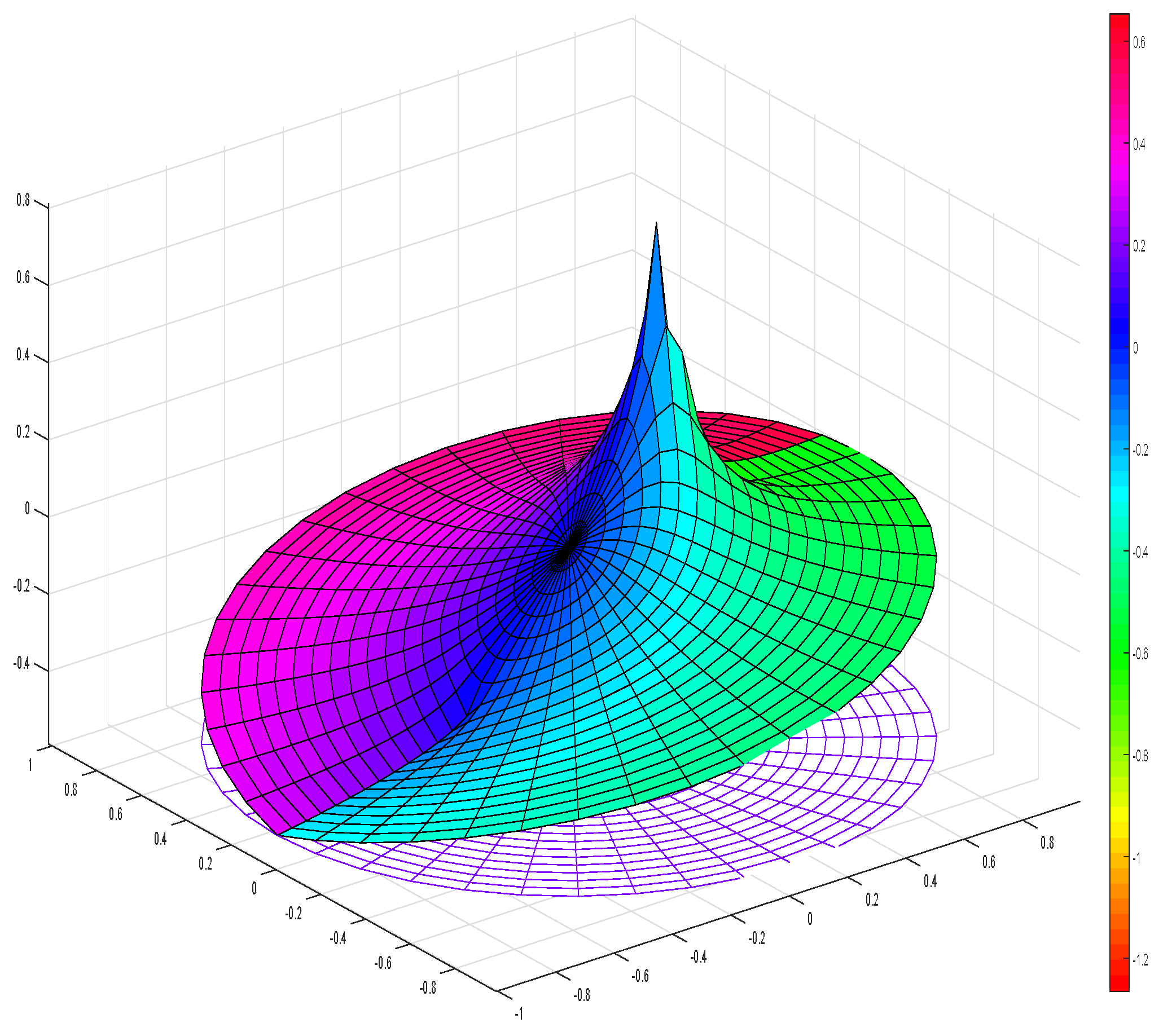
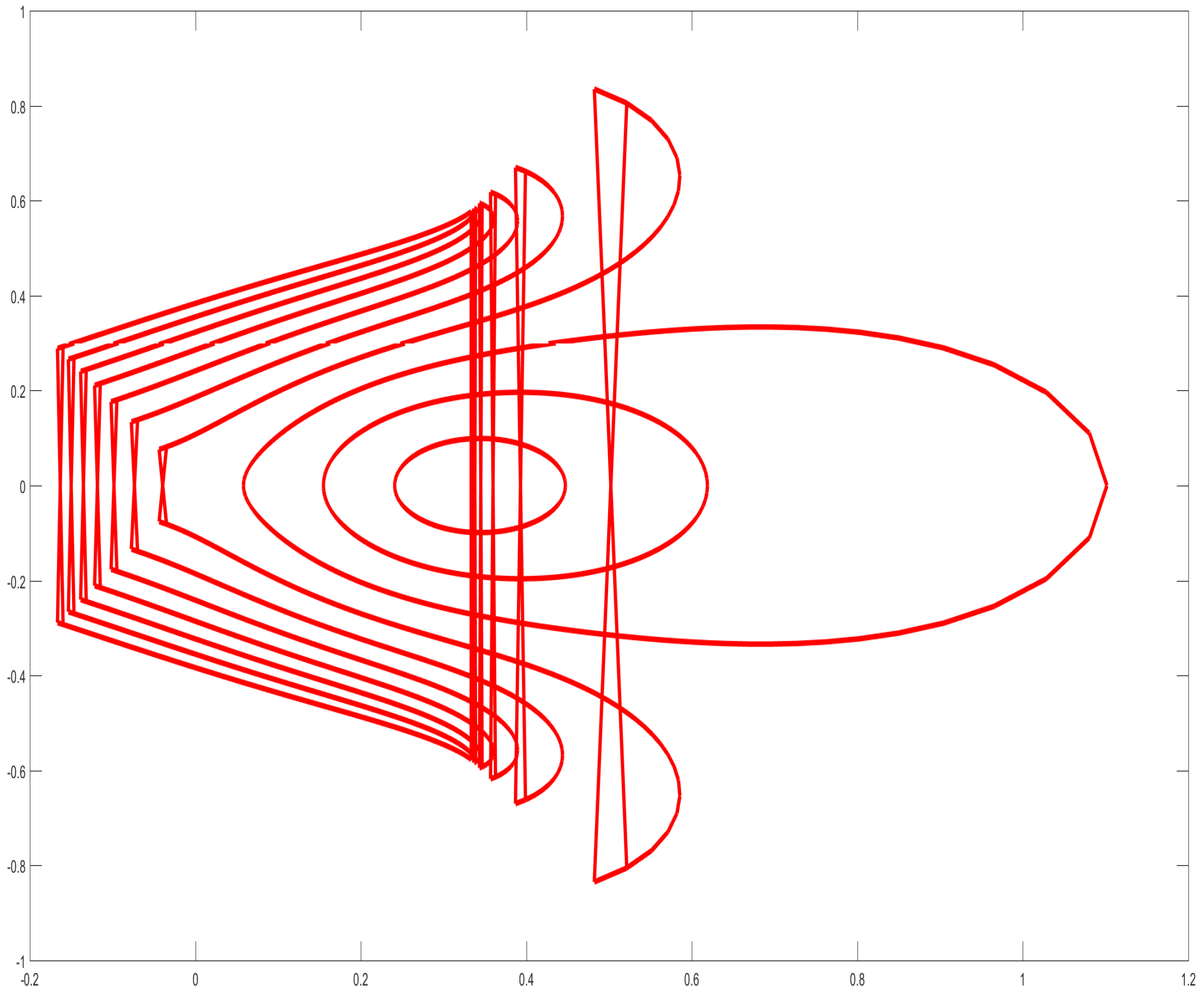
$$|{\sigma }_{2n}|\le \frac{3^{n-1}}{n!}{\displaystyle \prod _{k=1}^{n-1}}(3k+1)\mathit{and}|{\sigma }_{2n+1}|\le \frac{3^n}{n!}{\displaystyle \prod _{k=1}^{n-1}}(3k+1).$$

The estimate is sharp if $\sigma \left(z\right)=\frac{{(1+3z)}^{\frac{2}{3}}}{3{(1-3z)}^{\frac{1}{3}}}-\frac{1}{3}$, and a graph of this function is shown in Figure 1. In the figure, the complex function $\sigma \left(z\right)$ is represented by the three-dimensional coordinate system plus color; the $x$-axis represents the real part of the variable z; the $y$-axis represents the imaginary part of the variable z; the $z$-axis represents the real part of the function $\sigma \left(z\right)$, and the color represents the imaginary part of the function $\sigma \left(z\right)$. In Figure 2, the range of the function $\sigma \left(z\right)$ is shown, with the $x$-axis representing the real part of the function $\sigma \left(z\right)$ and the $y$-axis representing the imaginary part of the function $\sigma \left(z\right)$.

(2) 

If $\sigma \left(z\right)\in R{K}_{sc},$ then

$$|{\sigma }_{2n}|\le \frac{3^{n-1}}{\left(2n\right)n!}{\displaystyle \prod _{k=1}^{n-1}}(3k+1)\mathit{and}|{\sigma }_{2n+1}|\le \frac{3^n}{(2n+1)n!}{\displaystyle \prod _{k=1}^{n-1}}(3k+1).$$

The estimate is sharp if

$$\sigma \left(z\right)={\int }_0^z\frac{{(1+3\eta )}^{\frac{2}{3}}}{3\eta {(1-3\eta )}^{\frac{1}{3}}}-\frac{1}{3\eta }d\eta .$$

Proof. 

First, we prove the first part of Lemma 3. Let $\sigma \left(z\right)=z+{\displaystyle \sum _{k=2}^{\infty }}{\sigma }_k{z}^k\in R{S}_{sc}^{*}(a,b)$, and there exists a positive real function $p\left(z\right)=1+{\displaystyle \sum _{j=1}^{\infty }}{p}_j{z}^j\in \mathcal{P}$ with $|p_j|\le a-b$ that satisfies the following condition:

$$\frac{\sigma \left(z\right)-\overline{\sigma }(-\overline{z})}{2z{\sigma }^{\prime }\left(z\right)}=p\left(z\right).$$

By comparing the coefficients of the two sides of the equation, the following conclusions are drawn:

$$2n{\sigma }_{2n}=-p_{2n-1}-2{\sigma }_2{p}_{2n-2}-3{\sigma }_3{p}_{2n-3}-\cdots -(2n-1){\sigma }_{2n-1}{p}_1,$$

and

$$2n{\sigma }_{2n+1}=-p_{2n}-2{\sigma }_2{p}_{2n-1}-3{\sigma }_3{p}_{2n-2}-\cdots -2n{\sigma }_{2n}{p}_1.$$

It is easy to prove that

$$|{\sigma }_{2n}|\le \frac{(a-b)}{2n}(1+2|{\sigma }_2|+\cdots +(2n-1)|{\sigma }_{2n-1}\left|\right),$$

(19)

and

$$|{\sigma }_{2n+1}|\le \frac{(a-b)}{2n}(1+2|{\sigma }_2|+\cdots +2n|{\sigma }_{2n}\left|\right).$$

(20)

From (19) and (20), we have

$$1+2|{\sigma }_2|+\cdots +(2n+1)|{\sigma }_{2n+1}{|\le (1+a-b)}^n{\displaystyle \prod _{k=1}^n}\left(1+\frac{(2k+1)}{2k}(a-b)\right),$$

(21)

and

$$1+2|{\sigma }_2|+\cdots +\left(2n\right)|{\sigma }_{2n}{|\le (1+a-b)}^n{\displaystyle \prod _{k=1}^{n-1}}\left(1+\frac{(2k+1)}{2k}(a-b)\right).$$

(22)

According to (19)–(22), we can obtain (14) and (15), that is,

$$|{\sigma }_{2n}|\le \frac{(a-b)}{2n}{(1+a-b)}^{n-1}{\displaystyle \prod _{k=1}^{n-1}}\left(1+\frac{(2k+1)(a-b)}{2k}\right)$$

and

$$|{\sigma }_{2n+1}|\le \frac{(a-b)}{2n}{(1+a-b)}^n{\displaystyle \prod _{k=1}^{n-1}}\left(1+\frac{(2k+1)(a-b)}{2k}\right).$$

The second part of Lemma 3 is shown below. Let $\sigma \left(z\right)=z+{\displaystyle \sum _{k=2}^{\infty }}{\sigma }_k{z}^k\in K_{sc}(a,b)$. Similarly to the previous proof, we can obtain

$$\frac{{(\sigma \left(z\right)-\overline{\sigma }(-\overline{z}))}^{\prime }}{2{\left(z{\sigma }^{\prime }\left(z\right)\right)}^{\prime }}=p\left(z\right),$$

where $p\left(z\right)=1+{\displaystyle \sum _{j=1}^{\infty }}{p}_j{z}^j\in \mathcal{P}$ is a positive real function with $|p_j|\le a-b$.

By comparing the coefficients of the two sides of the equation, we can get the following results:

$$\begin{array}{cc}\hfill 2^2{\sigma }_2& =-p_1,\hfill \\ \hfill 3·2{\sigma }_3& =-p_2-2^2{\sigma }_2{p}_1,\hfill \\ \hfill 4^2{\sigma }_4& =-p_3-2^2{\sigma }_2{p}_2-3^2{\sigma }_3{p}_1,\hfill \\ \hfill 5·4{\sigma }_5& =-p_4-2^2{\sigma }_2{p}_3-3^2{\sigma }_3{p}_2-2^2{\sigma }_2{p}_1,\hfill \\ \hfill & ⋮\hfill \\ \hfill {\left(2n\right)}^2{\sigma }_{2n}& =-p_{2n-1}-2^2{\sigma }_2{p}_{2n-2}-3^2{\sigma }_3{p}_{2n-3}-\cdots -{(2n-1)}^2{\sigma }_{2n-1}{p}_1,\hfill \\ \hfill (2n+1)\left(2n\right){\sigma }_{2n+1}& =-p_{2n}-2^2{\sigma }_2{p}_{2n-1}-3^2{\sigma }_3{p}_{2n-2}-\cdots -{\left(2n\right)}^2{\sigma }_{2n}{p}_1.\hfill \end{array}$$

It is easy to see that

$$|{\sigma }_{2n}|\le \frac{(a-b)}{{\left(2n\right)}^2}(1+2^2|{\sigma }_2{|+\cdots +(2n-1)}^2|{\sigma }_{2n-1}|),$$

(23)

and

$$|{\sigma }_{2n+1}|\le \frac{(a-b)}{2n(2n+1)}(1+2^2|{\sigma }_2{|+\cdots +\left(2n\right)}^2|{\sigma }_{2n}|).$$

(24)

From (23) and (24), we have

$$1+2^2|{\sigma }_2{|+\cdots +\left(2n\right)}^2|{\sigma }_{2n}|\le {(1+a-b)}^n{\displaystyle \prod _{k=1}^{n-1}}\left(1+\frac{(2k+1)}{2k}(a-b)\right),$$

(25)

and

$$1+2^2|{\sigma }_2{|+\cdots +(2n+1)}^2|{\sigma }_{2n+1}|\le {(1+a-b)}^n{\displaystyle \prod _{k=1}^n}\left(1+\frac{(2k+1)}{2k}(a-b)\right)$$

(26)

According to (23)–(26), we can obtain (16) and (17), that is,

$$|{\sigma }_{2n}|\le \frac{(a-b)}{{\left(2n\right)}^2}{(1+a-b)}^{n-1}{\displaystyle \prod _{k=1}^{n-1}}\left(1+\frac{(2k+1)}{2k}(a-b)\right),$$

and

$$|{\sigma }_{2n+1}|\le \frac{(a-b)}{\left(2n\right)(2n+1)}{(1+a-b)}^n{\displaystyle \prod _{k=1}^{n-1}}\left(1+\frac{(2k+1)}{2k}(a-b)\right).$$

□

Lemma 4.

Let $-1\le b<a\le 1,\mu \in \mathbb{C}$.

(1) 

If $\sigma \left(z\right)=z+{\displaystyle {\sum }_{k=2}^{\infty }}{\sigma }_k{z}^k\in R{S}_{sc}^{*}(a,b)$, then

$$\left|{\sigma }_3-\mu {\sigma }_2^2\right|\le \frac{a-b}{2}\max \left\{1,\left|a+\frac{\mu }{2}(b-a)\right|\right\}.$$

(27)

The estimate is sharp if

$$\sigma \left(z\right)={\int }_0^z(1+b\xi ){(1-a\xi )}^{\frac{b-a}{2a}}{(1+a\xi )}^{\frac{b-3a}{2a}}d\xi ,$$

or

$$\sigma \left(z\right)={\int }_0^z\left(1+b{\xi }^2\right){\left(1+a{\xi }^2\right)}^{\frac{b-3a}{2a}}d\xi .$$

(2) 

If $\sigma \left(z\right)=z+{\displaystyle {\sum }_{k=2}^{\infty }}{\sigma }_k{z}^k\in R{K}_{sc}(a,b)$, then

$$\left|{\sigma }_3-\mu {\sigma }_2^2\right|\le \frac{a-b}{6}\max \left\{1,\left|a+\frac{3\mu (b-a)}{8}\right|\right\}.$$

(28)

The estimate is sharp if

$$\sigma \left(z\right)={\int }_0^z\frac{1}{\eta }{\int }_0^{\eta }(1+b\xi ){(1-a\xi )}^{\frac{b-a}{2a}}{(1+a\xi )}^{\frac{b-3a}{2a}}d\xi d\eta ,$$

or

$$\sigma \left(z\right)={\int }_0^z\frac{1}{\eta }{\int }_0^{\eta }\left(1+b{\xi }^2\right){\left(1+a{\xi }^2\right)}^{\frac{b-3a}{2a}}d\xi d\eta .$$

In particular, if $a=1,b=-1$, we have the following results:

(1) 

If $\sigma \left(z\right)=z+{\displaystyle {\sum }_{k=2}^{\infty }}{\sigma }_k{z}^k\in R{S}_{sc}^{*}$, then

$$\left|{\sigma }_3-\mu {\sigma }_2^2\right|\le \max \left\{1,\left|1-\mu \right|\right\}.$$

The estimate is sharp if $\sigma \left(z\right)=\frac{z}{1+z}$ or $\sigma \left(z\right)=\frac{z}{1+z^2}$.

(2) 

If $\sigma \left(z\right)=z+{\displaystyle {\sum }_{k=2}^{\infty }}{\sigma }_k{z}^k\in R{K}_{sc}$, then

$$\left|{\sigma }_3-\mu {\sigma }_2^2\right|\le \frac{1}{3}\max \{1,|1-\frac{3\mu }{4}\left|\right\}.$$

The estimate is sharp if $\sigma \left(z\right)=\log (1+z)$ or $\sigma \left(z\right)=arctanz$.

Proof. 

Let $\sigma \left(z\right)=z+{\displaystyle {\sum }_{k=2}^{\infty }}{\sigma }_k{z}^k\in R{S}_{sc}^{*}(a,b)$. According to Definition 1 and the subordination principle, there exists an analytic function $\varpi \left(z\right)=c_{1}z+c_2{z}^2+\cdots$ in $\mathbb{D}$ that satisfies $\varpi \left(0\right)=0,\left|\varpi \right(z\left)\right|<1$ such that

$$\frac{\sigma \left(z\right)-\overline{\sigma }(-\overline{z})}{2z{\sigma }^{\prime }\left(z\right)}=\frac{1+a\varpi \left(z\right)}{1+b\varpi \left(z\right)}.$$

(29)

By comparing the coefficients of the two sides of Equation (29), we get the following results:

$${\sigma }_2=\frac{b-a}{2}{c}_1\mathrm{and}{a}_3=\frac{b-a}{2}{c}_2-\frac{(b-a)a}{2}{c}_1^2.$$

Therefore, we have

$${\sigma }_3-\mu {\sigma }_2^2=\frac{b-a}{2}\left\{c_2-\left(a+\frac{\mu (b-a)}{2}\right)c_1^2\right\}.$$

Applying Lemma 1, we get (27). The extremal function is as follows:

$$\sigma \left(z\right)={\int }_0^z(1+b\xi ){(1-a\xi )}^{\frac{b-a}{2A}}{(1+a\xi )}^{\frac{b-3a}{2a}}d\xi ,$$

or

$$\sigma \left(z\right)={\int }_0^z\left(1+b{\xi }^2\right){\left(1+a{\xi }^2\right)}^{\frac{b-3a}{2a}}d\xi .$$

If $\sigma \left(z\right)=z+{\displaystyle {\sum }_{k=2}^{\infty }}{\sigma }_k{z}^k\in R{K}_{sc}(a,b)$, then $z{\sigma }^{\prime }\left(z\right)\in R{S}_{sc}^{*}(a,b)$. It is easy to obtain (28), and the bound is sharp, as shown in the following:

$$\sigma \left(z\right)={\int }_0^z\frac{1}{\eta }{\int }_0^{\eta }(1+b\xi ){(1-a\xi )}^{\frac{b-a}{2a}}{(1+a\xi )}^{\frac{b-3a}{2a}}d\xi d\eta ,$$

or

$$\sigma \left(z\right)={\int }_0^z\frac{1}{\eta }{\int }_0^{\eta }\left(1+b{\xi }^2\right){\left(1+a{\xi }^2\right)}^{\frac{b-3a}{2a}}d\xi d\eta .$$

□

Lemma 5.

Let $-1\le b<a\le 1$ and $\left|z\right|=r\in [0,1)$.

(1) 

If $\sigma \left(z\right)\in R{S}^{*}(a,b)$, then

$$m_1(r;a,b)\le \left|\sigma \left(z\right)\right|\le M_1(r;a,b),$$

(30)

and

$$m_2(r;a,b)\le \left|{\sigma }^{\prime }\left(z\right)\right|\le M_2(r;a,b).$$

(31)

(2) 

If $\sigma \left(z\right)\in RK(a,b)$, then

$$m_3(r;a,b)\le \left|\sigma \left(z\right)\right|\le M_3(r;a,b),$$

(32)

and

$$\frac{m_1(r;a,b)}{r}\le \left|{\sigma }^{\prime }\left(z\right)\right|\le \frac{M_1(r;a,b)}{r},$$

(33)

where

$$M_1(r;a,b)=\left\{\begin{array}{cc}r{(1-ar)}^{\frac{b-a}{a}},& a\ne 0,\\ r{e}^{-br},& a=0,\end{array}\right.$$

(34)

$$m_1(r;a,b)=\left\{\begin{array}{cc}r{(1+ar)}^{\frac{b-a}{a}},& a\ne 0,\\ r{e}^{br},& a=0,\end{array}\right.$$

(35)

$$M_2(r;a,b)=\left\{\begin{array}{cc}{(1-ar)}^{\frac{b-2a}{a}}(1-br),& a\ne 0,\\ (1-br)e^{-br},& a=0,\end{array}\right.$$

(36)

$$m_2(r;a,b)=\left\{\begin{array}{cc}{(1+ar)}^{\frac{b-2a}{a}}(1+br),& a\ne 0,\\ (1+br)e^{br},& a=0,\end{array}\right.$$

(37)

$$M_3(r;a,b)=\left\{\begin{array}{cc}\frac{1}{b}-\frac{1}{b}{(1-ar)}^{\frac{b}{a}},& a\ne 0,\\ \frac{1}{b}-\frac{1}{b}{e}^{-br},& a=0,\end{array}\right.$$

(38)

$$m_3(r;a,b)=\left\{\begin{array}{cc}\frac{1}{b}{(1+ar)}^{\frac{b}{a}}-\frac{1}{b},& a\ne 0,\\ \frac{1}{b}{e}^{br}-\frac{1}{b},& a=0.\end{array}\right.$$

(39)

Proof. 

For $\sigma \left(z\right)\in R{S}^{*}(a,b)$, we let

$$\frac{\sigma \left(z\right)}{z{\sigma }^{\prime }\left(z\right)}=P\left(z\right)\mathrm{and}P\left(z\right)\prec \frac{1+az}{1+bz}.$$

After a simple calculation, we can get

$$\sigma \left(z\right)=z·\exp \left[\left({\int }_0^z\frac{1-P\left(\zeta \right)}{\zeta P\left(\zeta \right)}d\zeta \right)\right].$$

Therefore,

$$|\frac{\sigma \left(z\right)}{z}|=\exp \left(\mathrm{Re}{\int }_0^z\frac{1-P\left(\zeta \right)}{\zeta P\left(\zeta \right)}d\zeta \right).$$

Substituting $\zeta =zt$, we obtain

$$|\sigma \left(z\right)|=|z|exp\left({\int }_0^1\mathrm{Re}\frac{1-P\left(zt\right)}{tP\left(zt\right)}dt\right).$$

(40)

Letting $z=x+iy$ and $\left|z\right|=r\in (0,1]$, we get

$$\mathrm{Re}\frac{(b-a)z}{1+azt}dt=\frac{(b-a)(x+a{r}^{2}t)}{1+a^2{r}^2{t}^2+2axt}:=\Theta \left(x\right).$$

It is easy to find that $\Theta \left(x\right)$ is decreasing with respect to $x\in [-r,r]$. Therefore,

$$-\frac{(a-b)r}{1+art}\le \mathrm{Re}\frac{(b-a)z}{1+azt}\le \frac{(a-b)r}{1-art},$$

that is,

$$-\frac{(a-b)r}{1+art}\le \mathrm{Re}\frac{1-P\left(zt\right)}{tP\left(zt\right)}\le \frac{(a-b)r}{1-art}.$$

Integrating the two sides of the inequality for t above from 0 to 1, we get

$${(1+ar)}^{\frac{b-a}{a}}\le \exp {\int }_0^1\mathrm{Re}\frac{1-P\left(zt\right)}{tP\left(zt\right)}dt\le {(1-ar)}^{\frac{b-a}{a}},(a\ne 0),$$

(41)

and

$$e^{br}\le \exp {\int }_0^1\mathrm{Re}\frac{1-P\left(zt\right)}{tP\left(zt\right)}dt\le e^{-br},(a=0).$$

(42)

By combining inequalities (40)–(42), we can obtain (30) from Lemma 5.

On the other hand, for $\left|z\right|=r$, we have

$$\frac{1-ar}{1-br}<\left|\frac{\sigma \left(z\right)}{z{\sigma }^{\prime }\left(z\right)}\right|<\frac{1+ar}{1+br}.$$

(43)

From (41)–(43), we can obtain (31) from Lemma 5.

If $\sigma \left(z\right)\in RK(a,b)$, then $z{\sigma }^{\prime }\left(z\right)\in R{S}^{*}(a,b)$. According to the results in (30), we can easily get (33), that is,

$$\frac{m_1(r;a,b)}{r}\le \left|{\sigma }^{\prime }\left(z\right)\right|\le \frac{M_1(r;a,b)}{r},$$

By integrating the two sides of the inequality from 0 to r, we can get (32).     □

Lemma 6.

If $\sigma \left(z\right)\in {RS}_{sc}^{*}(a,b)$, then $\frac{\sigma \left(z\right)-\overline{\sigma }(-\overline{z})}{2}\in {RS}^{*}(a,b)$.

Proof. 

For convenience, we set $\Delta \sigma \left(z\right)=\frac{\sigma \left(z\right)-\overline{\sigma }(-\overline{z})}{2}$ and $D\sigma \left(z\right)=z{\sigma }^{\prime }\left(z\right)$.

Let $\sigma \left(z\right)\in {RS}_{sc}^{*}(a,b)$. According to Definition 1 and the relationship of subordination, we have

$$\frac{\sigma \left(z\right)-\overline{\sigma }(-\overline{z})}{2z{\sigma }^{\prime }\left(z\right)}=\frac{1+av\left(z\right)}{1+bv\left(z\right)},$$

that is,

$$\frac{\Delta \sigma \left(z\right)}{D\sigma \left(z\right)}=\frac{1+av\left(z\right)}{1+bv\left(z\right)},$$

where $v\left(z\right)$ is analytic in $\mathbb{U}$ and satisfies $v\left(0\right)=0$ and $\left|v\right(z\left)\right|<1$.

Let $p\left(z\right)=\frac{1+v\left(z\right)}{1+v\left(z\right)}$, and we have $\mathrm{Re}p\left(z\right)>0$. Thus, we get

$$\frac{\Delta \sigma \left(z\right)}{D\sigma \left(z\right)}=\frac{1-a+(1+a)p\left(z\right)}{1-b+(1+b)p\left(z\right)},$$

that is,

$$(1-b)\Delta \sigma \left(z\right)+(1+b)p\left(z\right)\Delta \sigma \left(z\right)=(1-a)D\sigma \left(z\right)+(1+a)p\left(z\right)D\sigma \left(z\right).$$

Since

$$\begin{array}{c}\hfill \Delta (\Delta \sigma )\left(z\right)=\Delta \sigma \left(z\right),\\ \hfill D(\Delta \sigma )\left(z\right)=\Delta \left(D\sigma \right)\left(z\right),\end{array}$$

we have

$$(1-b)\Delta \sigma \left(z\right)+(1+b)q\left(z\right)\Delta \sigma \left(z\right)=(1-a)D\Delta \sigma \left(z\right)+(1+a)q\left(z\right)D\Delta \sigma \left(z\right),$$

which is equivalent to

$$\frac{\Delta \sigma \left(z\right)}{D\Delta \sigma \left(z\right)}=\frac{1-a+(1+a)q\left(z\right)}{1-b+(1+b)q\left(z\right)},$$

where $q\left(z\right)=\Delta p\left(z\right)$.

Since $\mathrm{Re}q\left(z\right)>0$, by combining this with the conclusion above, we get

$$\frac{\Delta \sigma \left(z\right)}{D\Delta \sigma \left(z\right)}\prec \frac{1+az}{1+bz},$$

that is, $\Delta \sigma \left(z\right)=\frac{\sigma \left(z\right)-\overline{\sigma }(-\overline{z})}{2}\in {RS}^{*}(a,b)$.

Thus, we complete the proof of Lemma 6.     □

Lemma 7.

If $\sigma \left(z\right)\in {RK}_{sc}(a,b)$, then $\frac{\sigma \left(z\right)-\overline{\sigma }(-\overline{z})}{2}\in RK(a,b)$.

Proof. 

Similarly to the proof of Lemma 6, let $\Delta \sigma \left(z\right)=\frac{\sigma \left(z\right)-\overline{\sigma }(-\overline{z})}{2}$ and $D\sigma \left(z\right)=z{\sigma }^{\prime }\left(z\right)$.

If $\sigma \left(z\right)\in {RK}_{sc}(a,b)$, according to Definition 1 and the relationship of subordination, we have

$$\frac{D(\Delta \sigma )\left(z\right)}{D\left(D\sigma \right)\left(z\right)}=\frac{1-a+(1+a)p\left(z\right)}{1-b+(1+b)p\left(z\right)},$$

where $p\left(z\right)\in \mathcal{P}$. Thus, we get

$$(1-b)D(\Delta \sigma )\left(z\right)+(1+b)p\left(z\right)D(\Delta \sigma )\left(z\right)=(1-a)D\left(D\sigma \right)\left(z\right)+(1+a)p\left(z\right)D\left(D\sigma \right)\left(z\right).$$

Since

$$\begin{array}{c}\hfill \Delta D(\Delta \sigma )\left(z\right)=D(\Delta \sigma )\left(z\right),\\ \hfill D(\Delta \sigma )\left(z\right)=\Delta \left(D\sigma \right)\left(z\right),\end{array}$$

we have

$$\frac{D(\Delta \sigma )\left(z\right)}{D(D\Delta \sigma )\left(z\right)}=\frac{1-a+(1+a)q\left(z\right)}{1-b+(1+b)q\left(z\right)},$$

where $q\left(z\right)=\Delta p\left(z\right)$.

Since $\mathrm{Re}q\left(z\right)>0$, by combining this with the above conclusion, we get

$$\frac{D(\Delta \sigma )\left(z\right)}{D(D\Delta \sigma )\left(z\right)}\prec \frac{1+az}{1+bz},$$

that is, $\Delta \sigma \left(z\right)=\frac{\sigma \left(z\right)-\overline{\sigma }(-\overline{z})}{2}\in RK(a,b)$.

Thus, we complete the proof of Lemma 7.     □

Lemma 8.

Let $-1\le b<a\le 1$ and $\left|z\right|=r\in \left[0.1\right)$.

(1) 

If $\sigma \left(z\right)\in {RS}_{sc}^{*}(a,b)$, then

$$m_2(r;a,b)\le \left|{\sigma }^{\prime }\left(z\right)\right|\le M_2(r;a,b),$$

(44)

(2) 

If $\sigma \left(z\right)\in {RK}_{sc}(a,b)$, then

$$\frac{m_1(r;a,b)}{r}\le \left|{\sigma }^{\prime }\left(z\right)\right|\le \frac{M_1(r;a,b)}{r},$$

(45)

where $M_1(r;a,b),m_1(r;a,b),M_2(r;a,b)$, and $m_2(r;a,b)$ are given by (34), (35), (36), and (37) respectively.

Proof. 

(1)  Suppose that $\sigma \left(z\right)\in {RS}_{sc}^{*}(a,b)$; then, we get

$$\frac{1+br}{1+ar}·|\frac{\sigma \left(z\right)-\overline{\sigma }(-\overline{z})}{2}|\le \left|z{\sigma }^{\prime }\left(z\right)\right|\le \frac{1-br}{1-ar}·|\frac{\sigma \left(z\right)-\overline{\sigma }(-\overline{z})}{2}|.$$

(46)

According to Lemma 5 and Lemma 6, we have

$$m_1(r;a,b)\le |\frac{\sigma \left(z\right)-\overline{\sigma }(-\overline{z})}{2}|\le M_1(r;a,b).$$

(47)

Equation (44) can be obtained by combining Equations (46) and (47).

(2)

Suppose that $\sigma \left(z\right)\in {RK}_{sc}(a,b)$; then, we get

$$\frac{1+br}{1+ar}\le \left|\frac{2{\left(z{\sigma }^{\prime }\left(z\right)\right)}^{\prime }}{\sigma \left(z\right)-\overline{\sigma }(-\overline{z})}\right|\le \frac{1-br}{1-ar}.$$

(48)

According to Lemma 5 and Lemma 7, we have

$$\frac{m_1(r;a,b)}{r}\le \left|{\left(\frac{\sigma \left(z\right)-\overline{\sigma }(-\overline{z})}{2}\right)}^{\prime }\right|\le \frac{M_1(r;a,b)}{r}.$$

(49)

With (48) and (49), we can obtain

$$\frac{(1+br)}{r(1+ar)}{m}_1(r;a,b)\le \left|{\left(z{\sigma }^{\prime }\left(z\right)\right)}^{\prime }\right|\le \frac{(1-br)}{r(1-ar)}{M}_1(r;a,b).$$

(50)

By integrating the two sides of inequality (50) about r, we can get (45) after a simple calculation.     □

3. Main Results

First, we get the integral expression for functions of these classes as follows.

Theorem 1.

If $f=\sigma +\overline{\tau }\in HR{S}_{sc}^{*,\rho }(a,b)$, then we have

$$f\left(z\right)={\int }_0^z\phi \left(\zeta \right)d\zeta +\overline{{\int }_0^z\omega \left(\zeta \right)\phi \left(\zeta \right)d\zeta },$$

(51)

where

$$\phi \left(\zeta \right)=\frac{1+b\varpi \left(\zeta \right)}{1+a\varpi \left(\zeta \right)}\exp \left\{\frac{(b-a)}{2}{\int }_0^{\zeta }\frac{\varpi \left(t\right)}{t(1+a\varpi (t\left)\right)}+\frac{\overline{\varpi }(-\overline{t})}{t(1+a\overline{\varpi }(-\overline{t}))}dt\right\},$$

(52)

and ω and ϖ are analytic in $\mathbb{D}$ and satisfy $\left|\omega \right(0\left)\right|=\rho ,\varpi \left(0\right)=0,\left|\omega \right(z\left)\right|<1,\left|\varpi \right(z\left)\right|<1$.

Proof. 

Suppose that $f=\sigma +\overline{\tau }\in HR{S}_{sc}^{*,\rho }(a,b)$. According to Definition 1 and the relationship of the analytic part and the co-analytic part of the harmonic function, we have

$${\tau }^{\prime }\left(z\right)=\omega \left(z\right){\sigma }^{\prime }\left(z\right),$$

(53)

where $\omega \left(z\right)$ satisfies $\left|\omega \right(0\left)\right|=\rho$ and $\left|\omega \right(z\left)\right|<1(z\in \mathbb{D})$.

By using Lemma 2, we get

$$\sigma \left(z\right)={\int }_0^z\frac{1+b\varpi \left(\zeta \right)}{1+a\varpi \left(\zeta \right)}\exp \left\{\frac{(b-a)}{2}{\int }_0^{\zeta }\frac{\varpi \left(t\right)}{(1+a\varpi (t\left)\right)t}+\frac{\overline{\varpi }(-\overline{t})}{(1+a\overline{\varpi }(-\overline{t}))t}dt\right\}d\zeta .$$

(54)

From (53) and (54), we obtain

$$\tau \left(z\right)={\int }_0^z\omega \left(\zeta \right)\frac{1+B\varpi \left(\zeta \right)}{1+a\varpi \left(\zeta \right)}\exp \left\{\frac{(b-a)}{2}{\int }_0^{\zeta }\frac{\varpi \left(t\right)}{(1+a\varpi (t\left)\right)t}+\frac{\overline{\varpi }(-\overline{t})}{(1+a\overline{\varpi }(-\overline{t}))t}dt\right\}d\zeta .$$

(55)

Therefore, we get the result of (51).     □

Similarly to the proof of Theorem 1, we can get the integral expression of the function in the class $HR{K}_{sc}^{\rho }(a,b)$ as follows.

Theorem 2.

Let $f\in HR{K}_{sc}^{\rho }(a,b)$; then, we have

$$f\left(z\right)={\int }_0^z\frac{1}{\eta }{\int }_0^{\eta }\phi \left(\zeta \right)d\zeta d\eta +\overline{{\int }_0^z\frac{\omega \left(\eta \right)}{\eta }{\int }_0^{\eta }\phi \left(\zeta \right)d\zeta d\eta }.$$

(56)

where $\phi \left(\zeta \right)$ is given in (52), and ω and ϖ are analytic in $\mathbb{D}$ and satisfy $\left|\omega \right(0\left)\right|=\rho ,\varpi \left(0\right)=0,\left|\omega \right(z\left)\right|<1,\left|\varpi \right(z\left)\right|<1$.

Next, we will get the coefficient estimates for the function classes ${HRS}_{sc}^{*,\rho }(a,b)$ and $HR{K}_{sc}^{\rho }(a,b)$.

Theorem 3.

Let $f=\sigma +\overline{\tau }$, where σ and τ are given by (4).

(1) 

If $f\in$${HRS}_{sc}^{*,\rho }(a,b)$, then

$$\left|{\tau }_{2n}\right|\le \left\{\begin{array}{cc}\frac{1-{\rho }^2}{2}+\frac{(a-b)\rho }{2},\hfill & n=1,\hfill \\ \frac{\left(1-{\rho }^2\right)+\rho \left(a-b\right)}{2n}{G}_{n-1}(a,b),\hfill & n\ge 2,\hfill \end{array}\right.$$

(57)

and

$$\left|{\tau }_{2n+1}\right|\le \left\{\begin{array}{cc}\left(\frac{1-a^2}{3}+\frac{(a-b)\rho }{2}\right)(1+a-b),\hfill & n=1,\hfill \\ \left(\frac{1-a^2}{2n+1}+\frac{(a-b)\rho }{2n}\right)(1+a-b)G_{n-1}(a,b),\hfill & n\ge 2.\hfill \end{array}\right.$$

(58)

The above estimates are sharp, and the extremal function is

$f\left(z\right)={\int }_0^z\frac{(1-\xi ){[1-{(1+a-b)}^2{\xi }^2]}^{-\frac{(a-b)}{2(1+a-b)}}}{1-(1+a-b)\xi }d\xi +\overline{{\int }_0^z\frac{(\rho +(1-\rho -{\rho }^2)\xi ){[1-{(1+a-b)}^2{\xi }^2]}^{-\frac{(a-b)}{2(1+a-b)}}}{1-(1+a-b)\xi }}d\xi$.

(2) 

If $f\in$${HRK}_{sc}^{\rho }(a,b)$, then

$$\left|{\tau }_{2n}\right|\le \left\{\begin{array}{cc}\frac{2(1-{\rho }^2)+(a-b)\rho }{4},\hfill & n=1,\hfill \\ \frac{(1-{\rho }^2)}{2n}\left(1+{\displaystyle \sum _{m=1}^{n-1}}\frac{(a-b)(2+a-b)}{2m}{G}_{m-1}(a,b)\right)+\frac{\rho (a-b)}{{\left(2n\right)}^2}{G}_{n-1}(a,b),\hfill & n\ge 2,\hfill \end{array}\right.$$

(59)

and

$$\left|{\tau }_{2n+1}\right|\le \left\{\begin{array}{cc}\frac{1-{\rho }^2}{3}(1+\frac{a-b}{2})+\frac{\rho (a-b)(1+a-b)}{6},\hfill & n=1,\hfill \\ \frac{(1-{\rho }^2)}{2n+1}\left(1+{\displaystyle \sum _{m=1}^{n-1}}\frac{(a-b)(2+a-b)}{2m}{G}_{m-1}(a,b)\right)+\frac{(a-b)[1-{\rho }^2+\rho (1+a-b)]}{\left(2n\right)(2n+1)}{G}_{n-1}(a,b),\hfill & n\ge 2,\hfill \end{array}\right.$$

(60)

where $G_m(a,b)$ is given by (18).

The estimates are sharp, and the extremal function is

$f\left(z\right)={\int }_0^z\frac{1}{\eta }{\int }_0^{\eta }\frac{(1-\xi ){[1-{(1+a-b)}^2{\xi }^2]}^{-\frac{(a-b)}{2(1+a-b)}}}{1-(1+a-b)\xi }d\xi d\eta +\overline{{\int }_0^z\frac{\rho +(1-\rho -{\rho }^2)\eta }{\eta (1-\eta )}{\int }_0^{\eta }\frac{(1-\xi ){[1-{(1+a-b)}^2{\xi }^2]}^{-\frac{(a-b)}{2(1+a-b)}}}{1-(1+a-b)\xi }}d\xi d\eta$.

Proof. 

According to Definition 1 and the relationship of the analytic part and the co-analytic part of the harmonic function, there exists an analytic function $\omega \left(z\right)$ of the form $\omega \left(z\right)=c_0+c_{1}z+c_2{z}^2+\cdots$ in $\mathbb{D}$ that satisfies $\left|\omega \right(z\left)\right|<1$ such that

$${\tau }^{\prime }\left(z\right)=\omega \left(z\right){\sigma }^{\prime }\left(z\right),$$

where $\sigma$ and $\tau$ are given by (4).

By comparing the coefficients on both sides of the above equation, we get

$$2n{\tau }_{2n}={\displaystyle \sum _{k=1}^{2n}}k{\sigma }_k{c}_{2n-k},\left({\sigma }_1=1,n\ge 1\right),$$

and

$$(2n+1){\tau }_{2n+1}={\displaystyle \sum _{k=1}^{2n+1}}k{\sigma }_k{c}_{2n+1-k},\left({\sigma }_1=1,n\ge 1\right).$$

It is easy to show that

$$2n\left|{\tau }_{2n}\right|\le \left|c_{2n-1}\right|+2\left|{\sigma }_2\right|\left|c_{2n-2}\right|+\cdots +(2n-1)\left|{\sigma }_{2n-1}\right|\left|c_1\right|+2n\left|{\sigma }_{2n}\right|\left|c_0\right|,$$

(61)

and

$$(2n+1)\left|{\tau }_{2n+1}\right|\le \left|c_{2n}\right|+2\left|{\sigma }_2\right|\left|c_{2n-1}\right|+\cdots +\left(2n\right)\left|{\sigma }_{2n}\right|\left|c_1\right|+(2n+1)\left|{\sigma }_{2n+1}\right|\left|c_0\right|.$$

(62)

Since $c_0={\tau }_1$, with Lemma 1, it is easy to find that $\left|c_k\right|\le 1-{\rho }^2,k=$$1,2,\cdots ,2n$. Therefore,

$$\left|{\tau }_{2n}\right|\le \left\{\begin{array}{cc}\frac{1-{\rho }^2}{2}+\left|{\sigma }_2\right|\rho ,\hfill & n=1,\hfill \\ \frac{\left(1-{\rho }^2\right)}{2n}\left(1+{\sum }_{k=2}^{2n-1}k\left|{\sigma }_k\right|\right)+\rho \left|{\sigma }_{2n}\right|,\hfill & n\ge 2,\hfill \end{array}\right.$$

(63)

and

$$\left|{\tau }_{2n+1}\right|\le \left\{\begin{array}{cc}\frac{1-{\rho }^2}{3}\left(1+2\left|{\sigma }_2\right|\right)+\left|{\sigma }_3\right|\rho ,\hfill & n=1,\hfill \\ \frac{\left(1-{\rho }^2\right)}{2n+1}\left(1+{\sum }_{k=2}^{2n}k\left|{\sigma }_k\right|\right)+\rho \left|{\sigma }_{2n+1}\right|,\hfill & n\ge 2.\hfill \end{array}\right.$$

(64)

According to Lemma 3, (63), and (64), with a simple calculation, we can get (57)–(60). Thus, the proof is complete.     □

In particular, by letting $a=1,b=-1,\rho =0$, we can obtain the following result.

Corollary 1.

Let $f=\sigma +\overline{\tau }$ be of the Form (4).

(1) 

If $f\in HR{S}_{sc}^{*}$, then

$$\left|{\tau }_{2n}\right|\le \left\{\begin{array}{cc}\frac{1}{2},\hfill & n=1,\hfill \\ \frac{3^{n-1}}{2n}{\displaystyle \prod _{k=1}^{n-1}}\left(3+\frac{1}{k}\right),\hfill & n\ge 2,\hfill \end{array}\right.$$

and

$$\left|{\tau }_{2n+1}\right|\le \left\{\begin{array}{cc}1,\hfill & n=1,\hfill \\ \frac{3^n}{2n+1}{\displaystyle \prod _{k=1}^{n-1}}\left(3+\frac{1}{k}\right),\hfill & n\ge 2.\hfill \end{array}\right.$$

The above estimates are sharp, and the extremal function is as follows:

$$f\left(z\right)=\frac{{(1+3z)}^{\frac{2}{3}}}{3{(1-3z)}^{\frac{1}{3}}}-\frac{1}{3}+\overline{{\int }_0^z\frac{\xi }{{(1-3\xi )}^{\frac{4}{3}}{(1+3\xi )}^{\frac{1}{3}}}d\xi }.$$

(2) 

If $f\in HR{K}_{sc}$, then

$$\left|{\tau }_{2n}\right|\le \left\{\begin{array}{cc}\frac{1}{2},\hfill & n=1,\hfill \\ \frac{1}{2n}\left(1+{\displaystyle \sum _{m=1}^{n-1}}\frac{4·3^{m-1}}{m!}{\displaystyle \prod _{k=1}^{m-1}}(3k+1)\right)+\frac{3^{n-1}}{n!}{\displaystyle \prod _{k=1}^{n-1}}(3k+1),\hfill & n\ge 2,\hfill \end{array}\right.$$

and

$$\left|{\tau }_{2n+1}\right|\le \left\{\begin{array}{cc}\frac{2}{3},\hfill & n=1,\hfill \\ \frac{1}{2n+1}\left(1+{\displaystyle \sum _{m=1}^{n-1}}\frac{4·3^{m-1}}{m!}{\displaystyle \prod _{k=1}^{m-1}}(3k+1)\right),\hfill & n\ge 2.\hfill \end{array}\right.$$

The above estimates are sharp, and the extremal function is as follows:

$$f\left(z\right)={\int }_0^z\frac{{(1+3\eta )}^{\frac{2}{3}}}{3\eta {(1-3\eta )}^{\frac{1}{3}}}-\frac{1}{3\eta }d\eta +\overline{{\int }_0^z\frac{{(1+3\eta )}^{\frac{2}{3}}}{3(1-\eta ){(1-3\eta )}^{\frac{1}{3}}}-\frac{1}{3(1-\eta )}d\eta }.$$

By applying Theorem 3, we arrive at the following conclusion.

Theorem 4.

Let $f=\sigma +\overline{\tau }$ be of the Form (4), $\mu \in \mathbb{C},-1\le b<a\le 1$.

(1) 

If $f\in HR{S}_{sc}^{*,\rho }(a,b)$, then

$$\begin{array}{cc}|{\tau }_3-\mu {\tau }_2^2|\le \hfill & \frac{(1-{\rho }^2)}{3}\left\{1+\frac{3\left|\mu \right|}{4}(1-{\rho }^2)+\frac{|2-3\mu {\tau }_1|}{2}(a-b)\right\}+\frac{(a-b)\rho }{2}\max \left\{1,|a+\frac{\mu {\tau }_1}{2}(b-a)|\right\},\hfill \end{array}$$

(65)

$$|{\tau }_{2n}-{\tau }_{2n-1}|\le \left\{\begin{array}{cc}\frac{1}{2}(1-{\rho }^2)+(1+\frac{a-b}{2})\rho ,\hfill & n=1,\hfill \\ \frac{(1-{\rho }^2)+\rho (a-b)}{4}(1+a-b)(1+\frac{3(a-b)}{2})+(\frac{1-{\rho }^2}{3}+\frac{(a-b)\rho }{2})(1+a-b),\hfill & n=2,\hfill \\ \frac{(1-{\rho }^2)+\rho (a-b)}{2n}{G}_{n-1}(a,b)+(\frac{1-{\rho }^2}{2n-1}+\frac{(a-b)\rho }{2n-2})(1+a-b)G_{n-2}(a,b),\hfill & n\ge 3,\hfill \end{array}\right.$$

(66)

and

$$|{\tau }_{2n+1}-{\tau }_{2n}|\le \left\{\begin{array}{cc}(\frac{1-{\rho }^2}{3}+\frac{(a-b)\rho }{2})(1+a-b)+\frac{(1-{\rho }^2)+\rho (a-b)}{2},\hfill & n=1,\hfill \\ \left[(\frac{1-{\rho }^2}{2n+1}+\frac{(a-b)\rho }{2n})(1+a-b)+\frac{(1-{\rho }^2)+\rho (a-b)}{2n}\right]G_{n-1}(a,b),\hfill & n\ge 2.\hfill \end{array}\right.$$

(67)

(2) 

If $f\in HR{K}_{sc}^{\rho }(a,b)$, then

$$\begin{array}{c}|{\tau }_3-\mu {\tau }_2^2|\le \frac{(1-{\rho }^2)}{3}\left\{1+\frac{3\left|\mu \right|(1-{\rho }^2)}{4}+\frac{(a-b)|2-3\mu {\tau }_1|}{4}\right\}+\frac{(a-b)\rho }{6}\max \left\{1,|a+\frac{3\mu {\tau }_1(b-a)}{8}|\right\},\hfill \end{array}$$

(68)

$$|{\tau }_{2n}-{\tau }_{2n-1}|\le \left\{\begin{array}{cc}\frac{(1-{\rho }^2)}{2}+\rho (1+\frac{a-b}{4}),\hfill & n=1,\hfill \\ (1-{\rho }^2)(\frac{1}{2n}+\frac{1}{2n-1})[1+(a-b)(2+a-b){\displaystyle \sum _{m=1}^{n-2}}\frac{G_{m-1}(a,b)}{2m}]+\hfill \\ \frac{(1-{\rho }^2)(a-b)(2+a-b)G_{n-2}(a,b)}{2n(2n-2)}\hfill \\ \frac{[(1-{\rho }^2)+\rho (1+a-b)](a-b)G_{n-2}(a,b)}{(2n-1)(2n-2)}+\frac{\rho (a-b)G_{n-1}(a,b)}{{\left(2n\right)}^2},\hfill & n\ge 2,\hfill \end{array}\right.$$

(69)

and

$$|{\tau }_{2n+1}-{\tau }_{2n}|\le \left\{\begin{array}{cc}\frac{5(1-{\rho }^2)}{6}+\frac{(a-b)[1-{\rho }^2+\rho (1+a-b)]}{6}+\frac{\rho (a-b)}{4}),\hfill & n=1,\hfill \\ (1-{\rho }^2)(\frac{1}{2n+1}+\frac{1}{2n})[1+(a-b)(2+a-b){\displaystyle \sum _{m=1}^{n-1}}\frac{G_{m-1}(a,b)}{2m}]+\hfill \\ \frac{[(1-{\rho }^2)+\rho (1+a-b)](a-b)G_{n-1}(a,b)}{\left(2n\right)(2n+1)}+\frac{\rho (a-b)G_{n-1}(a,b)}{{\left(2n\right)}^2},\hfill & n\ge 2,\hfill \end{array}\right.$$

(70)

where $G_m(a,b)$ is given by (18).

Proof. 

Let $f\in HR{S}_{sc}^{*,\rho }(a,b)$ be of the Form (4). By using the relation ${\tau }^{\prime }=\omega {\sigma }^{\prime }$, (59), and (60), we have

$$2{\tau }_2=c_1+2{\sigma }_2{c}_0,3{\tau }_3=c_2+2{\sigma }_2{c}_1+3{\sigma }_3{c}_0,$$

and

$$2n{\tau }_{2n}={\displaystyle \sum _{k=1}^{2n}}k{\sigma }_k{c}_{2n-k},(2n+1){\tau }_{2n+1}={\displaystyle \sum _{k=1}^{2n+1}}k{\sigma }_k{c}_{2n+1-k}({\sigma }_1=1,n\ge 1).$$

According to Lemma 1, we have

$$|{\tau }_3-\mu {\tau }_2^2|\le \frac{1-{\rho }^2}{3}\left\{1+\frac{3\left|\mu \right|(1-{\rho }^2)}{4}+|{\sigma }_2||2-3\mu {\tau }_1|\right\}+\rho \left|{\sigma }_3-\mu {\tau }_1{\sigma }_2^2\right|,$$

$$|{\tau }_{2n}-{\tau }_{2n-1}|\le \left\{\begin{array}{cc}\frac{(1-{\rho }^2)}{2}+\rho (1+|{\sigma }_2\left|\right),\hfill & n=1,\hfill \\ (1-{\rho }^2)\left(\frac{1}{2n-1}{\displaystyle \sum _{k=1}^{2n-2}}k|{\sigma }_k|+\frac{1}{2n}{\displaystyle \sum _{k=1}^{2n-1}}k\left|{\sigma }_k\right|\right)+\rho \left(\right|{\sigma }_{2n}|+|{\sigma }_{2n-1}\left|\right),\hfill & n\ge 2,\hfill \end{array}\right.$$

and

$$|{\tau }_{2n+1}-{\tau }_{2n}|\le (1-{\rho }^2)\left(\frac{1}{2n}{\displaystyle \sum _{k=1}^{2n-1}}k|{\sigma }_k|+\frac{1}{2n+1}{\displaystyle \sum _{k=1}^{2n}}k\left|{\sigma }_k\right|\right)+\rho \left(\right|{\sigma }_{2n+1}|+|{\sigma }_{2n}\left|\right),n\ge 1.$$

According to (14), (15), (25), and (26) of Lemma 4, we can complete the proof of part (1) of Theorem 4.

Similarly to the previous proof, let $f\in HR{K}_{sc}^{\rho }(a,b)$ be of the Form (4). According to (16), (17), (25), and (26) from Lemma 4, we can complete the proof of part (2) of Theorem 4.     □

In particular, if we set $a=1$ and $b=-1$, we get the following result.

Corollary 2.

Let $f=\sigma +\overline{\tau }$ be of the Form (4) for $\mu \in \mathbb{R}$.

(1) If $f\in HR{S}_{sc}^{*,\rho }$, then

$$|{\tau }_3-\mu {\tau }_2^2|\le \frac{(1-{\rho }^2)}{3}\left\{1+\frac{3\left|\mu \right|(1-{\rho }^2)}{4}+|2-3\mu {\tau }_1|\right\}+\rho \max \left\{1,|1-\mu {\tau }_1|\right\},$$

(71)

$$|{\tau }_{2n}-{\tau }_{2n-1}|\le \left\{\begin{array}{cc}\frac{1}{2}(1-{\rho }^2)+2\rho ,\hfill & n=1,\hfill \\ 4(1-{\rho }^2)+9\rho ,\hfill & n=2,\hfill \\ \frac{(1-{\rho }^2)+2\rho }{2n}{G}_{n-1}+3(\frac{1-{\rho }^2}{2n-1}+\frac{2\rho }{2n-2})G_{n-2},\hfill & n\ge 3,\hfill \end{array}\right.$$

(72)

and

$$|{\tau }_{2n+1}-{\tau }_{2n}|\le \left\{\begin{array}{cc}\frac{3(1-{\rho }^2)}{2}+4\rho ,\hfill & n=1,\hfill \\ \left[3(\frac{1-{\rho }^2}{2n+1}+\frac{2\rho }{2n})+\frac{(1-{\rho }^2)+2\rho }{2n}\right]G_{n-1},\hfill & n\ge 2.\hfill \end{array}\right.$$

(73)

(2) If $f\in HR{K}_{sc}^{\rho }$, then

$$|{\tau }_3-\mu {\tau }_2^2|\le \frac{(1-{\rho }^2)}{3}\left\{1+\frac{3\left|\mu \right|}{4}(1-{\rho }^2)+\frac{|2-3\mu {\tau }_1|}{2}\right\}+\frac{\rho }{3}\max \left\{1,|1-\frac{3\mu {\tau }_1}{4}|\right\},$$

(74)

$$|{\tau }_{2n}-{\tau }_{2n-1}|\le \left\{\begin{array}{cc}\frac{(1-{\rho }^2)}{2}+\frac{3}{2}\rho ,\hfill & n=1,\hfill \\ \frac{23(1-{\rho }^2)}{12}+\frac{5\rho }{2},\hfill & n=2,\hfill \\ (1-{\rho }^2)(\frac{1}{2n}+\frac{1}{2n-1})(1+{\displaystyle \sum _{m=1}^{n-2}}\frac{4·G_{m-1}}{m})+\frac{4(1-{\rho }^2)G_{n-2}}{n(2n-2)}+\hfill \\ \frac{[(1-{\rho }^2)+3\rho ]G_{n-2}}{(n-1)(2n-1)}+\frac{\rho G_{n-1}}{2n^2},\hfill & n\ge 3,\hfill \end{array}\right.$$

(75)

and

$$|{\tau }_{2n+1}-{\tau }_{2n}|\le \left\{\begin{array}{cc}\frac{7(1-{\rho }^2)}{6}+\frac{3}{2}\rho ,\hfill & n=1,\hfill \\ (1-{\rho }^2)(\frac{1}{2n+1}+\frac{1}{2n})(1+{\displaystyle \sum _{m=1}^{n-1}}\frac{4·G_{m-1}}{m})+\frac{[(1-{\rho }^2)+3\rho ]G_{n-1}}{n(2n+1)}+\frac{\rho G_{n-1}}{2n^2},\hfill & n\ge 2,\hfill \end{array}\right.$$

(76)

where $G_n=\frac{3^n}{n!}{\displaystyle \prod _{k=1}^n}(3k+1)$.

Theorem 5.

Let $f=\sigma +\overline{\tau }\in S_H,\left|z\right|=r\in [0,1)$.

(1) 

If $f\in HR{S}_{sc}^{*,\rho }(a,b)$, then

$$\frac{\max \{\rho -r,0\}}{(1-\rho r)}{m}_2(r;a,b)\le \left|{\tau }^{\prime }\left(z\right)\right|\le \frac{(\rho +r)}{(1+\rho r)}{M}_2(r;a,b).$$

(77)

In particular, let $a=1,b=-1,\rho =0$; then, we have

$$\left|{\tau }^{\prime }\left(z\right)\right|\le \frac{r(1+r)}{{(1-r)}^3}.$$

(78)

(2) 

If $f\in HR{K}_{sc}^{\rho }(a,b)$, then

$$\frac{\max \{\rho -r,0\}}{r(1-\rho r)}{m}_1(r;a,b)\le \left|{\tau }^{\prime }\left(z\right)\right|\le \frac{(\rho +r)}{r(1+\rho r)}{M}_1(r;a,b).$$

(79)

In particular, let $a=1,b=-1,\rho =0$; then, we have

$$\left|{\tau }^{\prime }\left(z\right)\right|\le \frac{r}{{(1-r)}^2},$$

(80)

where $M_1(r;a,b),m_1(r;a,b),M_2(r;a,b),m_2(r;a,b)$ are given by (34), (35), (36), and (37), respectively.

Proof. 

According to the relation ${\tau }^{\prime }=\omega {\sigma }^{\prime },\left|\omega \left(0\right)\right|=\left|{\tau }^{\prime }\left(0\right)\right|=\left|{\tau }_1\right|=\rho$, it is not hard to see that there is $\omega \left(z\right)$ such that (see [25]):

$$\left|\frac{\omega \left(z\right)-\omega \left(0\right)}{1-\overline{\omega \left(0\right)}\omega \left(z\right)}\right|\le \left|z\right|,$$

(81)

namely,

$$\left|\omega \left(z\right)-\frac{\omega \left(0\right)\left(1-r^2\right)}{1-{\left|\omega \left(0\right)\right|}^2{r}^2}\right|\le \frac{r\left(1-{\left|\omega \left(0\right)\right|}^2\right)}{1-{\left|\omega \left(0\right)\right|}^2{r}^2}.$$

(82)

From (82), it is easy to find that

$$\frac{max\{0,\rho -r\}}{1-\rho r}\le \left|\omega \left(z\right)\right|\le \frac{\rho +r}{1+\rho r},z\in \mathbb{D}.$$

(83)

By combining (83) and (44), we get (77). Similarly, combining (83) and (45) gives (80). So, the proof is complete.     □

By using the same method as that used in the proof of Lemma 5, the following results are easily obtained.

Theorem 6.

Let $f=\sigma +\overline{\tau }\in S_H,\left|z\right|=r\in [0,1)$.

(1) 

If $f\in HR{S}_{sc}^{*,\rho }(a,b)$, then

$${\int }_0^r\frac{\max \{0,\rho -t\}}{(1-at)}{m}_2(t;a,b)dt\le \left|\tau \left(z\right)\right|\le {\int }_0^r\frac{(\rho +t)}{(1+\rho t)}{M}_2(t;a,b)dt.$$

(84)

In particular, let $a=1,b=-1,\rho =0$ for $f\left(z\right)\in H{S}_{sc}^{*}$; then, we get

$$\left|\tau \left(z\right)\right|\le {\int }_0^r\frac{t(1+t)}{{(1-t)}^3}dt=-log(1-r)+\frac{r(5-4r)}{{(1-r)}^2}.$$

(85)

(2) 

If $f\in HR{K}_{sc}^{\rho }(a,b)$, then

$${\int }_0^r\frac{\max \{0,\rho -t\}}{t(1-\rho t)}{m}_1(t;a,b)dt\le \left|\tau \left(z\right)\right|\le {\int }_0^r\frac{(\rho +t)}{t(1+\rho t)}{M}_1(t;a,b)dt.$$

(86)

In particular, let $a=1,b=-1,\rho =0$ for $f\left(z\right)\in HR{K}_{sc}$; then, we get

$$\left|\tau \left(z\right)\right|\le \log (1-r)+\frac{r}{(1-r)},$$

(87)

where $M_1(r;a,b),m_1(r;a,b),M_2(r;a,b),m_2(r;a,b)$ are given by (34), (35), (36), and (37), respectively.

Below, we show how we can obtain the Jacobian estimate and growth estimate of f.

Theorem 7.

Let $f=\sigma +\overline{\tau }\in S_H,\left|z\right|=r\in [0,1)$.

(1) 

If $f\in HR{S}_{sc}^{*,\rho }(a,b)$, then

$$\frac{\left(1-{\rho }^2\right)\left(1-r^2\right)}{{(1+\rho r)}^2}{m}_2^2(r;a,b)\le J_f\left(z\right)\le \left\{\begin{array}{cc}\frac{\left(1-{\rho }^2\right)\left(1-r^2\right)}{{(1-\rho r)}^2}{M}_2^2(r;a,b),\hfill & r<\rho ,\hfill \\ M_2^2(r;a,b),\hfill & r\ge \rho .\hfill \end{array}\right.$$

(88)

(2) 

If $f\in H{K}_{sc}^{\rho }(a,b)$, then

$$\frac{\left(1-{\rho }^2\right)\left(1-r^2\right)}{r^2{(1+\rho r)}^2}{m}_1^2(r;a,b)\le J_f\left(z\right)\le \left\{\begin{array}{cc}\frac{\left(1-{\rho }^2\right)\left(1-r^2\right)}{r^2{(1-\rho r)}^2}{M}_1^2(r;a,b),\hfill & r<\rho ,\hfill \\ \frac{M_1^2(r;a,b)}{r^2},\hfill & r\ge \rho ,\hfill \end{array}\right.$$

(89)

where $M_1(r;a,b),m_1(r;a,b),M_2(r;a,b),m_2(r;a,b)$ are given by (34), (35), (36), and (37), respectively.

Proof. 

The Jacobian of $f=\sigma +\overline{\tau }$ is of the following form:

$$J_f\left(z\right)={\left|{\sigma }^{\prime }\left(z\right)\right|}^2-{\left|{\tau }^{\prime }\left(z\right)\right|}^2.$$

Because ${\tau }^{\prime }\left(z\right)={\sigma }^{\prime }\left(z\right)\omega \left(z\right)$, we have

$$J_f\left(z\right)={\left|{\sigma }^{\prime }\left(z\right)\right|}^2\left(1-{\left|\omega \left(z\right)\right|}^2\right).$$

(90)

Let $f\in HR{S}_{sc}^{*,\rho }(a,b)$; by applying (44) and (83) to (90), we obtain

$$J_f\left(z\right)\ge \frac{\left(1-{\rho }^2\right)\left(1-r^2\right)}{{(1+\rho r)}^2}{m}_2^2(r;a,b)$$

and

$$J_f\left(z\right)\le \left(1-\frac{{\left(\max \{(\rho -r),0\}\right)}^2}{{(1-\rho r)}^2}\right)M_2^2(r;a,b)=\left\{\begin{array}{cc}\frac{\left(1-{\rho }^2\right)\left(1-r^2\right)}{{(1-\rho r)}^2}{M}_2^2(r;a,b),\hfill & r<\rho ,\hfill \\ M_2^2(r;a,b),\hfill & r\ge \rho .\hfill \end{array}\right.$$

Therefore, the proof of (1) is complete. By applying (45) and (83) to (90), (2) of Theorem 7 can be proved in the same way as before.     □

Theorem 8.

Let $f=\sigma +\overline{\tau }\in S_H,\left|z\right|=r\in [0,1)$.

(1) 

If $f\in HR{S}_{sc}^{*,\rho }(a,b)$, then

$${\int }_0^r\frac{(1-\rho )(1-\xi )}{(1+\rho \xi )}{m}_2(\xi ;a,b)d\xi \le \left|f\left(z\right)\right|\le {\int }_0^r\frac{(1+\rho )(1+\xi )}{(1+\rho \xi )}{M}_2(\xi ;a,b)d\xi .$$

(91)

(2) 

If $f\in HR{K}_{sc}^{\rho }(a,b)$, then

$${\int }_0^r\frac{(1-\rho )(1-\xi )}{\xi (1+\rho \xi )}{m}_1(\xi ;a,b)d\xi \le \left|f\left(z\right)\right|\le {\int }_0^r\frac{(1+\rho )(1+\xi )}{\xi (1+\rho \xi )}{M}_1(\xi ;a,b)d\xi .$$

(92)

Proof. 

Suppose that $z=r{e}^{i\theta }$ is any point in $\mathbb{D}$ and let ${\mathbb{D}}_r=\{z\in \mathbb{D}:|z|<r\}$ and $d=\underset{z\in {\mathbb{D}}_r}{\min }\left|f\left({\mathbb{D}}_r\right)\right|;$ then, ${\mathbb{D}}_d\subseteq f\left({\mathbb{D}}_r\right)\subseteq f\left(\mathbb{D}\right)$.

So, there is $z_r\in \partial {\mathbb{D}}_r$ such that $d=\left|f\left(z_r\right)\right|$. Let $L\left(t\right)=$$tf\left(z_r\right),t\in [0,1]$; then, $\ell \left(t\right)=f^{-1}\left(L\left(t\right)\right),t\in [0,1]$ is a well-defined Jordan arc. By applying (44) and (83) for $f=\sigma +\overline{\tau }\in$$HR{S}_{sc}^{*,\rho }(a,b)$, we have

$$\begin{array}{cc}\hfill d& =\left|f\left(z_r\right)\right|={\int }_L\left|d\omega \right|={\int }_{\ell }\left|df\right|={\int }_{\ell }\left|{\sigma }^{\prime }\left(\eta \right)d\eta +\overline{{\tau }^{\prime }\left(\eta \right)}d\overline{\eta }\right|\hfill \\ & \ge {\int }_{\ell }\left|{\sigma }^{\prime }\left(\eta \right)\right|(1-|\omega \left(\eta \right)\left|\right)\left|d\eta \right|\hfill \\ & \ge {\int }_{\ell }\frac{(1-\rho )(1-|\eta \left|\right)}{1+\rho \left|\eta \right|}{m}_2\left(\right|\eta |;a,b)\left|d\eta \right|\hfill \\ & ={\int }_0^1\frac{(1-\rho )(1-|\ell \left(t\right)\left|\right)}{1+\rho |\ell (t\left)\right|}{m}_2\left(\right|\ell \left(t\right)|;a,b)dt\hfill \\ & \ge {\int }_0^r\frac{(1-\rho )(1-\xi )}{1+\rho \xi }{m}_2(\xi ;a,b)d\xi .\hfill \end{array}$$

The right side of Equation (91) can be obtained after a simple calculation by using Equations (44) and (83). The rest is similar to that in (91) and is omitted.

By combining (91) and (92), we get the covering theorem of f.     □

Theorem 9.

Let $f=\sigma +\overline{\tau }\in S_H$.

(1) 

If $f\in HR{S}_{sc}^{*,\rho }(a,b)$, then ${\mathbb{D}}_{r_1}\subset f\left(\mathbb{D}\right)$, where

$$r_1={\int }_0^1\frac{(1-\rho )(1-\xi )}{(1+\rho \xi )}{m}_2(\xi ;a,b)d\xi .$$

(2) 

If $f\in HR{K}_{sc}^{\rho }(a,b)$, then ${\mathbb{D}}_{r_2}\subset f\left(\mathbb{D}\right)$, where

$$r_2={\int }_0^1\frac{(1-\rho )(1-\xi )}{\xi (1+\rho \xi )}{m}_1(\xi ;a,b)d\xi .$$

In particular, if $a=1,b=-1,\rho =0$, then we obtain the following results.

Corollary 3.

Let $f=\sigma +\overline{\tau }\in S_H$.

(1) 

If $f\in HR{S}_{sc}^{*}$, then ${\mathbb{D}}_{r_1}\subset f\left(\mathbb{D}\right)$, where $r_1=-\frac{1}{2}+log2.$

(2) 

If $f\in HR{K}_{sc}$, then ${\mathbb{D}}_{r_2}\subset f\left(\mathbb{D}\right)$, where $r_2=1-log2.$

4. Conclusions

In this paper, by means of subordination, we introduce some classes of univalent harmonic functions with respect to the symmetric conjugate points, the analytic parts of which are reciprocal starlike (or convex) functions. Further, we discuss the geometric properties of the classes, such as the integral expression, coefficient estimation, distortion theorem, Jacobian estimation, growth estimate, and covering theorem, which can enrich the research field of univalent harmonic mapping.