Application of an Optimal Control Therapeutic Approach for the Memory-Regulated Infection Mechanism of Leprosy through Caputo–Fabrizio Fractional Derivative

Abstract

Leprosy (Hansen’s disease) is an infectious, neglected tropical skin disease caused by the bacterium Mycobacterium leprae (M. leprae). It is crucial to note that the dynamic behavior of any living microorganism such as M. leprae not only depends on the conditions of its current state (e.g., substrate concentration, medium condition, etc.) but also on those of its previous states. In this article, we have developed a three-dimensional mathematical model involving concentrations of healthy Schwann cells, infected Schwann cells, and M. leprae bacteria in order to predict the dynamic changes in the cells during the disease dissemination process; additionally, we investigated the effect of memory on system cell populations, especially on the M. leprae bacterial population, by analyzing the Caputo–Fabrizio fractionalized version of the model. Most importantly, we developed and investigated a fractionalized optimal-control-induced system comprising the combined drug dose therapy of Ofloxacin and Dapsone intended to achieve a more realistic treatment regime for leprosy. The main goal of our research article is to compare this fractional-order system with the corresponding integer-order model and also to distinguish the rich dynamics exhibited by the optimal-control-induced system based on different values of the fractional order $\zeta \in (0,1)$. All of the analytical results are validated through proper numerical simulations and are compared with some real clinical data.

1. Introduction

Leprosy (also known as Hensen’s disease) is an age-old disease and is described in the literature of ancient civilizations. It is a chronic infectious disease caused by a type of bacteria called Mycobacterium leprae (M. leprae), which primarily affects the peripheral nerves, skin, and eyes, and finally leads to loss of ability to sense and touch accompanied by dry, flaky, reddish skin due to inflammation. In very advanced cases, apparent loss of various human organs, such as toes and fingers, and permanent blindness are observed [1]. The treatment of leprosy has certainly been advanced by the introduction of multidrug therapy (MDT) in 1981, following the recommendation of the World Health Organization (WHO) [2,3]. The number of new leprosy cases detected annually has remained quite stable over the last 15 years [4]. According to the WHO report of 2022, about 1500 people in the United States and 250,000 people around the world, especially India, Indonesia, and Brazil, are affected by this disease every year. This situation clearly indicates that, far from being eliminated as a public health problem, leprosy still causes considerable long-term morbidity in both the developing and developed worlds. After reviewing the various issues related to classification, treatment regimes, drug resistance, and existing elimination strategies, it has been observed that new anti-leprosy agents and treatment designs are required in the near future [5]. In order to investigate the pathogenesis of leprosy from a completely novel analytical and numerical point of view, considering only systems involving ordinary differential equations (ODE) with integer-order (IO) derivatives is not sufficient, and introducing fractionalized mathematical systems to introspect various aspects of memory’s effect on leprosy dynamics becomes mandatory in this scenario.

In 2016, Westerlund pointed out that all matter has a memory [6]. The dynamic behavior of living microorganisms such as M. leprae bacteria not only depends on the conditions of their current state but also on those of their previous states to better predict and interpret the pattern of the states at some point in the future [7,8]. It is to be noted that integer-order (IO) derivatives only take into account the local properties (at time t). In the real-world explanation, the IO differentiation explores the dynamics between two different points. In such a situation, a natural question may arise about the nonlocal behavior of the two points. To solve such limitations of local differentiation, researchers like Riemann and Liouville first introduced the concept of differentiation with nonlocal or fractional-order operators [9]. A fractional (fractional-order) derivative is a generalization of the integer-order (IO) derivative and integral. It originated first in the literature about the meaning of the $\frac{1}{2}$-order derivative, from L’Hospital’s to Leibnitz’s, in 1965 [10] and is a very promising tool for describing the memory phenomenon [11,12,13,14,15,16]. The kernel function of a fractional derivative is called the memory function [17,18]. Now, the leprosy model proposed by Ghosh et al. [19] is an IO model which in general is memory-free. Hence, this research work was unable to reflect any kind of memory effect through the model, which expresses the limitation of the system in investigating the overall impact of the drug resistance of M. leprae bacteria on the infection and disease dissemination process of leprosy.

The memory effect can be incorporated into an ODE-based system by introducing fractional-order $(\zeta \in (0,1\left]\right)$ derivatives as an index of memory [20]. The significance of varying the fractional order in $(0,1]$ is that $\zeta$ tends to zero, which indicates that the fractionalized system has ideal memory and that the system is free from memory as $\zeta$ approaches 1. Although most of the early research studies on fractional-order systems were based on the Caputo and Riemann–Liouville fractional-order derivatives, it has been proven that these methods have certain drawbacks. For instance, the kernels of these methods have singularity at the endpoint of an interval of definition [21,22,23], which inevitably restricts their role and development in the modelling of different natural and human-made systems. Thus, to overcome these issues, several new definitions of fractional derivatives have been introduced in recent years [24,25,26,27,28]. The basic difference among these derivatives is the varying structure of the kernels, which should be chosen to satisfy the requirements of various systems. The main difference between the Caputo–Fabrizio (CF) and Caputo fractional derivatives is that the CF derivative is obtained using an exponential decay law while the Caputo derivative is completely based on the power law [23]. For these reasons, we have chosen the CF fractional derivative over the classical Caputo derivative for the construction of a fractionalized system in our research article.

Optimal control theory is yet another effective tool used in disease modelling [29,30]. It came into existence after the formulation of the most popular Pontryagin maximum principle [31] and it provides further insight into the dynamics of the diseases in addition to more appropriate control and preventive strategies [32]. Optimal control problems that involve fractional calculus are called fractional optimal control problems (FOCPs), and these are considered to be the generalized form of classic optimal control problems. There are several research papers in the literature that provide the theoretical basis and fundamentals of FOCPs, and most of these papers extensively investigate how to formulate FOCPs and derive optimal conditions for several states and control variables using analytical and numerical methods [33,34,35,36]. Nowadays, FOCPs have been applied to epidemiological and infectious- and noninfectious-disease-based cell dynamic mathematical models in order to develop faster and more accurate methods for controlling the disease. Hence, FOCPs are potentially more flexible tools for modelling epidemiological and biological systems which are closely related to memory effects.

Although there exist various types of therapy related to leprosy, none can fully cure the disease. Moreover, due to the memory function of the bacteria, new resistant M. leprae strains have been found and drug resistance capability has been observed to be built in most of the cases [37,38]. In a recent study across three countries, it was found that from new cases, $3\%$ were Dapsone-resistant and $2\%$ were Ofloxacin-resistant, and in samples from relapsed patients, $15\%$ and $8\%$ were seen to be Dapsone-resistant and Ofloxacin-resistant, respectively [39,40,41,42].

The dynamics of the mathematical model of leprosy proposed by Ghosh et al. [19] in 2021 was based on ODE systems. To achieve our goal, we have developed a three-compartmental fractional mathematical system in this research article by replacing the integer derivative with a Caputo–Fabrizio derivative of fractional order $\zeta$. We have proved the existence and uniqueness of solutions of the fractional model with the help of the renowned Banach Fixed-Point theorem and investigated the stability by adopting Picard’s T-stability theory. Furthermore, we have studied the mechanisms of action and efficacy of the combined biologic therapy, introducing Dapsone and Ofloxacin by stating an optimal control problem to this fractional model. Our goal is to find the accurate optimal drug dosage regimen for the eradication of the disease. The optimal control problem for minimizing the cost of immune therapy and for the simultaneous optimization of the effect of this therapy on the infected Schwann cells and M. leprae bacteria are analyzed. The main objective of this research article is to compare from a quantitative point of view the fractional system and the corresponding optimal-control-induced system with the help of the Caputo-Fabrizio fractional derivative for different values of the fractional order $\zeta$. All of our analytical results are validated through numerical simulations using MATLAB 2016a.

2. Preliminaries

Some crucial fundamental definitions from the theory of fractional calculus are presented in this section.

Definition 1. 

The Caputo fractional derivative operator of order ζ ($\zeta \ge 0$) & $n\in \mathbb{N}\cup \left\{0\right\}$ is defined by [43]

$$D_t^{\zeta }\left(u\left(t\right)\right)=\frac{1}{\Gamma (n-\zeta )}{\int }_0^t{(t-\xi )}^{n-\zeta -1}\frac{d^n}{d{t}^n}u\left(\xi \right)d\xi$$

(1)

where $n-1\le \zeta <n$.

Definition 2. 

Let $v\in H^{\prime }(a,b)$, $b>a$, $0<\zeta <1$. Then, the time-fractional Caputo–Fabrizio fractional differential operator is defined as [44]

$${}^{CF}{D}_t^{\zeta }\left(v\left(t\right)\right)=\frac{M\left(\zeta \right)}{1-\zeta }{\int }_0^{t}exp\left[-\frac{\zeta (t-\xi )}{1-\zeta }\right]v^{\prime }\left(\xi \right)d\xi ,t\ge 0,0<\zeta <1$$

(2)

where $M\left(\zeta \right)$ is a normalization function which depends on ζ and satisfies the condition $M\left(0\right)=M\left(1\right)=1$.

Definition 3. 

The Caputo–Fabrizio (CF) fractional integral operator of order $0<\zeta <1$ is given by [45]

$${}^{CF}{\mathcal{I}}_t^{\zeta }\left(v\left(t\right)\right)=\frac{2(1-\zeta )}{(2-\zeta )M\left(\zeta \right)}v\left(t\right)+\frac{2\zeta }{(2-\zeta )M\left(\zeta \right)}{\int }_0^{t}v\left(\xi \right)d\xi ,t\ge 0.$$

(3)

Here, it is important to note that

$${}^{CF}{D}_t^{\zeta }\left(v\left(t\right)\right)=0\mathit{if}vs.\mathit{is}a\mathit{constant}\mathit{function}.$$

Furthermore, it is imperative to observe that the previous definitions completely suggest that the fractional integral of a function of order $0<\zeta <1$ is actually represented by the average of the respective functions and their integral of order one. Furthermore, the equation

$$\frac{2(1-\zeta )}{(2-\zeta )M\left(\zeta \right)}+\frac{2\zeta }{(2-\zeta )M\left(\zeta \right)}=1$$

(4)

holds true, which provides the following formula:

$$M\left(\zeta \right)=\frac{2}{(2-\zeta )},0\le \zeta <1.$$

(5)

Here, the specific form of the normalizing function $M\left(\zeta \right)$ given in (5) along with the boundary conditions is used throughout the study and, more specifically, for the purpose of numerical simulations.

Definition 4. 

The Laplace transform for the CF fractional operator of order $0<\zeta \le 1$ for $k\in \mathbb{N}$ is given as follows [44]:

$$\begin{array}{cc}\hfill \mathcal{L}\left({}^{CF}{D}_t^{k+\zeta }\left(v\left(t\right)\right)\right)\left(p\right)& =\frac{1}{1-\zeta }\mathcal{L}\left(v^{k+1}\left(t\right)\mathcal{L}\left(exp\left(-\frac{\zeta }{1-\zeta }t\right)\right)\right)\hfill \\ \hfill & =\frac{p^{k+1}\mathcal{L}\left(v\left(t\right)\right)-p^{k}v\left(0\right)-p^{k-1}{v}^{\prime }\left(0\right)\dots -v^k\left(0\right)}{p+\zeta (1-p)}.\hfill \end{array}$$

To be precise, we can say that

$$\begin{array}{ccc}\hfill \mathcal{L}\left({}^{CF}{D}_t^{\zeta }\left(v\left(t\right)\right)\right)\left(p\right)& =& \frac{p\mathcal{L}\left(v\right(t\left)\right)}{p+\zeta (1-p)},k=0\hfill \\ \hfill \mathcal{L}\left({}^{CF}{D}_t^{\zeta +1}\left(v\left(t\right)\right)\right)\left(p\right)& =& \frac{p^2\mathcal{L}\left(v\left(t\right)\right)-pv\left(0\right)-v^{\prime }\left(0\right)}{p+\zeta (1-p)},k=1.\hfill \end{array}$$

3. The Basic Integer-Order Model and the Caputo–Fabrizio Fractionalized Mathematical Model Formulation

In recent years, fractional-order derivatives have gained huge importance in the field of modeling real-world biological phenomena. The fractional-order derivative is in fact a much generalized version of the integer-order derivative. In this research article, we now introduce the basic three-dimensional nonlinear ODE-based mathematical model developed in [19] that describes the fundamental disease dynamics of leprosy.

$$\begin{array}{ccc}\hfill \frac{d{S}_u}{dt}& =& {\nu }_1{S}_u\left(1-\frac{S_u}{S_{u_{max}}}\right)-{\beta }_1{S}_u{B}_l,\hfill \\ \hfill \frac{d{S}_i}{dt}& =& {\beta }_1{S}_u{B}_l-\mu S_i,\hfill \\ \hfill \frac{d{B}_l}{dt}& =& {\nu }_2{B}_l\left(1-\frac{B_l}{B_{l_{max}}}\right)-{\beta }_2{S}_u{B}_l+\sigma S_i,\hfill \end{array}$$

(6)

with initial values $S_u\left(0\right)=S_{u_0}\ge 0$, $S_i\left(0\right)=S_{i_0}\ge 0$ and $B_l\left(0\right)=B_0\ge 0$ at $t=0$. Here, $S_u\left(t\right)$, $S_i\left(t\right)$ and $B_l\left(t\right)$ denote the concentrations of healthy Schwann cells, infected Schwann cells and M. leprae bacteria at any time t. ${\nu }_1$ and ${\nu }_2$ describe the intrinsic growth rates of the $S_u\left(t\right)$ and $B_l\left(t\right)$ populations, where $S_{u_{max}}$ and $B_{l_{max}}$ are the carrying capacity of the same. ${\beta }_1$ is the rate at which healthy cells are infected by M. leprae and $\mu$ denotes the natural mortality rate of $S_i$ cells. The bacterial clearance rate results from the infection and the proliferation rates of newly produced free M. leprae bacteria, which are indicated by the parameters ${\beta }_2$ and $\sigma$, respectively. Modifying the above system in terms of the CF (Caputo–Fabrizio) fractional differential system of equations, we obtain

$$\begin{array}{ccc}\hfill {}^{CF}{D}_t^{\zeta }{S}_u\left(t\right)& =& {\nu }_1{S}_u\left(1-\frac{S_u}{S_{u_{max}}}\right)-{\beta }_1{S}_u{B}_l,\hfill \\ \hfill {}^{CF}{D}_t^{\zeta }{S}_i\left(t\right)& =& {\beta }_1{S}_u{B}_l-\mu S_i,\hfill \\ \hfill {}^{CF}{D}_t^{\zeta }{B}_l\left(t\right)& =& {\nu }_2{B}_l\left(1-\frac{B_l}{B_{l_{max}}}\right)-{\beta }_2{S}_u{B}_l+\sigma S_i\hfill \end{array}$$

(7)

with initial values $S_u\left(0\right)=S_{u_0}\ge 0$, $S_i\left(0\right)=S_{i_0}\ge 0$ and $B_l\left(0\right)=B_0\ge 0$ at $t=0$.

3.1. The Iterative Scheme

We now consider system (7). The term $S_u{B}_l$ is a nonlinear term and, hence, applying the Laplace transformation operator ($\mathcal{L}$) on both sides of the system (7), we obtain that

$$\begin{array}{ccc}\hfill \frac{p\mathcal{L}\left(S_u\left(t\right)\right)-S_u\left(0\right)}{p+\zeta (1-p)}& =& \mathcal{L}\left({\nu }_1{S}_u\left(1-\frac{S_u}{S_{u_{max}}}\right)-{\beta }_1{S}_u{B}_l\right),\hfill \end{array}$$

$$\begin{array}{ccc}\hfill \frac{p\mathcal{L}\left(S_i\left(t\right)\right)-S_i\left(0\right)}{p+\zeta (1-p)}& =& \mathcal{L}\left({\beta }_1{S}_u{B}_l-\mu S_i\right),\hfill \end{array}$$

(8)

$$\begin{array}{ccc}\hfill \frac{p\mathcal{L}\left(B_l\left(t\right)\right)-B_l\left(0\right)}{p+\zeta (1-p)}& =& \mathcal{L}\left({\nu }_2{B}_l\left(1-\frac{B_l}{B_{l_{max}}}\right)-{\beta }_2{S}_u{B}_l+\sigma S_i\right).\hfill \end{array}$$

(9)

The set in Equation (8) can now be rewritten in the following form:

$$\begin{array}{ccc}\hfill \mathcal{L}\left(S_u\left(t\right)\right)& =& \frac{S_u\left(0\right)}{p}+\left(\frac{p+\zeta (1-p)}{p}\right)\mathcal{L}\left({\nu }_1{S}_u\left(1-\frac{S_u}{S_{u_{max}}}\right)-{\beta }_1{S}_u{B}_l\right),\hfill \\ \hfill \mathcal{L}\left(S_i\left(t\right)\right)& =& \frac{S_i\left(0\right)}{p}+\left(\frac{p+\zeta (1-p)}{p}\right)\mathcal{L}({\beta }_1{S}_u{B}_l-\mu S_i),\hfill \\ \hfill \mathcal{L}\left(B_l\left(t\right)\right)& =& \frac{B_l\left(0\right)}{p}+\left(\frac{p+\zeta (1-p)}{p}\right)\mathcal{L}\left({\nu }_2{B}_l\left(1-\frac{B_l}{B_{l_{max}}}\right)-{\beta }_2{S}_u{B}_l+\sigma S_i\right).\hfill \end{array}$$

(10)

Using the inverse Laplace, we obtain

$$\begin{array}{ccc}\hfill S_u\left(t\right)& =& S_u\left(0\right)+{\mathcal{L}}^{-1}\left[\frac{p+\zeta (1-p)}{p}\mathcal{L}\left({\nu }_1{S}_u\left(1-\frac{S_u}{S_{u_{max}}}\right)-{\beta }_1{S}_u{B}_l\right)\right],\hfill \\ \hfill S_i\left(t\right)& =& S_i\left(0\right)+{\mathcal{L}}^{-1}\left[\frac{p+\zeta (1-p)}{p}\mathcal{L}\left({\beta }_1{S}_u{B}_l-\mu S_i\right)\right],\hfill \\ \hfill B_l\left(t\right)& =& B_l\left(0\right)+{\mathcal{L}}^{-1}\left[\frac{p+\zeta (1-p)}{p}\mathcal{L}\left({\nu }_2{B}_l\left(1-\frac{B_l}{B_{l_{max}}}\right)-{\beta }_2{S}_u{B}_l+\sigma S_i\right)\right].\hfill \end{array}$$

(11)

We now present the series solutions generated by this method as follows:

$$S_u=\sum _{n=0}^{\infty }{S}_{u_n},S_i=\sum _{n=0}^{\infty }{S}_{i_n},B_l=\sum _{n=0}^{\infty }{B}_{l_n}.$$

(12)

Furthermore, the series solution representation of the only existing nonlinear term $S_u{B}_l$ is given as

$$S_u{B}_l=\sum _{n=0}^{\infty }{G}_n\mathrm{where}{G}_n=\sum _{k=0}^n{S}_{u_k}\sum _{k=0}^n{B}_{l_k}-\sum _{k=0}^{n-1}{S}_{u_k}\sum _{k=0}^{n-1}{B}_{l_k}.$$

(13)

We now use the initial conditions to achieve the following recursive formulas:

$$\begin{array}{ccc}\hfill S_{u_{n+1}}& =& S_{u_n}\left(0\right)+{\mathcal{L}}^{-1}\left[\frac{p+\zeta (1-p)}{p}\mathcal{L}\left({\nu }_1{S}_{u_n}\left(1-\frac{S_{u_n}}{S_{u_{max}}}\right)-{\beta }_1{S}_{u_n}{B}_{l_n}\right)\right],\hfill \\ \hfill S_{i_{n+1}}& =& S_{i_n}\left(0\right)+{\mathcal{L}}^{-1}\left[\frac{p+\zeta (1-p)}{p}\mathcal{L}\left({\beta }_1{S}_{u_n}{B}_{l_n}-\mu S_{i_n}\right)\right],\hfill \\ \hfill B_{l_{n+1}}& =& B_{l_n}\left(0\right)+{\mathcal{L}}^{-1}\left[\frac{p+\zeta (1-p)}{p}\mathcal{L}\left({\nu }_2{B}_{l_n}\left(1-\frac{B_{l_n}}{B_{l_{max}}}\right)-{\beta }_2{S}_{u_n}{B}_{l_n}+\sigma S_{i_n}\right)\right].\hfill \end{array}$$

(14)

The approximate solution is assumed to be obtained as a limit when $n\to \infty$, i.e., $S_u\left(t\right)={lim}_{n\to \infty }{S}_{u_n}\left(t\right)$, $S_i\left(t\right)={lim}_{n\to \infty }{S}_{i_n}\left(t\right)$ and $B_l\left(t\right)={lim}_{n\to \infty }{B}_{l_n}\left(t\right)$.

3.2. Stability Analysis

In this section, first, we present the detailed definition of the T-stability of Picard’s iteration [46].

Definition 5. 

Suppose T is a self-map on a complete metric space $(Y,d)$. Consider an iteration $y_{n+1}=g(T,y_n)$. Furthermore, let us assume that $\mathcal{P}\left(T\right)$ is the fixed-point set of T with $\mathcal{P}\left(T\right)\ne \varphi$ and let $\left\{y_n\right\}$ converge to some point $y\in \mathcal{P}\left(T\right)$. Let $\left\{z_n\right\}\subset Y$ and define $\left\{u_n\right\}=d(Z_{n+1},g(T,z_n))$. Now, if $u_n\to 0$ implies that $z_n\to y$, then the iteration method $y_{n+1}=g(T,y_n)$ is said to be T-stable. Furthermore, note that the convergence of $\left\{z_n\right\}$ guarantees that $\left\{z_n\right\}$ must be bounded above. If all these conditions hold true for $y_{n+1}=g(T,y_n)$, then Picard’s iteration method is called T-stable.

Let $(\mathbb{X},\parallel .\parallel )$ be a Banach space. As every Banach space is a complete metric space with the metric induced by the associated norm, Definition 5 holds true for $(\mathbb{X},\parallel .\parallel )$ also.

Theorem 1. 

Let T be a self-map on the space $(\mathbb{X},\parallel .\parallel )$, which satisfies the following:

$$\parallel T_x-T_y\parallel \le \Lambda \parallel x-T_x\parallel + \varrho \parallel x-y\parallel \mathit{for}\mathit{all}x,y\in \mathbb{X}$$

where $\Lambda \ge 0$ and $\varrho \in [0,1)$. Suppose T has a fixed point. Then, T is Picard’s T-stable.

Now, let us define a self-map T as

$$\begin{array}{cc}\hfill T\left(S_{u_n}\left(t\right)\right)& =S_{u_{n+1}}=S_{u_n}\left(0\right)+{\mathcal{L}}^{-1}\left[\frac{p+\zeta (1-p)}{p}\mathcal{L}\left({\nu }_1{S}_{u_n}\left(1-\frac{S_{u_n}}{S_{u_{max}}}\right)-{\beta }_1{S}_{u_n}{B}_{l_n}\right)\right],\hfill \\ \hfill T\left(S_{i_n}\left(t\right)\right)& =S_{i_{n+1}}=S_{i_n}\left(0\right)+{\mathcal{L}}^{-1}\left[\frac{p+\zeta (1-p)}{p}\mathcal{L}\left({\beta }_1{S}_{u_n}{B}_{l_n}-\mu S_{i_n}\right)\right],\hfill \\ \hfill T\left(B_{l_n}\left(t\right)\right)& =B_{l_{n+1}}=B_{l_n}\left(0\right)+{\mathcal{L}}^{-1}\left[\frac{p+\zeta (1-p)}{p}\mathcal{L}\left({\nu }_2{B}_{l_n}\left(1-\frac{B_{l_n}}{B_{l_{max}}}\right)-{\beta }_2{S}_{u_n}{B}_{l_n}+\sigma S_{i_n}\right)\right]\hfill \end{array}$$

(15)

For all $m,n\in \mathbb{N}$, let us first construct the following differences:

$$\begin{array}{cc}\hfill T\left(S_{u_n}\left(t\right)\right)-T\left(S_{u_m}\left(t\right)\right)& =S_{u_n}\left(t\right)-S_{u_m}\left(t\right)\hfill \\ & +{\mathcal{L}}^{-1}\left[\frac{p+\zeta (1-p)}{p}\mathcal{L}\left({\nu }_1{S}_{u_n}\left(1-\frac{S_{u_n}}{S_{u_{max}}}\right)-{\beta }_1{S}_{u_n}{B}_{l_n}\right)\right]\hfill \\ & -{\mathcal{L}}^{-1}\left[\frac{p+\zeta (1-p)}{p}\mathcal{L}\left({\nu }_1{S}_{u_m}\left(1-\frac{S_{u_m}}{S_{u_{max}}}\right)-{\beta }_1{S}_{u_m}{B}_{l_m}\right)\right],\hfill \\ \hfill T\left(S_{i_n}\left(t\right)\right)-T\left(S_{i_m}\left(t\right)\right)& =S_{i_n}\left(t\right)-S_{i_m}\left(t\right)+{\mathcal{L}}^{-1}\left[\frac{p+\zeta (1-p)}{p}\mathcal{L}\left({\beta }_1{S}_{u_n}{B}_{l_n}-\mu S_{i_n}\right)\right]\hfill \\ & -{\mathcal{L}}^{-1}\left[\frac{p+\zeta (1-p)}{p}\mathcal{L}\left({\beta }_1{S}_{u_m}{B}_{l_m}-\mu S_{i_m}\right)\right],\hfill \\ \hfill T\left(B_{l_n}\left(t\right)\right)-T\left(B_{l_m}\left(t\right)\right)& =B_{l_n}\left(t\right)-B_{l_m}\left(t\right)\hfill \\ & +{\mathcal{L}}^{-1}\left[\frac{p+\zeta (1-p)}{p}\mathcal{L}\left({\nu }_2{B}_{l_n}\left(1-\frac{B_{l_n}}{B_{l_{max}}}\right)-{\beta }_2{S}_{u_n}{B}_{l_n}+\sigma S_{i_n}\right)\right]\hfill \\ & -{\mathcal{L}}^{-1}\left[\frac{p+\zeta (1-p)}{p}\mathcal{L}\left({\nu }_2{B}_{l_m}\left(1-\frac{B_{l_m}}{B_{l_{max}}}\right)-{\beta }_2{S}_{u_m}{B}_{l_m}+\sigma S_{i_m}\right)\right]\hfill \end{array}$$

(16)

where $\frac{p+\zeta (1-p)}{p}$ is a Lagrange multiplier in fractional form. As all the solutions $S_{u_n}$, $S_{i_n}$, $B_{l_n}$ are Cauchy sequences in the Banach space $(\mathbb{X},\parallel .\parallel )$, it is true that $\parallel S_{u_n}-S_{u_m}\parallel \to 0$, $\parallel S_{i_n}-S_{i_m}\parallel \to 0$ and $\parallel B_{l_n}-B_{l_m}\parallel \to 0$ as $n,m\to \infty$. Due to this similar behavior of the solutions, i.e., comparative influence of the solutions in [47], we have

$$\begin{gathered} \parallel S_{u_n}\left(t\right)-S_{u_m}\left(t\right)\parallel \cong \parallel S_{i_n}\left(t\right)-S_{i_m}\left(t\right)\parallel , \\ \parallel S_{u_n}\left(t\right)-S_{u_m}\left(t\right)\parallel \cong \parallel B_{l_n}\left(t\right)-B_{l_m}\left(t\right)\parallel . \end{gathered}$$

(17)

Now, applying the norm on both sides of the first equation of (16), we obtain

$$\begin{array}{cc}\hfill \parallel T\left(S_{u_n}\left(t\right)\right)-T\left(S_{u_m}\left(t\right)\right)\parallel & = \parallel S_{u_n}\left(t\right)-S_{u_m}\left(t\right)\hfill \\ \hfill & + {\mathcal{L}}^{-1}\left[\frac{p+\zeta (1-p)}{p}\mathcal{L}\left({\nu }_1{S}_{u_n}\left(1-\frac{S_{u_n}}{S_{u_{max}}}\right)-{\beta }_1{S}_{u_n}{B}_{l_n}\right)\right]\hfill \\ \hfill & - {\mathcal{L}}^{-1}\left[\frac{p+\zeta (1-p)}{p}\mathcal{L}\left({\nu }_1{S}_{u_m}\left(1-\frac{S_{u_m}}{S_{u_{max}}}\right)-{\beta }_1{S}_{u_m}{B}_{l_m}\right)\right]\parallel \hfill \\ \hfill & = \parallel S_{u_n}\left(t\right)-S_{u_m}\left(t\right)+{\mathcal{L}}^{-1}\left[\frac{p+\zeta (1-p)}{p}\mathcal{L}\right[{\nu }_1(S_{u_n}\left(t\right)-S_{u_m}\left(t\right)\hfill \\ \hfill & + \left(-\frac{{\nu }_1}{S_{u_{max}}}{S}_{u_n}(S_{u_n}-S_{u_m})\right)+\left(-\frac{{\nu }_1}{S_{u_{max}}}{S}_{u_m}(S_{u_n}-S_{u_m})\right)\hfill \\ \hfill & + \left(-{\beta }_1{B}_{l_n}(S_{u_n}-S_{u_m})\right)+\left(-{\beta }_1{S}_{u_m}(B_{l_n}-B_{l_m})\right)\left]\right]\parallel .\hfill \end{array}$$

Using triangle inequality, we obtain

$$\begin{array}{cc}\hfill \parallel T\left(S_{u_n}\left(t\right)\right)-T\left(S_{u_m}\left(t\right)\right)\parallel & \le \parallel S_{u_n}\left(t\right)-S_{u_m}\left(t\right)\parallel +{\mathcal{L}}^{-1}\left[\frac{p+\zeta (1-p)}{p}\mathcal{L}\right[\parallel {\nu }_1(S_{u_n}\left(t\right)-S_{u_m}\left(t\right)\parallel \hfill \\ & +\parallel -\frac{{\nu }_1}{S_{u_{max}}}{S}_{u_n}(S_{u_n}-S_{u_m})\parallel +\parallel -\frac{{\nu }_1}{S_{u_{max}}}{S}_{u_m}(S_{u_n}-S_{u_m})\parallel \hfill \\ & +\parallel -{\beta }_1{B}_{l_n}(S_{u_n}-S_{u_m})\parallel +\parallel -{\beta }_1{S}_{u_m}(B_{l_n}-B_{l_m})\parallel \left]\right].\hfill \end{array}$$

Then, using the relations in (17), we obtain

$$\begin{array}{cc}\hfill \parallel T\left(S_{u_n}\left(t\right)\right)-T\left(S_{u_m}\left(t\right)\right)\parallel & \le \parallel S_{u_n}\left(t\right)-S_{u_m}\left(t\right)\parallel +{\mathcal{L}}^{-1}\left[\frac{p+\zeta (1-p)}{p}\mathcal{L}\right[\parallel {\nu }_1(S_{u_n}\left(t\right)-S_{u_m}\left(t\right)\parallel \hfill \\ & +\parallel -\frac{{\nu }_1}{S_{u_{max}}}{S}_{u_n}(S_{u_n}-S_{u_m})\parallel +\parallel -\frac{{\nu }_1}{S_{u_{max}}}{S}_{u_m}(S_{u_n}-S_{u_m})\parallel \hfill \\ & +\parallel -{\beta }_1{B}_{l_n}(S_{u_n}-S_{u_m})\parallel +\parallel -{\beta }_1{S}_{u_m}(S_{u_n}-S_{u_m})\parallel \left]\right]\hfill \\ & \le \parallel S_{u_n}\left(t\right)-S_{u_m}\left(t\right)\parallel [1+{\nu }_1{E}_1\left(\zeta \right)-2M_1\frac{{\nu }_1}{S_{u_{max}}}{E}_2\left(\zeta \right)\hfill \\ & - {\beta }_1(M_1+M_3)E_3\left(\zeta \right)]\hfill \end{array}$$

(18)

where $E_1\left(\zeta \right)$, $E_2\left(\zeta \right)$ and $E_3\left(\zeta \right)$ are functions of ${\mathcal{L}}^{-1}\left[\frac{p+\zeta (1-p)}{p}\mathcal{L}(.)\right]$ and $\parallel S_{u_n}\parallel < M_1$, $\parallel S_{i_n}\parallel < M_2$ and $\parallel B_{l_n}\parallel < M_3$. Proceeding similarly, we obtain from the second and third equations of (16)

$$\begin{array}{cc}\hfill \parallel T\left(S_{i_n}\left(t\right)\right)-T\left(S_{i_m}\left(t\right)\right)\parallel & \le \parallel S_{i_n}\left(t\right)-S_{i_m}\left(t\right)\parallel \left[1+{\beta }_1(M_1+M_3)E_3\left(\zeta \right)-\mu E_4\left(\zeta \right)\right]\hfill \end{array}$$

(19)

and

$$\begin{array}{cc}\hfill \parallel T\left(B_{l_n}\left(t\right)\right)-T\left(B_{l_m}\left(t\right)\right)\parallel & \le \parallel B_{l_n}\left(t\right)-B_{l_m}\left(t\right)\parallel [1+{\nu }_2{E}_5\left(\zeta \right)-2M_3\frac{{\nu }_2}{B_{l_{max}}}{E}_6\left(\zeta \right)\hfill \\ \hfill & -{\beta }_2(M_1+M_3)E_3\left(\zeta \right)+\sigma E_7\left(\zeta \right)]\hfill \end{array}$$

(20)

where $E_4\left(\zeta \right)$, $E_5\left(\zeta \right)$, $E_6\left(\zeta \right)$ and $E_7\left(\zeta \right)$ are functions of ${\mathcal{L}}^{-1}\left[\frac{p+\zeta (1-p)}{p}\mathcal{L}(.)\right]$ and

$$\begin{array}{ccc}\hfill \left[1+{\nu }_1{E}_1\left(\zeta \right)-2M_1\frac{{\nu }_1}{S_{u_{max}}}{E}_2\left(\zeta \right)-{\beta }_1(M_1+M_3)E_3\left(\zeta \right)\right]& <& 1,\hfill \\ \hfill \left[1+{\beta }_1(M_1+M_3)E_3\left(\zeta \right)-\mu E_4\left(\zeta \right)\right]& <& 1,\hfill \\ \hfill \left[1+{\nu }_2{E}_5\left(\zeta \right)-2M_3\frac{{\nu }_2}{B_{l_{max}}}{E}_6\left(\zeta \right)-{\beta }_2(M_1+M_3)E_3\left(\zeta \right)+\sigma E_7\left(\zeta \right)\right]& <& 1.\hfill \end{array}$$

(21)

So, we can conclude that the self-map T defined in (15) has a fixed point. In view of (21) and also choosing $\varrho =(0,0,0)$ and

$$\Lambda =\left\{\begin{array}{c}1+{\nu }_1{E}_1\left(\zeta \right)-2M_1\frac{{\nu }_1}{S_{u_{max}}}{E}_2\left(\zeta \right)-{\beta }_1(M_1+M_3)E_3\left(\zeta \right),\hfill \\ 1+{\beta }_1(M_1+M_3)E_3\left(\zeta \right)-\mu E_4\left(\zeta \right),\hfill \\ 1+{\nu }_2{E}_5\left(\zeta \right)-2M_3\frac{{\nu }_2}{B_{l_{max}}}{E}_6\left(\zeta \right)-{\beta }_2(M_1+M_3)E_3\left(\zeta \right)+\sigma E_7\left(\zeta \right),\hfill \end{array}\right.$$

we can see that all the conditions of Theorem 1 are satisfied. Thus, the self-mapping T is Picard’s T-stable. Here, it is important to note that $\Lambda$ is a constant, not a function.

Summarizing the previous discussions, we now present the following theorem.

Theorem 2. 

Consider system (7) with the set of equations in system (14). Let T be a self-map as defined by (15). If the conditions (21) are satisfied by T, then T has a fixed point and, hence, T is Picard’s T-stable.

3.3. Existence of the Solutions

Using fixed-point theory, we now show the existence of the solutions of system (7) in this subsection. For this, let us first observe that

$$\begin{array}{cc}\hfill S_u\left(t\right)-S_{u_0}\left(t\right)=& \frac{2(1-\zeta )}{M\left(\zeta \right)(2-\zeta )}\left({\nu }_1{S}_u\left(t\right)\left(1-\frac{S_u\left(t\right)}{S_{u_{max}}}\right)-{\beta }_1{S}_u\left(t\right)B_l\left(t\right)\right)\hfill \\ & +\frac{2\zeta }{M\left(\zeta \right)(2-\zeta )}{\int }_0^t\left({\nu }_1{S}_u\left(y\right)\left(1-\frac{S_u\left(y\right)}{S_{u_{max}}}\right)-{\beta }_1{S}_u\left(y\right)B_l\left(y\right)\right)dy,\hfill \\ \hfill S_i\left(t\right)-S_{i_0}\left(t\right)=& \frac{2(1-\zeta )}{M\left(\zeta \right)(2-\zeta )}\left({\beta }_1{S}_u{B}_l-\mu S_i\right)\hfill \\ & +\frac{2\zeta }{M\left(\zeta \right)(2-\zeta )}{\int }_0^t\left({\beta }_1{S}_u\left(y\right)B_l\left(y\right)-\mu S_i\left(y\right)\right)dy,\hfill \\ \hfill B_l\left(t\right)-B_{l_0}\left(t\right)=& \frac{2(1-\zeta )}{M\left(\zeta \right)(2-\zeta )}\left({\nu }_2{B}_l\left(t\right)\left(1-\frac{B_l\left(t\right)}{B_{l_{max}}}\right)-{\beta }_2{S}_u\left(t\right)B_l\left(t\right)+\sigma S_i\right)\hfill \\ & +\frac{2\zeta }{M\left(\zeta \right)(2-\zeta )}{\int }_0^t\left({\nu }_2{B}_l\left(y\right)\left(1-\frac{B_l\left(y\right)}{B_{l_{max}}}\right)-{\beta }_2{S}_u\left(y\right)B_l\left(y\right)+\sigma S_i\left(y\right)\right)dy.\hfill \end{array}$$

Let $T_1$ be an operator on H to itself, i.e., $T_1:H\to H$. Here, $T_1$ is chosen as an operator for the entire system. Applying it, we obtain that

$$\begin{array}{ccc}\hfill T_1\left(S_u\left(t\right)\right)& =& \frac{2(1-\zeta )}{M\left(\zeta \right)(2-\zeta )}{K}_1(t,S_u\left(t\right))+\frac{2\zeta }{M\left(\zeta \right)(2-\zeta )}{\int }_0^t\left(K_1(y,S_u\left(y\right))\right)dy,\hfill \\ \hfill T_1\left(S_i\left(t\right)\right)& =& \frac{2(1-\zeta )}{M\left(\zeta \right)(2-\zeta )}\left(K_2(t,S_i\left(t\right))\right)+\frac{2\zeta }{M\left(\zeta \right)(2-\zeta )}{\int }_0^t\left(K_2(y,S_i\left(y\right))\right)dy,\hfill \\ \hfill T_1\left(B_l\left(t\right)\right)& =& \frac{2(1-\zeta )}{M\left(\zeta \right)(2-\zeta )}\left(K_3(t,B_l\left(t\right))\right)+\frac{2\zeta }{M\left(\zeta \right)(2-\zeta )}{\int }_0^t\left(K_3(y,B_l\left(y\right))\right)dy\hfill \end{array}$$

(22)

where

$$\begin{array}{cc}\hfill K_1(t,S_u\left(t\right))& ={\nu }_1{S}_u\left(t\right)\left(1-\frac{S_u\left(t\right)}{S_{u_{max}}}\right)-{\beta }_1{S}_u\left(t\right)B_l\left(t\right),\hfill \\ \hfill K_2(t,S_i\left(t\right))& ={\beta }_1{S}_u\left(t\right)B_l\left(t\right)-\mu S_i\left(t\right),\hfill \\ \hfill K_3(t,B_l\left(t\right))& ={\nu }_2{B}_l\left(t\right)\left(1-\frac{B_l\left(t\right)}{B_{l_{max}}}\right)-{\beta }_2{S}_u\left(t\right)B_l\left(t\right)+\sigma S_i\left(t\right).\hfill \end{array}$$

Let $\mathit{P}\subset H$ be bounded. We aim to show that $\overline{T_1\left(\mathit{P}\right)}$ is compact to ensure the existence and boundedness of the solutions of system (7), where $T_1$ is defined as in (22). We can see that there exist positive reals ${\kappa }_1$, ${\kappa }_2$ and ${\kappa }_3$ such that $\parallel S_u\parallel < {\kappa }_1$, $\parallel S_i\parallel < {\kappa }_2$ and $\parallel B_l\parallel < {\kappa }_3$. From the first equation of (22), we can write

$$\begin{array}{cc}\hfill \parallel T_1\left(S_u\left(t\right)\right)\parallel & = \parallel \frac{2(1-\zeta )}{M\left(\zeta \right)(2-\zeta )}{K}_1(t,S_u\left(t\right))+\frac{2\zeta }{M\left(\zeta \right)(2-\zeta )}{\int }_0^t\left(K_1(y,S_u\left(y\right))\right)dy\parallel \hfill \\ \hfill & \le \frac{2(1-\zeta )}{M\left(\zeta \right)(2-\zeta )}\parallel K_1(t,S_u\left(t\right))\parallel +\frac{2\zeta }{M\left(\zeta \right)(2-\zeta )}\parallel {\int }_0^t\left(K_1(y,S_u\left(y\right))\right)dy\parallel \hfill \\ \hfill & \le \left[\frac{2(1-\zeta )}{M\left(\zeta \right)(2-\zeta )}+a_1\frac{2\zeta }{M\left(\zeta \right)(2-\zeta )}\right]\parallel K_1(t,S_u\left(t\right))\parallel \hfill \\ \hfill & \le R_1\left[\frac{2(1-\zeta )}{M\left(\zeta \right)(2-\zeta )}+a_1\frac{2\zeta }{M\left(\zeta \right)(2-\zeta )}\right]\hfill \end{array}$$

which implies

$$\begin{array}{cc}\hfill \parallel T_1\left(S_u\left(t\right)\right)\parallel & \le \frac{2R_1}{M\left(\zeta \right)(2-\zeta )}(1+\zeta a_1-\zeta )\hfill \end{array}$$

and also proceeding similarly, we can obtain

$$\begin{array}{cc}\hfill \parallel T_1\left(S_i\left(t\right)\right)\parallel & \le \frac{2R_2}{M\left(\zeta \right)(2-\zeta )}(1+\zeta a_2-\zeta ),\hfill \\ \hfill \parallel T_1\left(B_l\left(t\right)\right)\parallel & \le \frac{2R_3}{M\left(\zeta \right)(2-\zeta )}(1+\zeta a_3-\zeta )\hfill \end{array}$$

where

$$R_1=\underset{\begin{array}{c}t\in [0,1]\\ S_u\in [0,{\kappa }_1]\end{array}}{max}{K}_1(t,S_u\left(t\right)),$$

$$R_2=\underset{\begin{array}{c}t\in [0,1]\\ S_i\in [0,{\kappa }_2]\end{array}}{max}{K}_2(t,S_i\left(t\right)),$$

$$R_3=\underset{\begin{array}{c}t\in [0,1]\\ B_l\in [0,{\kappa }_3]\end{array}}{max}{K}_3(t,B_l\left(t\right)).$$

Hence, we have proved that $T_1\left(\mathit{P}\right)$ is bounded. Let, $t_2>t_1$ and $S_u,S_i,B_l\in \mathit{P}$. So, for a given $ϵ>0$, there exists $\eta$ satisfying that $\parallel (t_2-t_1)\parallel < \eta$, and we can write the following:

$$\begin{array}{cc}\hfill \parallel K_1(t_2,S_u\left(t_2\right))-K_1(t_1,S_u\left(t_1\right))\parallel & \le {\nu }_1\parallel S_u\left(t_2\right)-S_u\left(t_1\right)\parallel \hfill \\ & + \frac{{\nu }_1}{S_{u_{max}}}\parallel S_u\left(t_2\right)+S_u\left(t_1\right)\parallel \parallel S_u\left(t_2\right)-S_u\left(t_1\right)\parallel \hfill \\ & + {\beta }_1\parallel B_l\parallel \parallel S_u\left(t_2\right)-S_u\left(t_1\right)\parallel \hfill \\ & \le {\nu }_1\parallel S_u\left(t_2\right)-S_u\left(t_1\right)\parallel +2{\kappa }_1\frac{{\nu }_1}{S_{u_{max}}}\parallel S_u\left(t_2\right)-S_u\left(t_1\right)\parallel \hfill \\ & + {\beta }_1{\kappa }_3\parallel S_u\left(t_2\right)-S_u\left(t_1\right)\parallel \hfill \\ & \le \left[{\nu }_1+\frac{2{\kappa }_1{\nu }_1}{S_{u_{max}}}+{\beta }_1{\kappa }_3\right]\parallel S_u\left(t_2\right)-S_u\left(t_1\right)\parallel .\hfill \end{array}$$

(23)

Assuming that if the function $S_u\left(t\right)$ is Lipschitz-continuous, i.e., for some real number $L_1\ge 0$ and for all $t_1,t_2$, the inequality $\parallel S_u\left(t_2\right)-S_u\left(t_1\right)\parallel \le L_1\parallel t_2-t_1\parallel$ holds, we can rewrite (23) as

$$\begin{array}{cc}\hfill \parallel K_1(t_2,S_u\left(t_2\right))-K_1(t_1,S_u\left(t_1\right))\parallel & \le G_1\parallel t_2-t_1\parallel \hfill \end{array}$$

(24)

where $G_1=L_1\left[{\nu }_1+\frac{2{\kappa }_1{\nu }_1}{S_{u_{max}}}+{\beta }_1{\kappa }_3\right]$. Similarly, we have

$$\begin{array}{cc}\hfill \parallel K_2(t_2,S_i\left(t_2\right))-K_2(t_1,S_i\left(t_1\right))\parallel & \le G_2\parallel t_2-t_1\parallel ,\hfill \end{array}$$

(25)

$$\begin{array}{cc}\hfill \parallel K_3(t_2,B_l\left(t_2\right))-K_3(t_1,B_l\left(t_1\right))\parallel & \le G_3\parallel t_2-t_1\parallel \hfill \end{array}$$

(26)

if $S_i\left(t\right)$ and $B_l\left(t\right)$ are also Lipschitz-continuous, i.e., for some real numbers $L_2,L_3\ge 0$, the conditions

$$\begin{array}{cc}\hfill \parallel S_i\left(t_2\right)-S_i\left(t_1\right)\parallel & \le L_2\parallel t_2-t_1\parallel ,\hfill \\ \hfill \parallel B_l\left(t_2\right)-B_l\left(t_1\right)\parallel & \le L_3\parallel t_2-t_1\parallel \mathrm{hold},\mathrm{respectively},\mathrm{for}\mathrm{all}{t}_1,t_2.\hfill \end{array}$$

Furthermore,

$$\begin{array}{cc}\hfill \parallel T_1\left(S_u\left(t_2\right)\right)-T_1\left(S_u\left(t_1\right)\right)\parallel & \le \frac{2(1-\zeta )}{M\left(\zeta \right)(2-\zeta )}\parallel K_1(t_2,S_u\left(t_2\right))-K_1(t_1,S_u\left(t_1\right))\parallel \hfill \\ \hfill & +\frac{2\zeta }{M\left(\zeta \right)(2-\zeta )}{R}_1\parallel K_1(t_2,S_u\left(t_2\right))-K_1(t_1,S_u\left(t_1\right))\parallel \hfill \\ \hfill & \le \frac{2(1-\zeta )}{M\left(\zeta \right)(2-\zeta )}{G}_1\parallel t_2-t_1\parallel +\frac{2\zeta }{M\left(\zeta \right)(2-\zeta )}{R}_1{G}_1\parallel t_2-t_1\parallel \hfill \\ \hfill & (\mathrm{using}\mathrm{inequality}(24\left)\right).\hfill \end{array}$$

Finally, choosing

$$\eta =\frac{ϵ}{\frac{2(1-\zeta )}{M\left(\zeta \right)(2-\zeta )}{G}_1+\frac{2\zeta }{M\left(\zeta \right)(2-\zeta )}{R}_1{G}_1},$$

we can see that $\parallel T_1\left(S_u\left(t_2\right)\right)-\parallel T_1\left(S_u\left(t_1\right)\right)\parallel \le ϵ$ holds.

Similarly proceeding and using inequalities (25) and (26), we can also easily show that $\parallel T_1\left(S_i\left(t_2\right)\right)-\parallel T_1\left(S_i\left(t_1\right)\right)\parallel \le ϵ$ and $\parallel T_1\left(B_l\left(t_2\right)\right)-\parallel T_1\left(B_l\left(t_1\right)\right)\parallel \le ϵ$ hold, which guarantees the equicontinuity of $T_1$. Hence, according to the well-known Arzela–Ascoli theorem, we can say that $\overline{T_1\left(\mathit{P}\right)}$ is compact. Next, we present the following theorem by summarising the previous discussions on the existence of the solutions of system (7), and then we move forward to show the uniqueness of the solutions of system (7).

Theorem 3. 

Let $\mathit{P}\subset H$ be bounded and $T_1$ be defined as in (22). Then, there exist ${\kappa }_1$, ${\kappa }_2$ and ${\kappa }_3$ such that if the functions $S_u\left(t\right)$, $S_i\left(t\right)$ and $B_l\left(t\right)$ are Lipschitz-continuous, i.e., if for some real numbers, $L_1$, $L_2$ and $L_3$$\ge 0$, the following conditions hold

$$\begin{array}{cc}\hfill \parallel S_u\left(t_2\right)-S_u\left(t_1\right)\parallel & \le L_1\parallel t_2-t_1\parallel ,\hfill \\ \hfill \parallel S_i\left(t_2\right)-S_i\left(t_1\right)\parallel & \le L_2\parallel t_2-t_1\parallel ,\hfill \\ \hfill \parallel B_l\left(t_2\right)-B_l\left(t_1\right)\parallel & \le L_3\parallel t_2-t_1\parallel ,\hfill \end{array}$$

for all $t_1,t_2,$ then $\overline{T_1\left(\mathit{P}\right)}$ is compact. Thus, all the solutions of system (7) exist and are bounded.

3.4. Uniqueness of the Solutions

To prove the uniqueness of the solutions of system (7), let us consider the mapping $T_1$ again which was defined previously. Now,

$$\begin{array}{cc}\hfill \parallel T_1\left(S_u\left(t\right)\right)-T_1\left(\widetilde{S_u}\left(t\right)\right)\parallel & =\parallel \frac{2(1-\zeta )}{M\left(\zeta \right)(2-\zeta )}(K_1(t,S_u\left(t\right))-K_1(t,\widetilde{S_u}\left(t\right)))\hfill \\ \hfill & +\frac{2\zeta }{M\left(\zeta \right)(2-\zeta )}{\int }_0^t(K_1(y,S_u\left(y\right))-K_1(y,\widetilde{S_u}\left(y\right)))\parallel \hfill \\ \hfill & \le \left[\frac{2D_1}{M\left(\zeta \right)(2-\zeta )}\right]\parallel S_u\left(t\right)-\widetilde{S_u}\left(t\right)\parallel .\hfill \end{array}$$

Similarly, we can obtain

$$\begin{array}{cc}\hfill \parallel T_1\left(S_i\left(t\right)\right)-T_1\left(\widetilde{S_i}\left(t\right)\right)\parallel & \le \left[\frac{2D_2}{M\left(\zeta \right)(2-\zeta )}\right]\parallel S_i\left(t\right)-\widetilde{S_i}\left(t\right)\parallel ,\hfill \\ \hfill \parallel T_1\left(B_l\left(t\right)\right)-T_1\left(\widetilde{B_l}\left(t\right)\right)\parallel & \le \left[\frac{2D_3}{M\left(\zeta \right)(2-\zeta )}\right]\parallel B_l\left(t\right)-\widetilde{B_l}\left(t\right)\parallel \hfill \end{array}$$

where $D_1,D_2,D_3\in \mathbb{R}$. Hence, the operator $T_1$ is a contraction if the following conditions hold:

$$\begin{array}{cc}\hfill \frac{2D_1}{M\left(\zeta \right)(2-\zeta )}\parallel S_u\left(t\right)-\widetilde{S_u}\left(t\right)\parallel & < 1,\hfill \\ \hfill \frac{2D_2}{M\left(\zeta \right)(2-\zeta )}\parallel S_i\left(t\right)-\widetilde{S_i}\left(t\right)\parallel & < 1,\hfill \\ \hfill \frac{2D_3}{M\left(\zeta \right)(2-\zeta )}\parallel B_l\left(t\right)-\widetilde{B_l}\left(t\right)\parallel & < 1\hfill \end{array}$$

which ensures the existence of unique positive solutions of system (7) using fixed-point theorem.

4. Equilibria and Stability

Our CF fractionalized mathematical model (7) has two equilibria, namely the disease-free equilibrium $E_0$ and the endemic equilibrium $E^{*}$. Here, $E_0$ is given as $E_0=(S_{u_{max}},0,0)$. The value of the basic reproduction number $R_0$ is given as $R_0=\frac{{\beta }_1\sigma S_{u_{max}}}{\mu ({\beta }_2{S}_{u_{max}}-{\nu }_2)}$ [19]. $R_0$ is actually interpreted as the secondary number of new infections in a completely susceptible healthy Schwann cell population and, based on the above, we now present the following theorem on the stability of $E_0$ for our system (7) as follows:

Theorem 4. 

The disease-free equilibrium $E_0$ of system (7) is locally asymptotically stable if $R_0<1$.

To obtain the coordinates of the endemic equilibrium $E^{*}$, we now set the right-hand sides of system (7) to zero. Hence, we obtain the values of $S_u^{*},S_i^{*}\mathrm{and}{B}_l^{*}$, which are already described in the article by Ghosh et al. [19]. In this context, we now present the following theorem, which describes the required criterion about the stability of $E^{*}$ [48].

Theorem 5. 

If the matrix $(I-(1-\zeta \left)\mathcal{J}\right)$ is invertible, then the endemic equilibrium $E^{*}$ of the CF fractionalized system (7) is locally asymptotically stable if all the roots of the characteristic equation $det\left(x\right(I-(1-\zeta )\mathcal{J})-\zeta \mathcal{J})=0$ of system (7) evaluated at $E^{*}$ are negative real or have negative real parts where $\mathcal{J}$ denotes the Jacobian matrix of system (7) at $E^{*}=(S_u^{*},S_i^{*},B_l^{*})$.

5. Optimal-Control-Induced Caputo–Fabrizio Fractional Mathematical Model

Optimal control is a very useful tool for controlling the progression of a disease in the human body. Furthermore, this tool has gained major importance lately for the investigation of efficient and cost-effective drug treatment policies for various infectious diseases and for other different important biological problems based on fractional mathematical models [36,43,49,50]. In our research article, we have analyzed our formulated CF fractionalized model (7) by incorporating two control functions, $u_1\left(t\right)$ and $u_2\left(t\right)$; one is an effect of the drug Ofloxacin and another is of Dapsone on various cell densities, respectively. Here, Ofloxacin blocks the occurrence of new infections, and by preventing the formation of folic acid, Dapsone specifically inhibits replication of M. leprae bacteria. The optimal-control-induced CF fractional mathematical model is presented as

$$\begin{array}{ccc}\hfill {}^{CF}{D}_t^{\zeta }{S}_u\left(t\right)& =& {\nu }_1{S}_u\left(1-\frac{S_u}{S_{u_{max}}}\right)-{\beta }_1(1-u_1\left(t\right))S_u{B}_l,\hfill \\ \hfill {}^{CF}{D}_t^{\zeta }{S}_i\left(t\right)& =& {\beta }_1(1-u_1\left(t\right))S_u{B}_l-\mu S_i,\hfill \\ \hfill {}^{CF}{D}_t^{\zeta }{B}_l\left(t\right)& =& {\nu }_2(1-u_2\left(t\right))B_l\left(1-\frac{B_l}{B_{l_{max}}}\right)-{\beta }_2(1-u_1\left(t\right))S_u{B}_l+\sigma S_i\hfill \end{array}$$

(27)

with initial values $S_u\left(0\right)=S_{u_0}\ge 0$, $S_i\left(0\right)=S_{i_0}\ge 0$ and $B_l\left(0\right)=B_0\ge 0$ at $t=0$.

Our main aim is to decrease the number of infected cells and the bacterial density as well as to increase the healthy cell concentrations. Let us now consider the state system given by (27) with the class of admissible controls defined as

$$\begin{array}{cc}\hfill \mathcal{U}& =\{(u_1(·),u_2(·)):u_1,u_2\mathrm{are}\mathrm{Lebesgue}\mathrm{measurable}\mathrm{functions}\mathrm{on}[0,1]\mathrm{and}\hfill \\ \hfill & 0\le u_i\left(t\right)\le 1\mathrm{for}i=1,2\}.\hfill \end{array}$$

(28)

So, the objective function for the CF fractionalized optimal control system (27), (28) is given as

$$\mathcal{J}(u_1(·),u_2(·))=\underset{0}{\overset{t_f}{\int }}\left[\frac{1}{2}{C}_1{u}_1^2\left(t\right)+\frac{1}{2}{C}_2{u}_2^2\left(t\right)+S_i^2\left(t\right)+B_l^2\left(t\right)\right]dt$$

(29)

where $C_1$ and $C_2$ measure the cost associated with the control functions $u_1\left(t\right)$ and $u_2\left(t\right)$, respectively. Then, we find the optimal controls $u_1$ and $u_2$ to minimize the cost function

$$\mathcal{J}(u_1,u_2)=\underset{0}{\overset{t_f}{\int }}\left[\psi (S_u\left(t\right),S_i\left(t\right),B_l\left(t\right),u_1\left(t\right),u_2\left(t\right),t)\right]dt$$

(30)

subject to the constraints ${}_0^{CF}{D}_t^{\zeta }\left(S_u\left(t\right)\right)={\alpha }_1$, ${}_0^{CF}{D}_t^{\zeta }\left(S_i\left(t\right)\right)={\alpha }_2$ and ${}_0^{CF}{D}_t^{\zeta }\left(B_l\left(t\right)\right)={\alpha }_3$, where ${\alpha }_j={\alpha }_j(S_u,S_i,B_l,u_1,u_2,t)$ and $j=1,2,3$, and the given initial conditions are $S_u\left(0\right)=S_{u_0}$ and $S_i\left(0\right)=S_{i_0}$, $B_l\left(0\right)=B_{l_0}$.

Now, we first present a formulation of a generalized fractional optimal control problem (FOCP) and deduce the necessary conditions for its optimality. For this, let us consider a generalized FOCP as

$$J\left(v\right)=\underset{0}{\overset{t_f}{\int }}\left[L(t,x,v)dt\right]dt$$

(31)

subject to the constraints ${}_0^{CF}{D}_t^{\zeta }\left(x\left(t\right)\right)=g(t,x,v)$ with initial condition $x\left(0\right)=x_0$. Here, $x\left(t\right)$ and $v\left(t\right)$ are state and control vectors, respectively, and L and g are differentiable functions with $0<\zeta \le 1$.

Theorem 6. 

We define a Hamiltonian as follows:

$$\mathcal{H}(t,x,v,\varphi )=L(t,x,v)+\varphi \ast g(t,x,v)$$

(32)

where $\varphi \in C^1[0,t_f]$ is a function. If $\varphi ,x,v$ satisfy the following equations:

$$\begin{array}{cc}\hfill {}_0^{CF}{D}_t^{\zeta }\left(x\left(t\right)\right)=\frac{\partial \mathcal{H}(t,x(t),v(t),\varphi (t\left)\right)}{\partial \varphi },& {}_t^{CF}{D}_{t_f}^{\zeta }\left(\varphi \left(t\right)\right)=\frac{\partial \mathcal{H}(t,x(t),v(t),\varphi (t\left)\right)}{\partial x},\hfill \\ \hfill \frac{\partial \mathcal{H}(t,x(t),v(t),\varphi (t\left)\right)}{\partial v}=0,& \varphi \left(t_f\right)=0\hfill \end{array}$$

then $(x,v)$ is the minimizer of (31).

Proof. 

Let us first substitute Equation (32) in (31); hence, we obtain

$$J\left(v\right)=\underset{0}{\overset{t_f}{\int }}\left\{\mathcal{H}(t,x,v,\varphi )-\varphi *g(t,x,v)\right\}dt.$$

(33)

The necessary condition for the optimality of the FOCP is

$$\delta J\left(v\right)=0.$$

(34)

To obtain the optimal control laws, we choose the variation of equation (33) as

$$\delta J\left(v\right)=\left[\delta x\frac{\partial \mathcal{H}}{\partial x}+\delta vs.\frac{\partial \mathcal{H}}{\partial v}+\delta \varphi \frac{\partial \mathcal{H}}{\partial \varphi }-\delta \varphi {}_0^{CF}{D}_t^{\zeta }\left(x\left(t\right)\right)-\varphi \left({}_0^{CF}{D}_t^{\zeta }\left(\delta x\left(t\right)\right)\right)\right]dt$$

(35)

where $\delta x$, $\delta v$, $\delta \varphi$ are variations of x, v and $\varphi$, respectively.

Again,

$$\underset{0}{\overset{t_f}{\int }}\varphi \left(t\right)\left({}_0^{CF}{D}_t^{\zeta }\left(\delta x\left(t\right)\right)\right)dt=\underset{0}{\overset{t_f}{\int }}\delta x\left({}_0^{CF}{D}_t^{\zeta }\left(\varphi \left(t\right)\right)\right)dt-\left({}_t^{CF}{I}_{t_f}^{1-\zeta }(\varphi \left(t\right)\right)\delta x.$$

(36)

Substituting (36) in (35), we obtain

$$\begin{array}{cc}\hfill \delta J\left(v\right)& =\underset{0}{\overset{t_f}{\int }}\left[\delta \left(x\right)\left[\frac{\partial \mathcal{H}}{\partial x}-{}_0^{CF}{D}_t^{\zeta }\left(\varphi \left(t\right)\right)\right]+\delta vs.\frac{\partial \mathcal{H}}{\partial v}+\delta \varphi \left[\frac{\partial \mathcal{H}}{\partial \varphi }-{}_0^{CF}{D}_t^{\zeta }\left(x\left(t\right)\right)\right]\right]dt\hfill \\ \hfill & +{}_t^{CF}{I}_{t_f}^{1-\zeta }\left(\varphi \left(t\right)\right)\delta x{|}_{t=t_f}.\hfill \end{array}$$

(37)

Now, we know $\delta J\left(v\right)=0$. Hence, considering Equation (37), the coefficients of $\delta x$, $\delta v$, $\delta \varphi$ must be equal to zero, which leads us to the following equations:

$$\begin{array}{cc}\hfill {}_0^{CF}{D}_t^{\zeta }\left(x\left(t\right)\right)=\frac{\partial \mathcal{H}(t,x(t),v(t),\varphi (t\left)\right)}{\partial \varphi },& {}_t^{CF}{D}_{t_f}^{\zeta }\left(\varphi \left(t\right)\right)=\frac{\partial \mathcal{H}(t,x(t),v(t),\varphi (t\left)\right)}{\partial x},\hfill \\ \hfill \frac{\partial \mathcal{H}(t,x(t),v(t),\varphi (t\left)\right)}{\partial v}=0,& {}_t^{CF}{I}_{t_f}^{1-\zeta }\left(\varphi \left(t\right)\right){|}_{t=t_f}=\varphi \left(t_f\right)=0.\hfill \end{array}$$

□

In addition, the following necessary conditions must also hold for the optimality of the FOCP defined in (31), which are noted here in the form of the following lemma.

Lemma 1. 

The following conditions hold true for the generalized FOCP described in (31):

$$\begin{array}{cc}\hfill {}_t^{CF}{D}_{t_f}^{\zeta }\left(\varphi \left(t\right)\right)& =\frac{\partial \mathcal{H}(t,x(t),v(t),\varphi (t\left)\right)}{\partial x}\hfill \end{array}$$

(38)

$$\begin{array}{cc}\hfill \mathrm{and}{}_0^{CF}{D}_t^{\zeta }\left(\varphi (t_f-t)\right)& =\frac{\partial \mathcal{H}(t_f-t,x(t_f-t),v(t_f-t),\varphi (t_f-t))}{\partial x}\hfill \end{array}$$

(39)

where $0<\zeta \le 1$.

Proof. 

The definition of the CF fractional derivative (2) is given as

$${}_0^{CF}{D}_t^{\zeta }\left(f\left(t\right)\right)=\frac{1}{1-\zeta }{\int }_0^{t}exp\left[-\frac{\zeta (t-x)}{1-\zeta }\right]f^{\prime }\left(x\right)dx,t\ge 0,0<\zeta <1.$$

From the above-mentioned definition of the CF fractional derivative, it follows that

$${}_{t_f-t}^{CF}{D}_{t_f}^{\zeta }\left(\varphi (t_f-t)\right)=\frac{1}{1-\zeta }{\int }_{t_f-t}^{t_f}exp\left[-\frac{\zeta (t_f-t-x)}{1-\zeta }\right]{\varphi }^{\prime }\left(x\right)dx.$$

(40)

Now, assuming $t_f-x=y$, from Equation (40), we obtain that

$$\begin{array}{cc}\hfill {}_{t_f-t}^{CF}{D}_{t_f}^{\zeta }\left(\varphi (t_f-t)\right)& =\frac{1}{1-\zeta }{\int }_t^{0}exp\left[-\frac{\zeta (y-t)}{1-\zeta }\right]{\varphi }^{\prime }(t_f-y)(-dy)\hfill \\ \hfill & =\frac{1}{1-\zeta }{\int }_0^{t}exp\left[-\frac{\zeta (y-t)}{1-\zeta }\right]{\varphi }^{\prime }(t_f-y)dy.\hfill \end{array}$$

(41)

Hence, the optimality conditions are achieved as

$$\begin{array}{c}\hfill \left\{\begin{array}{cc}\hfill {}_0^{CF}{D}_t^{\zeta }\left(x\left(t\right)\right)& =\frac{\partial \mathcal{H}(t,x(t),v(t),\varphi (t\left)\right)}{\partial \varphi },\hfill \\ \hfill {}_0^{CF}{D}_t^{\zeta }\left(\varphi (t_f-t)\right)& =\frac{\partial \mathcal{H}(t_f-t,x(t_f-t),v(t_f-t),\varphi (t_f-t))}{\partial x}\hfill \\ \hfill \mathrm{and}\frac{\partial \mathcal{H}}{\partial v}& =0\mathrm{where}\mathcal{H}:=\mathcal{H}(t,x(t),v(t),\varphi (t\left)\right).\hfill \end{array}\right.\end{array}$$

(42)

□

We now shift our focus from the generalized point of view, specifically to our CF fractionalized optimal-control-induced (CFOC) system (27), (29), (30). Let us first consider the following modified cost function:

$$\widehat{Z}=\underset{0}{\overset{T}{\int }}\left[\mathcal{H}(S_u,S_i,B_l,u_1,u_2,t)-\sum _{j=1}^3{\theta }_j{\alpha }_j(S_u,S_i,B_l,u_1,u_2,t)\right]dt.$$

(43)

Hence, the Hamiltonian is defined as

$$\mathcal{H}(S_u,S_i,B_l,u_1,u_2,t)=\psi (S_u,S_i,B_l,u_1,u_2,t)+\sum _{j=1}^3{\theta }_j{\alpha }_j(S_u,S_i,B_l,u_1,u_2,t).$$

(44)

Then, utilizing (42), the necessary and sufficient conditions for the CF fractional optimal control (CFOC) problem defined in (27), (29), (30) are given as

$$\begin{array}{c}\hfill {}_0^{CF}{D}^{\zeta }{\theta }_1=\frac{\partial \mathcal{H}}{\partial S_u},{}_0^{CF}{D}^{\zeta }{\theta }_2=\frac{\partial \mathcal{H}}{\partial S_i},{}_0^{CF}{D}^{\zeta }{\theta }_3=\frac{\partial \mathcal{H}}{\partial B_l},\frac{\partial \mathcal{H}}{\partial u_i}=0,i=1,2,\\ \hfill \mathrm{and}{}_0^{CF}{D}_t^{\zeta }\left(S_u\left(t\right)\right)=\frac{\partial \mathcal{H}}{\partial {\theta }_1},{}_0^{CF}{D}_t^{\zeta }\left(S_i\left(t\right)\right)=\frac{\partial \mathcal{H}}{\partial {\theta }_2},.{}_0^{CF}{D}_t^{\zeta }\left(B_l\left(t\right)\right)=\frac{\partial \mathcal{H}}{\partial {\theta }_3}.\end{array}$$

Moreover, ${\theta }_1$, ${\theta }_2$ and ${\theta }_3$ are Lagrange’s multipliers, which express the necessary and sufficient conditions in terms of the Hamiltonian for the fractional optimal control problem defined above.

Now, consider system (27). Let us consider the Hamiltonian defined in (44). Rewriting it in the following form, we obtain

$$\begin{array}{cc}\hfill \mathcal{H}(S_u,S_i,B_l,u_1,u_2,\theta )& =\frac{1}{2}{C}_1{u}_1^2+\frac{1}{2}{C}_2{u}_2^2+S_i^2+B_l^2\hfill \\ & +{\theta }_1\left({\nu }_1{S}_u\left(1-\frac{S_u}{S_{u_{max}}}\right)-{\beta }_1(1-u_1\left(t\right))S_u{B}_l\right)\hfill \\ & +{\theta }_2\left({\beta }_1(1-u_1\left(t\right))S_u{B}_l-\mu S_i\right)\hfill \\ & +{\theta }_3\left({\nu }_2(1-u_2\left(t\right))B_l\left(1-\frac{B_l}{B_{l_{max}}}\right)-{\beta }_2(1-u_1\left(t\right))S_u{B}_l+\sigma S_i\right).\hfill \end{array}$$

(45)

Theorem 7. 

If $u_1^{*}$, $u_2^{*}$ are optimal controls of the given CFOC system defined by (27), (29), (30), and if $S_u^{*}$, $S_i^{*}$, $B_l^{*}$ are the corresponding optimal paths, then there exist co-state variables ${\theta }_1^{*}$, ${\theta }_2^{*}$, ${\theta }_3^{*}$ such that besides the given control system being satisfied, the following conditions, i.e., the co-state equations, hold true also. The co-state equations are given as

$$\begin{array}{ccc}\hfill {}_0^{CF}{D}_t^{\zeta }{\theta }_1^{*}& =& -{\theta }_1^{*}\left[{\nu }_1-\frac{2S_u{\nu }_1}{S_{u_{max}}}-{\beta }_1(1-u_1)B_l\right]-{\theta }_2^{*}{\beta }_1(1-u_1)B_l\hfill \\ & & +{\theta }_3^{*}{\beta }_2(1-u_1)B_l,\hfill \\ \hfill {}_0^{CF}{D}_t^{\zeta }{\theta }_2^{*}& =& {\theta }_2^{*}\mu -{\theta }_3^{*}\sigma -2S_i,\hfill \\ \hfill {}_0^{CF}{D}_t^{\zeta }{\theta }_3^{*}& =& {\theta }_1^{*}{\beta }_1(1-u_1)S_u-{\theta }_2^{*}{\beta }_1(1-u_1)S_u\hfill \\ & & -{\theta }_3^{*}\left[{\nu }_2(1-u_2)\left[1-\frac{2B_l}{B_{l_{max}}}\right]-{\beta }_2(1-u_1)S_u\right]-2B_l\hfill \end{array}$$

(46)

with transversality conditions ${\theta }_1^{*}\left(t_f\right)=0$, ${\theta }_2^{*}\left(t_f\right)=0$, ${\theta }_3^{*}\left(t_f\right)=0$, and the optimality conditions are given by

$$\begin{array}{cc}\hfill \mathcal{H}(S_u^{*}\left(t\right),S_i^{*}\left(t\right),B_l^{*}\left(t\right),u_1^{*}\left(t\right),u_2^{*}\left(t\right))& =\underset{0\le u_i\le 1}{min}\mathcal{H}(S_u^{*},S_i^{*},B_l^{*},u_i^{*}),\hfill \\ \hfill u_1^{*}\left(t\right)& =min\left\{1,max\left(0,\frac{S_u{B}_l({\beta }_1{\theta }_2^{*}-{\beta }_2{\theta }_3^{*}-{\beta }_1{\theta }_1^{*})}{C_1}\right)\right\},\hfill \\ \hfill u_2^{*}\left(t\right)& =min\left\{1,max\left(0,\frac{{\theta }_3^{*}{\nu }_2{B}_l\left(1-\frac{B_l}{B_{l_{max}}}\right)}{C_2}\right)\right\}.\hfill \end{array}$$

(47)

Proof. 

The adjoint system (46) is obtained from $\mathcal{H}$ as follows

$$\begin{array}{c}\hfill -\frac{d{\theta }_1}{dt}=\frac{\partial \mathcal{H}}{\partial S_u},-\frac{d{\theta }_2}{dt}=\frac{\partial \mathcal{H}}{\partial S_i},-\frac{d{\theta }_3}{dt}=\frac{\partial \mathcal{H}}{\partial B_l}\end{array}$$

with transversality conditions given as ${\theta }_1\left(t_f\right)={\theta }_2\left(t_f\right)={\theta }_3\left(t_f\right)=0$. Furthermore, the characterization of the CF fractionalized optimal controls $u_1^{*}\left(t\right)$ and $u_2^{*}\left(t\right)$ are achieved by solving the following equations

$$\begin{array}{c}\hfill \frac{\partial \mathcal{H}}{\partial u_1}=0,\frac{\partial \mathcal{H}}{\partial u_2}=0\end{array}$$

on the interior of the control set and utilizing the properties of the control space $\mathcal{U}$. □

The analytical sections of our study come to an end here and next we proceed to the numerical outcomes for validation of the analytical portions of our proposed systems.

6. Numerical Simulation

In this section, we perform numerical simulations for both the Caputo–Fabrizo fractional system denoted by (7) and also the CF fractionalized optimal control system (27). All the numerical results are compared with the analytical and theoretical outcomes previously achieved. We chose the initial values according to the cardinal rule of scientific hypothesis. Some values of the parameters were chosen from the research articles [19,51,52], and the other values were estimated. The values of the parameters which we have used here are described in the following table denoted by

Table 1. List of parameter values used in numerical simulation for systems (7) and (27) for $\zeta =1$.

Parameter	Parameter Definition	Assigned Value	References
${\nu }_1$	growth rate of $S_u$	0.4	[19,51]
${\nu }_2$	growth rate of $B_l$	0.01–0.05	[19,52]
$S_{u_{max}}$	carrying capacity of $S_u$	600–1400	[19,51,52]
$B_{l_{max}}$	carrying capacity of $B_l$	400–550	[19,51,52]
$\mu$	natural death rate of $S_i$	0.1	Estimated
${\beta }_1$	infection rate	0.0003–0.0046	[19]
$\sigma$	proliferation rate of $B_l$	0.1–0.35	[19,51]
${\beta }_2$	clearance rate of $B_l$	0.00015–0.0003	[19,51]

. All of our numerical findings here were obtained using MATLAB 2016a. Throughout the study, the interval of consideration was chosen as $[0,2.5\times {10}^3]$.

Here, we want to mention that Table 1 actually refers to the values of the system parameters for system (7) and system (27) for the fractional order $\zeta =1$. During the simulations of the figures for $\zeta \in (0,1)$, we adopted the technique proposed by Atangana et al. [53]. To avoid the dimension mismatching of ${\left(time\right)}^{-1}$ and ${\left(time\right)}^{(-\zeta )}$ between the left- and right-hand sides of the systems, the dimensions of the system parameters were modified accordingly and the corresponding values were utilized for the numerical simulations.

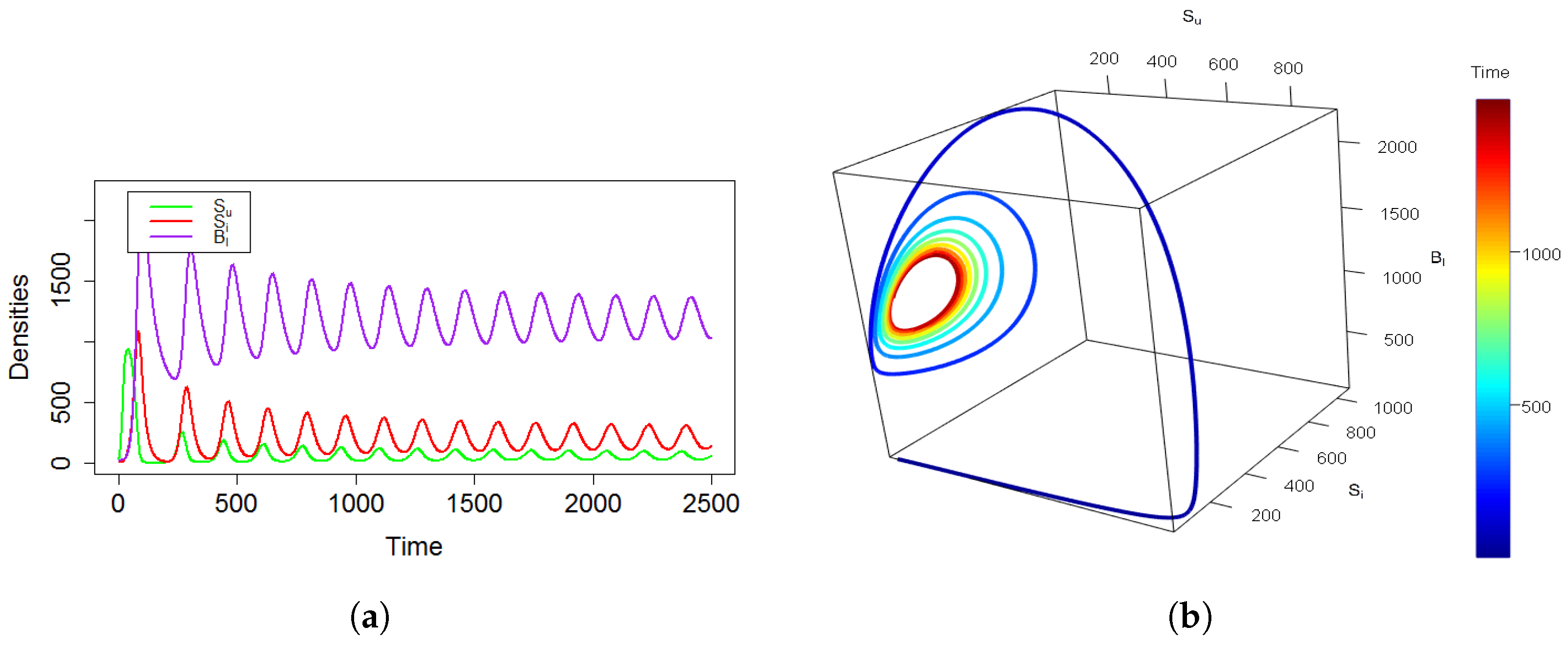
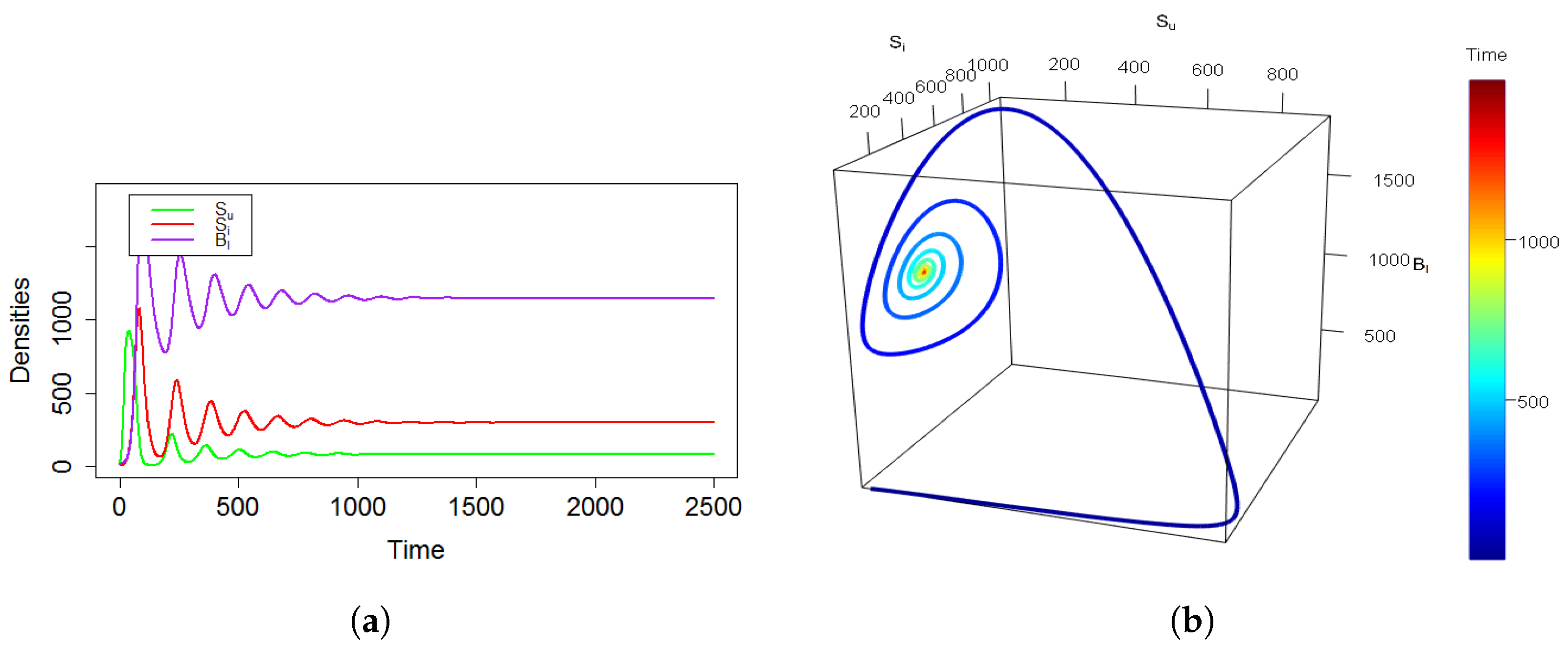
In Figure 1 and Figure 2, the behavior of the cell densities and the phase portrait diagrams of the healthy Schwann cells, infected Schwann cells and M. leprae bacteria for system (7) in the 3-D phase space are exhibited, respectively, for $\zeta =1$, i.e., for the classical integer-order system. Figure 1 depicts oscillatory periodic solutions and stable limit cycles. On the contrary, in Figure 2, stable solutions are observed whenever the value of ${\nu }_2$ is increased from $0.03$ to $0.05$, which describes that the intrinsic growth rate of the bacterial population is a very crucial parameter for demonstrating the dynamical shift in system (7).

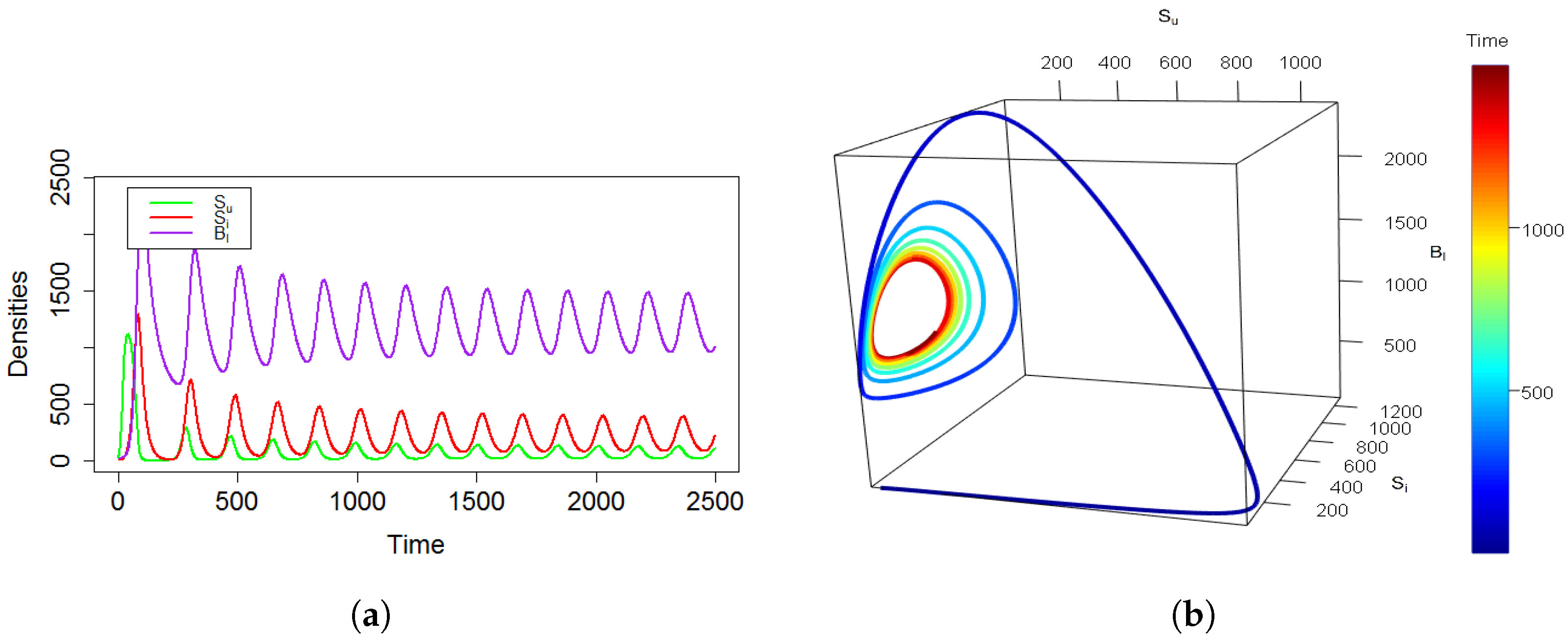
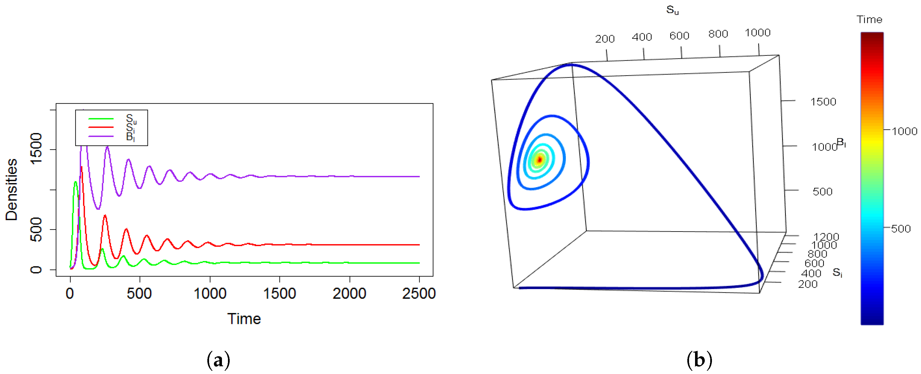
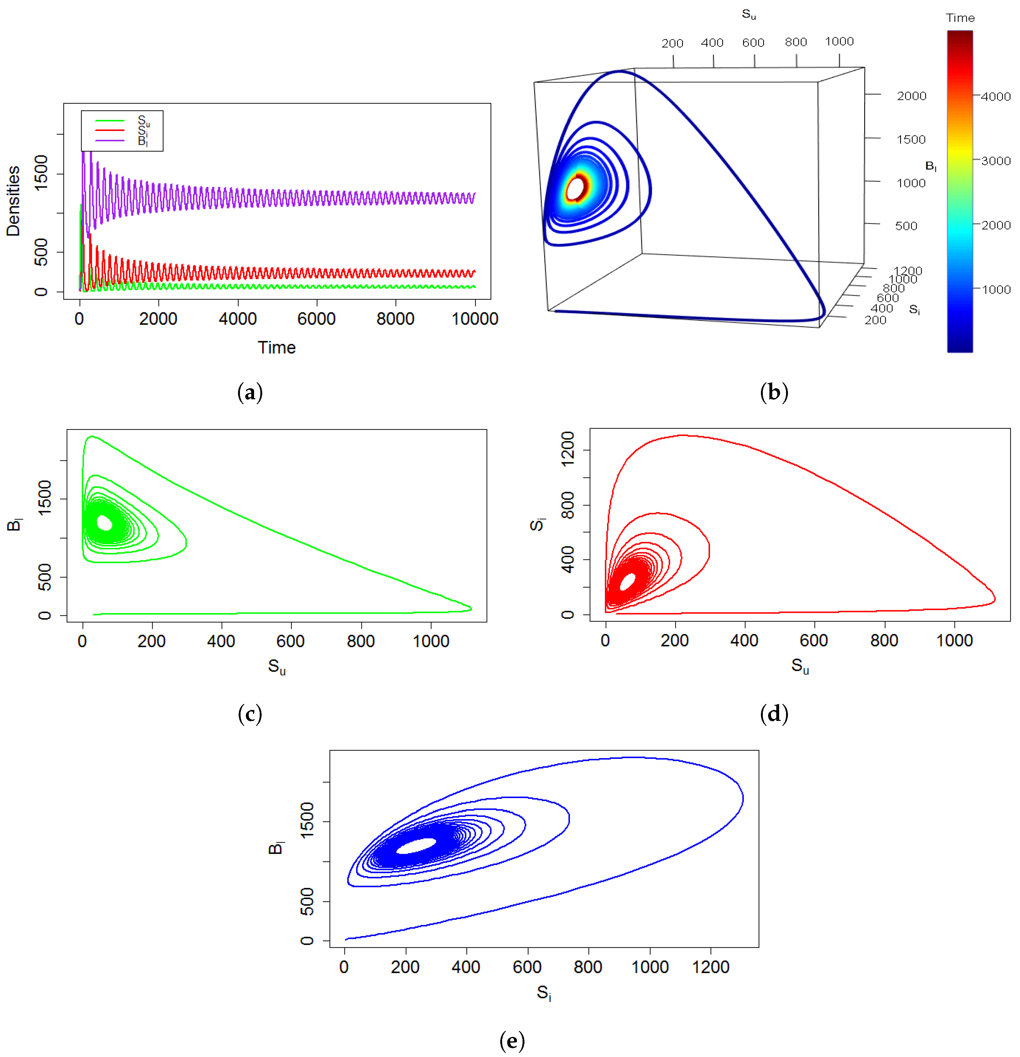
We now move on to understand the behavior of system (7) in the previous memory states, i.e., for the noninteger cases or fractional-order cases for the value of $\zeta \in (0,1)$. Considering $\zeta =0.8$, Figure 3 shows that system (7) produces oscillatory solutions and stable limit cycles for ${\nu }_2=0.03$, while $S_u$ cell, $S_i$ cell and $B_l$ bacteria reach the stable concentrations of approximately 50 mm${}^3$, 120 mm${}^3$ and 1100 mm${}^3$, respectively, at the endemic steady state $E^{*}$ described in Figure 4.

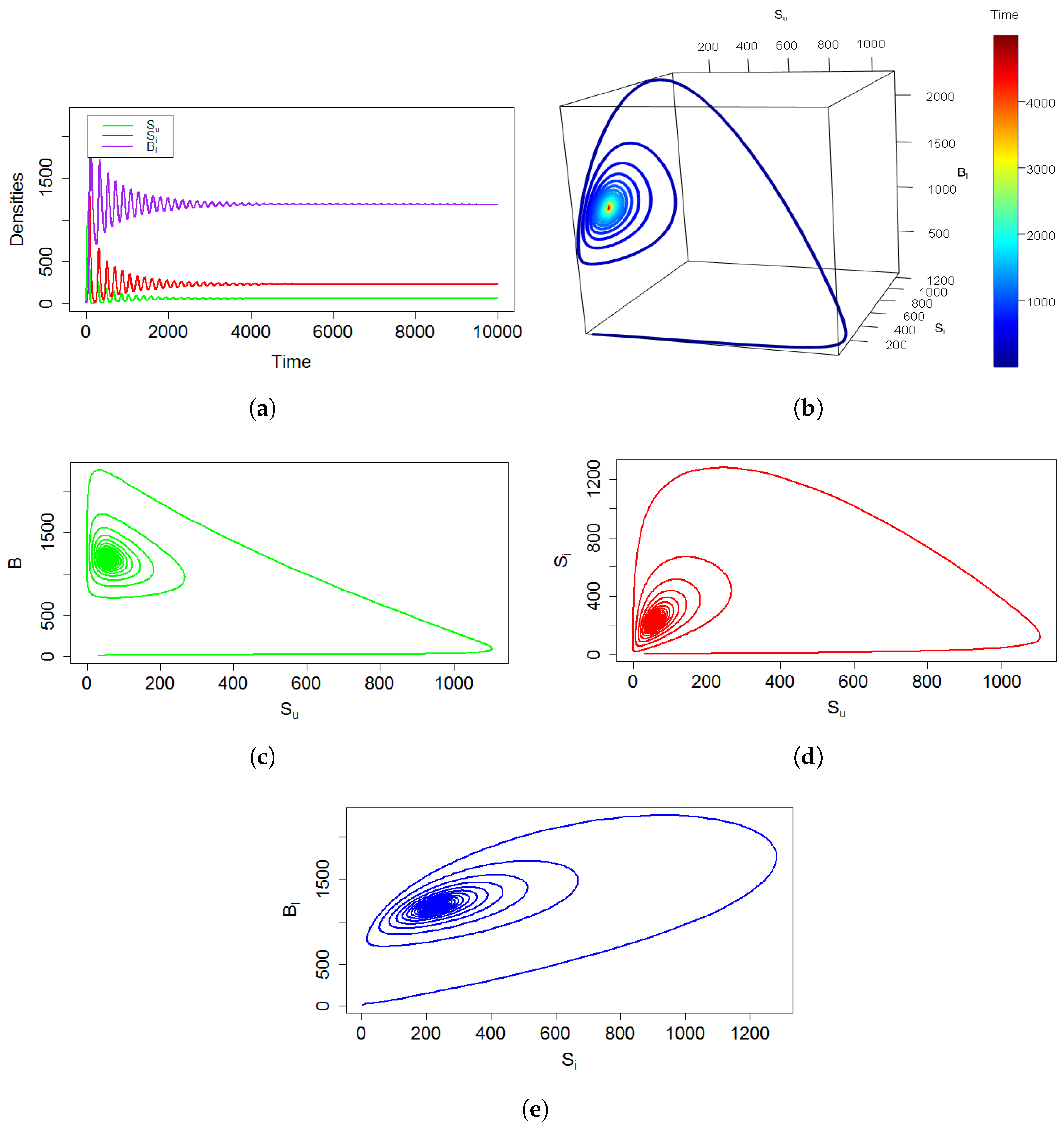
Next, a comparison of system (7)’s behavior is investigated for two different values of $\zeta$. Keeping the whole parameter set fixed, we varied the fractional order from $\zeta =1$ to $\zeta =0.6$. The numerical outcomes in Figure 5 exhibit unstable behavior with sustained oscillations of the cell population densities of system (7) for $\zeta =1$, but moving towards the previous memory state for $\zeta =0.6$, Figure 6 shows that after a little initial fluctuation, the system state populations become asymptotically stable. 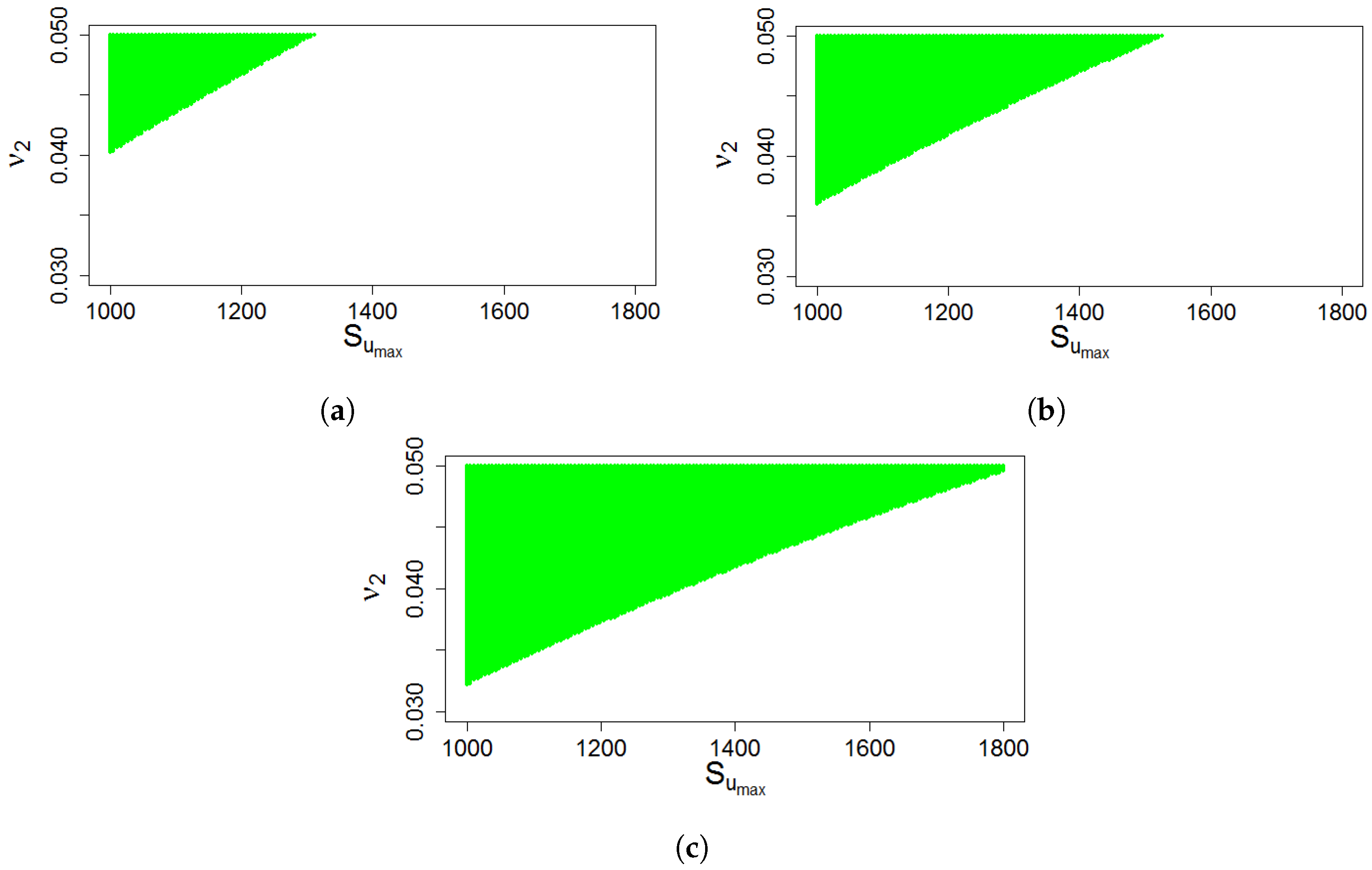In addition, in Figure 7, the stability regions of the interior equilibrium $E^{*}(S_u^{*},S_i^{*},B_l^{*})$ for the CF fractionalized system (7) for three different values of $\zeta$, i.e., for $\zeta =1,0.8,0.6$, are clearly demonstrated in Figure 7a, Figure 7b and Figure 7c, respectively.

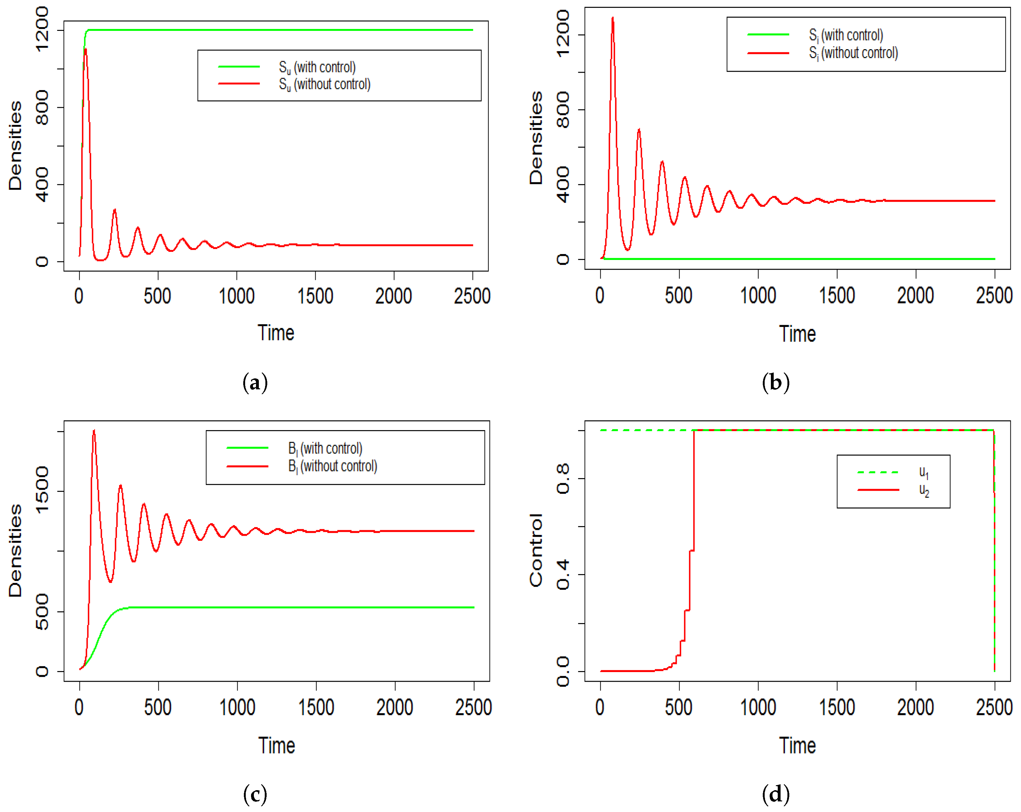
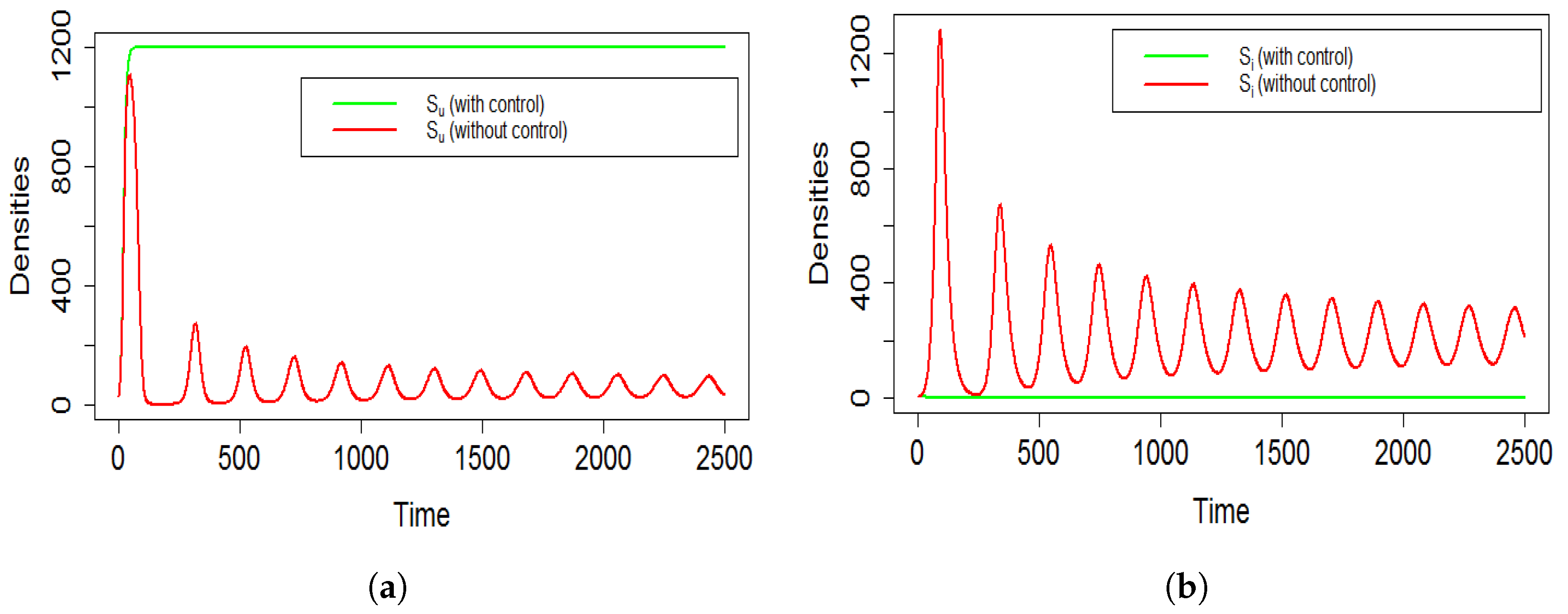
In Figure 8 and Figure 9, the effect of the optimal control treatment policy has been demonstrated on the Caputo–Fabrizio fractionalized optimal control (CFOC) system for the fractional orders $\zeta =0.9$ and $\zeta =0.6$, respectively. In both cases, the concentrations of healthy Schwann cells ($S_u$) are observed to be increased, and also the densities of $S_i$ and $B_l$ are decreased in the body of a leprosy-infected person. The bacterial concentration $B_l$ decreases to 510 mm${}^3$ in Figure 8c, while it decreases to a stable concentration of 420 mm${}^3$ depicted in Figure 9c. This indicates that the CFOC system (27) acts better when more previous memory states are considered for $\zeta =0.6$. 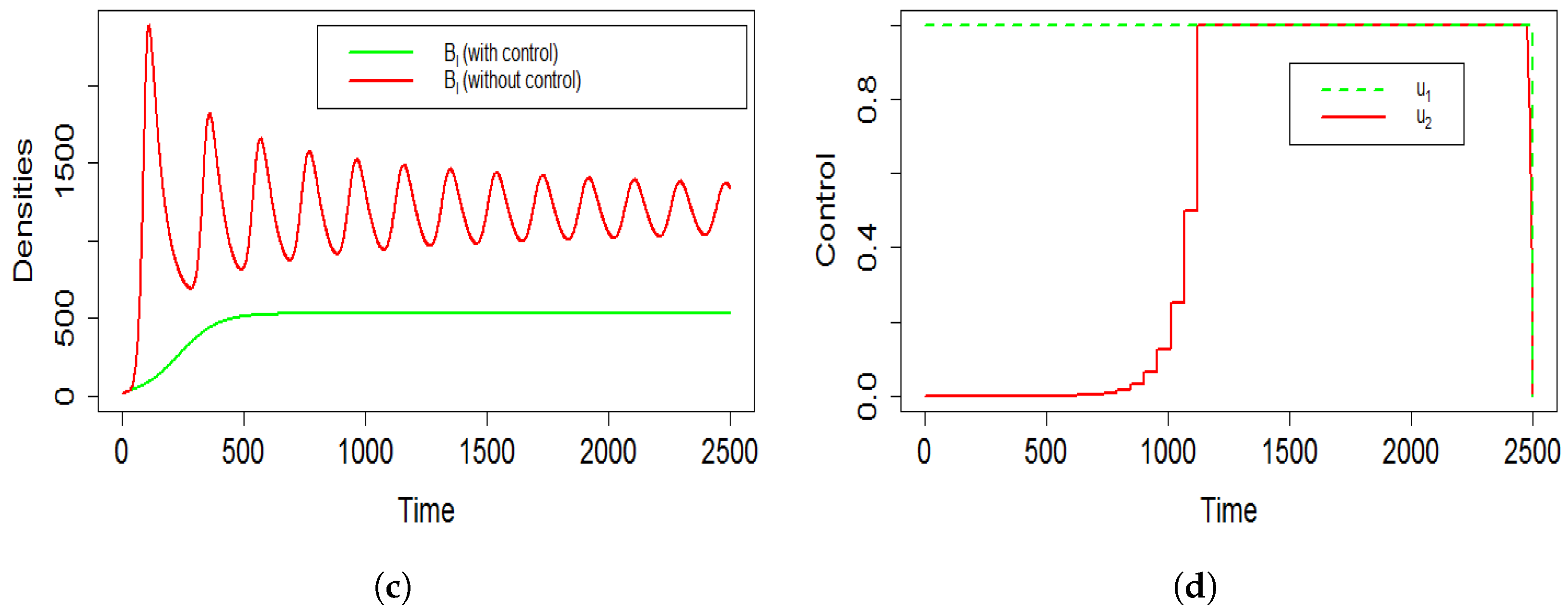Now, looking into the optimal control profiles of $u_1^{*}$ and $u_2^{*}$, we can see that the drug therapy Dapsone denoted by $u_2^{*}\left(t\right)$ needs to be increased after 520 days in case of $\zeta =0.9$, while it should be increased after nearly 1100 days up to the range 0.8–0.9 for $\zeta =0.6$ described in Figure 8d and Figure 9d, respectively. This happens due to the memory effect of M. leprae-induced infection and as the previous memory stages of the bacteria are extremely correlated with the drug resistance scenarios during the treatment [7]. Indeed, the M. leprae bacteria are highly Dapsone-resistant [39,54]. To tackle the dissemination of leprosy into the human body and to effectively inhibit bacterial drug resistance, applying the optimal control treatment approach for the previous memory state of $\zeta =0.6$ is more realistic in nature and appropriate than the present state or the states very adjacent to $\zeta =0.9$.

7. Discussion and Conclusions

Leprosy is a chronic infectious bacterial disease caused by the bacterium M. leprae. Despite several attempts by clinical and experimental scientists in the past, complete elimination of leprosy has still not been attained. The drug resistance characteristics of the bacterium, its associated relapse problems, and designing a perfect drug dose regimen in a cost-effective way remain a great challenge [37,55,56] for researchers worldwide. Applications of new innovative tools and techniques are essential in this situation. Keeping this in mind, we have formulated and analyzed a three-dimensional CF fractional-order-based mathematical system and, most importantly, investigated the impacts of memory effects on the CF fractionalized optimal control system by incorporating a combined drug therapy of Ofloxacin and Dapsone. In this section, we will discuss the crucial interpretations obtained from the analytical and numerical outcomes for both system (7) and system (27).

Firstly, we formulated an iterative scheme using the Laplace and inverse Laplace transformations in Section 3.1. Following that, we established the stability of the solutions using Picard’s T-stability iterative criterion in Theorem 2 in Section 3.2. For demonstrating the existence and uniqueness of the solutions (Theorem 3 in Section 3.3 and Section 3.4) of system (7), we used the well-known Banach fixed-point theorem and Arzela–Ascoli theorem. The formula for the basic reproduction number $R_0$ was derived and the local asymptotic stability of $E_0$ for the CF fractionalized system (7) was investigated with respect to the threshold value of $R_0=1$. Besides this, we also described the stability criterion of the endemic equilibrium $E^{*}$ of system (7) in Theorem 5 in Section 4. Furthermore, the CFOC system (27) was investigated by suitably defining the control set $\mathcal{U}$ in Equation (28) and the objective function (29) in Section 5. A generalized FOCP was formed in (31) and optimality conditions were proven in detail for this FOCP denoted by (42). Then, the formulas in (42) were applied to achieve the necessary and sufficient optimality conditions for system (27), and also the values of the optimal control pair $u_1^{*}$ and $u_2^{*}$ and the co-state or the adjoint equations with the corresponding transversality conditions were described elaborately in Theorem 7.

In 2021, Ghosh et al. [19] described three strategies and, among them, Strategy-III was found to be the most effective one. However, serious matters of concern in determining a realistic and accurate therapy for leprosy are the high cost and extreme adverse effects of the combined drug therapy. Here, in this research article, from Figure 8d and Figure 9d, we can observe that after introducing the memory effect, the amount of the drugs needed initially is much less for system (27) than for Strategy-III in both the memory-free model and integer-ordered system, which is much better in terms of cost-effectiveness and safe therapeutics.

Furthermore, comparing Figure 8 and Figure 9, we can notice that if the value of $\zeta$ is decreased from $0.9$ to $0.6$, oscillatory solutions appear for the specific range of the parameter set, but in both cases, under the optimal treatment policy, the densities of the cell populations approach a stable concentration. The dynamics of the optimal control profile of Ofloxacin remain almost similar for both $\zeta =0.9,0.6$, but the control profile of Dapsone provides notable differences. More specifically, for $\zeta =0.6$, the drug dose of Dapsone, i.e., $u_2^{*}\left(t\right)$, needs to be increased after 1100 days to tackle the highly Dapsone-drug-resistant M. leprae [39,54] and the associated infection procedure. Thus, to build a perfect regimen for combined therapy, acquiring enough knowledge from the previous memory states about drug-resistance issues [38,57,58] is essential and, hence, CFOC system (27) with $\zeta =0.6$ is very fruitful in this context. The more we reduce the value of $\zeta$ and approach the previous memory states, the more accurate the precision will be. Still, future works on leprosy in this aspect should also focus on investigating the memory stages for the value of $\zeta <0.6$, and before implementation, the outcomes should be validated properly by clinical and experimental researchers.

The memory effect for a biological problem actually involves the entire history before the present instant, and the implication of fractional calculus can be viewed as a suitable and exclusive tool for modeling these types of phenomena with hysteresis. Our present study reveals that the whole M. leprae-induced infection in leprosy not only depends on the present state but also on the previous memory stages of the infection process. With the different circumstances and effects that the whole infection mechanism experiences in various memory stages, the CF fractionalized system responds differently to the current conditions. The knowledge accumulated by the metabolic activities in preceding stages confers fitness to the bacteria in an evolutionary way, which validates that the history-dependent drug-resistant behavior is essentially a clear manifestation of the memory effect in leprosy. Thus, to overcome the drug resistance scenario, high-cost-related problems and side-effects of the combined therapy more accurately and realistically, the three-dimensional Caputo–Fabrizio fractionalized optimal control mathematical model (27) for the fractional order $\zeta =0.6$ presented in our research article should certainly be considered by mathematical and clinical scientists for all future studies on leprosy.

References

1. Schreuder, P.A.; Noto, S.; Richardus, J.H. Epidemiologic trends of leprosy for the 21st century. Clin. Dermatol. 2016, 34, 24–31. [Google Scholar] [CrossRef] [PubMed]
2. World Health Organization. Global leprosy situation, 2010. Wkly. Epidemiol. Rec. 2010, 85, 337–348. [Google Scholar]
3. World Health Organization. Global leprosy situation, 2012. Wkly. Epidemiol. Rec. 2012, 87, 317–328. [Google Scholar]
4. Ghosh, S.; Saha, S.; Roy, P.K. Critical observation of WHO recommended multidrug therapy on the disease leprosy through mathematical study. J. Theor. Biol. 2023, 567, 111496. [Google Scholar] [CrossRef] [PubMed]
5. Richardus, J.H.; Habbema, J.D.F. The impact of leprosy control on the transmission of M. leprae: Is elimination being attained? Lepr. Rev. 2007, 78, 330–337. [Google Scholar] [CrossRef] [PubMed]
6. Westerlund, S. Dead matter has memory! Phys. Scr. 1991, 43, 174. [Google Scholar] [CrossRef]
7. Wolf, D.M.; Fontaine-Bodin, L.; Bischofs, I.; Price, G.; Keasling, J.; Arkin, A.P. Memory in microbes: Quantifying history-dependent behavior in a bacterium. PLoS ONE 2008, 3, e1700. [Google Scholar] [CrossRef]
8. Yang, C.Y.; Bialecka-Fornal, M.; Weatherwax, C.; Larkin, J.W.; Prindle, A.; Liu, J.; Garcia-Ojalvo, J.; Süel, G.M. Encoding membrane-potential-based memory within a microbial community. Cell Syst. 2020, 10, 417–423. [Google Scholar] [CrossRef]
9. Samko, S.G.; Kilbas, A.A.; Marichev, O.I. Fractional Integrals and Derivatives; Gordon and Breach Science Publishers: Yverdon-les-Bains, Switzerland, 1993; Volume 1. [Google Scholar]
10. Miller, K.S.; Ross, B. An Introduction to the Fractional Calculus and Fractional Differential Equations; John Wiley & Sons: New York, NY, USA, 1993. [Google Scholar]
11. Ghosh, M.K.; Sardar, T.; Cao, X.; Roy, P.K. Mathematical study of a memory induced biochemical system. IEEE/CAA J. Autom. Sin. 2018, 5, 1142–1149. [Google Scholar] [CrossRef]
12. Rossikhin, Y.A.; Shitikova, M.V. Application of fractional calculus for dynamic problems of solid mechanics: Novel trends and recent results. Appl. Mech. Rev. 2010, 63, 010801. [Google Scholar] [CrossRef]
13. Stiassnie, M. On the application of fractional calculus for the formulation of viscoelastic models. Appl. Math. Model. 1979, 3, 300–302. [Google Scholar] [CrossRef]
14. Lundstrom, B.N.; Higgs, M.H.; Spain, W.J.; Fairhall, A.L. Fractional differentiation by neocortical pyramidal neurons. Nat. Neurosci. 2008, 11, 1335–1342. [Google Scholar] [CrossRef] [PubMed]
15. Caputo, M. Linear models of dissipation whose Q is almost frequency independent—II. Geophys. J. Int. 1967, 13, 529–539. [Google Scholar] [CrossRef]
16. Bagley, R.L.; Torvik, P.J. Fractional calculus-a different approach to the analysis of viscoelastically damped structures. AIAA J. 1983, 21, 741–748. [Google Scholar] [CrossRef]
17. Mathai, A.M.; Haubold, H.J. Special Functions for Applied Scientists; Springer: New York, NY, USA, 2008; Volume 4. [Google Scholar]
18. Kneller, G.R.; Hinsen, K. Fractional Brownian dynamics in proteins. J. Chem. Phys. 2004, 121, 10278–10283. [Google Scholar] [CrossRef] [PubMed]
19. Ghosh, S.; Chatterjee, A.N.; Roy, P.K.; Grigorenko, N.; Khailov, E.; Grigorieva, E. Mathematical Modeling and Control of the Cell Dynamics in Leprosy. Comput. Math. Model. 2021, 32, 52–74. [Google Scholar] [CrossRef]
20. Du, M.; Wang, Z.; Hu, H. Measuring memory with the order of fractional derivative. Sci. Rep. 2013, 3, 3431. [Google Scholar] [CrossRef]
21. Chinnathambi, R.; Rihan, F.A.; Alsakaji, H.J. A fractional-order model with time delay for tuberculosis with endogenous reactivation and exogenous reinfections. Math. Methods Appl. Sci. 2021, 44, 8011–8025. [Google Scholar] [CrossRef]
22. Al-Mdallal, Q.M.; Omer, A.S.A. Fractional-order Legendre-collocation method for solving fractional initial value problems. Appl. Math. Comput. 2018, 321, 74–84. [Google Scholar] [CrossRef]
23. Al-Mdallal, Q.M.; Hajji, M.A. A convergent algorithm for solving higher-order nonlinear fractional boundary value problems. Fract. Calc. Appl. Anal. 2015, 18, 1423–1440. [Google Scholar] [CrossRef]
24. Singh, J.; Kumar, D.; Baleanu, D. New aspects of fractional Biswas–Milovic model with Mittag–Leffler law. Math. Model. Nat. Phenom. 2019, 14, 303. [Google Scholar] [CrossRef]
25. Owolabi, K.M.; Atangana, A. Analysis and application of new fractional Adams–Bashforth scheme with Caputo–Fabrizio derivative. Chaos Solitons Fractals 2017, 105, 111–119. [Google Scholar] [CrossRef]
26. Kumar, D.; Singh, J.; Al Qurashi, M.; Baleanu, D. Analysis of logistic equation pertaining to a new fractional derivative with non-singular kernel. Adv. Mech. Eng. 2017, 9, 1–8. [Google Scholar] [CrossRef]
27. Tateishi, A.A.; Ribeiro, H.V.; Lenzi, E.K. The role of fractional time-derivative operators on anomalous diffusion. Front. Phys. 2017, 5, 52. [Google Scholar] [CrossRef]
28. Atangana, A.; Alkahtani, B.S.T. Analysis of the Keller–Segel model with a fractional derivative without singular kernel. Entropy 2015, 17, 4439–4453. [Google Scholar] [CrossRef]
29. Yang, L.; Su, Y.; Yang, X.; Wang, Z. The Optimal Control Strategy of Virus Transmission Based on Caputo-Fabrizio Order. Front. Phys. 2021, 9, 731972. [Google Scholar] [CrossRef]
30. Owolabi, K.M.; Patidar, K.C.; Shikongo, A. Numerical solution for a problem arising in angiogenic signalling. AIMS Math. 2019, 4, 43–63. [Google Scholar] [CrossRef]
31. Pontryagin, L.S. Mathematical Theory of Optimal Processes; CRC Press: Boca Raton, FL, USA, 1987. [Google Scholar]
32. Okyere, E.; Oduro, F.T.; Amponsah, S.K.; Dontwi, I.K. Fractional order optimal control model for malaria infection. arXiv 2016, arXiv:1607.01612. [Google Scholar]
33. Agrawal, O.P. A general formulation and solution scheme for fractional optimal control problems. Nonlinear Dyn. 2004, 38, 323–337. [Google Scholar] [CrossRef]
34. Agrawal, O.P. A formulation and numerical scheme for fractional optimal control problems. J. Vib. Control 2008, 14, 1291–1299. [Google Scholar] [CrossRef]
35. Agrawal, O.P.; Baleanu, D. A Hamiltonian formulation and a direct numerical scheme for fractional optimal control problems. J. Vib. Control 2007, 13, 1269–1281. [Google Scholar] [CrossRef]
36. Baba, B.A.; Bilgehan, B. Optimal control of a fractional order model for the COVID-19 pandemic. Chaos Solitons Fractals 2021, 144, 110678. [Google Scholar] [CrossRef] [PubMed]
37. Cambau, E.; Saunderson, P.; Matsuoka, M.; Cole, S.T.; Kai, M.; Suffys, P.; Rosa, P.S.; Williams, D.; Gupta, U.D.; Lavania, M.; et al. Antimicrobial resistance in leprosy: Results of the first prospective open survey conducted by a WHO surveillance network for the period 2009–15. Clin. Microbiol. Infect. 2018, 24, 1305–1310. [Google Scholar] [CrossRef] [PubMed]
38. Benjak, A.; Avanzi, C.; Singh, P.; Loiseau, C.; Girma, S.; Busso, P.; Fontes, A.N.B.; Miyamoto, Y.; Namisato, M.; Bobosha, K.; et al. Phylogenomics and antimicrobial resistance of the leprosy bacillus Mycobacterium leprae. Nat. Commun. 2018, 9, 352. [Google Scholar] [CrossRef]
39. Williams, D.L.; Araujo, S.; Stryjewska, B.M.; Scollard, D. Dapsone resistance in leprosy patients originally from American Samoa, United States, 2010–2012. Emerg. Infect. Dis. 2018, 24, 1584–1585. [Google Scholar] [CrossRef] [PubMed]
40. Matsuoka, M.; Budiawan, T.; Aye, K.S.; Kyaw, K.; Tan, E.V.; Cruz, E.D.; Gelber, R.; Saunderson, P.; Balagon, V.; Pannikar, V. The frequency of drug resistance mutations in Mycobacterium leprae isolates in untreated and relapsed leprosy patients from Myanmar, Indonesia and the Philippines. Lepr. Rev. 2007, 78, 343–352. [Google Scholar] [CrossRef]
41. Aubry, A.; Rosa, P.S.; Chauffour, A.; Fletcher, M.L.; Cambau, E.; Avanzi, C. Drug resistance in leprosy: An update following 70 years of chemotherapy. Infect. Dis. Now 2022, 52, 243–251. [Google Scholar] [CrossRef]
42. Ahuja, M.; Pathak, V.K. Ofloxacin resistance in multibacillary new leprosy cases from Purulia, West Bengal: A threat to effective secondary line treatment for rifampicin-resistant leprosy cases. J. Glob. Antimicrob. Resist. 2022, 30, 282–285. [Google Scholar] [CrossRef]
43. Vellappi, M.; Kumar, P.; Govindaraj, V.; Albalawi, W. An optimal control problem for mosaic disease via Caputo fractional derivative. Alex. Eng. J. 2022, 61, 8027–8037. [Google Scholar] [CrossRef]
44. Caputo, M.; Fabrizio, M. A new definition of fractional derivative without singular kernel. Prog. Fract. Differ. Appl. 2015, 1, 73–85. [Google Scholar]
45. Losada, J.; Nieto, J.J. Properties of a new fractional derivative without singular kernel. Prog. Fract. Differ. Appl. 2015, 1, 87–92. [Google Scholar]
46. Qing, Y.; Rhoades, B.E. T-stability of Picard iteration in metric spaces. Fixed Point Theory Appl. 2008, 2008, 418971. [Google Scholar] [CrossRef]
47. Gao, F.; Li, X.; Li, W.; Zhou, X. Stability analysis of a fractional-order novel hepatitis B virus model with immune delay based on Caputo-Fabrizio derivative. Chaos Solitons Fractals 2021, 142, 110436. [Google Scholar] [CrossRef]
48. Li, H.; Cheng, J.; Li, H.B.; Zhong, S.M. Stability analysis of a fractional-order linear system described by the Caputo–Fabrizio derivative. Mathematics 2019, 7, 200. [Google Scholar] [CrossRef]
49. Kamocki, R. Pontryagin maximum principle for fractional ordinary optimal control problems. Math. Methods Appl. Sci. 2014, 37, 1668–1686. [Google Scholar] [CrossRef]
50. Chatterjee, A.N.; Al Basir, F.; Almuqrin, M.A.; Mondal, J.; Khan, I. SARS-CoV-2 infection with lytic and non-lytic immune responses: A fractional order optimal control theoretical study. Results Phys. 2021, 26, 104260. [Google Scholar] [CrossRef]
51. Ghosh, S.; Rana, S.; Roy, P.K. Leprosy: Considering the Effects on Density-Dependent Growth of Mycobacterium leprae. Differ. Equations Dyn. Syst. 2022, 1–15. [Google Scholar] [CrossRef]
52. Masaki, T.; Qu, J.; Cholewa-Waclaw, J.; Burr, K.; Raaum, R.; Rambukkana, A. Reprogramming adult Schwann cells to stem cell-like cells by leprosy bacilli promotes dissemination of infection. Cell 2013, 152, 51–67. [Google Scholar] [CrossRef]
53. Khan, M.A.; Atangana, A. Modeling the dynamics of novel coronavirus (2019-nCov) with fractional derivative. Alex. Eng. J. 2020, 59, 2379–2389. [Google Scholar] [CrossRef]
54. Wu, Z.; Wang, C.; Wang, Z.; Shi, Y.; Jiang, H.; Wang, H. Risk factors for Dapsone Resistance in Leprosy Patients: A systematic meta-analysis. J. Glob. Antimicrob. Resist. 2022, 30, 459–467. [Google Scholar] [CrossRef]
55. Maymone, M.B.; Venkatesh, S.; Laughter, M.; Abdat, R.; Hugh, J.; Dacso, M.M.; Rao, P.N.; Stryjewska, B.M.; Dunnick, C.A.; Dellavalle, R.P. Leprosy: Treatment and management of complications. J. Am. Acad. Dermatol. 2020, 83, 17–30. [Google Scholar] [CrossRef] [PubMed]
56. Rosa, P.S.; D’Espindula, H.R.; Melo, A.C.; Fontes, A.N.; Finardi, A.J.; Belone, A.F.; Sartori, B.G.; Pires, C.A.; Soares, C.T.; Marques, F.B.; et al. Emergence and transmission of drug-/multidrug-resistant Mycobacterium leprae in a former leprosy colony in the brazilian amazon. Clin. Infect. Dis. 2020, 70, 2054–2061. [Google Scholar] [CrossRef] [PubMed]
57. Matsuoka, M. Drug resistance in leprosy. Jpn. J. Infect. Dis. 2010, 63, 1–7. [Google Scholar] [CrossRef] [PubMed]
58. Williams, D.L.; Gillis, T.P. Drug-resistant leprosy: Monitoring and current status. Lepr. Rev. 2012, 83, 269–281. [Google Scholar] [CrossRef]
Figure 1. Behavior of the solutions of the system populations and 3-D phase portrait diagrams of the CF fractionalized system (7) depicting the oscillatory dynamics and appearance of limit cycles for ζ = 1 . Values of ν 2 = 0.03 , S u m a x = 1000 were used to simulate the subfigures in this figure, where all the other parameter values were chosen from Table 1. (a) Behavior of the trajectories of system (7); (b) 3-D phase diagram for system (7) in S u S i B l space.
Mathematics 11 03630 g001
Figure 2. Behavior of the solutions of the system populations and 3-D phase portrait diagrams of the CF fractionalized system (7) depicting the stable behavior for ζ = 1 . Values of ν 2 = 0.05 and S u m a x = 1000 were used to simulate the subfigures in this figure where other parameter values were chosen from Table 1. (a) Behavior of the trajectories of system (7); (b) 3-D phase diagram for system (7) in S u S i B l space.
Mathematics 11 03630 g002
Figure 3. Time series and phase portrait diagram of the CF fractionalized system (7) depicting the unstable oscillatory behavior of the system state populations and appearance of stable limit cycles for ζ = 0.8 . Values of ν 2 = 0.03 and S u m a x = 1200 were used to simulate the subfigures in this figure where other parameter values were chosen from Table 1. (a) Behavior of the trajectories of system (7); (b) 3-D phase diagram for system (7) in S u S i B l space.
Mathematics 11 03630 g003
Figure 4. Time series and phase portrait diagram of the CF fractionalized system (7) depicting the asymptotically stable behavior of the system state populations for ζ = 0.8 . Here, values of ν 2 = 0.05 and S u m a x = 1200 were used to simulate the subfigures in this figure. Values of all the other parameters were chosen from Table 1. (a) Behavior of the trajectories of system (7); (b) 3-D phase diagram for system (7) in S u S i B l space.
Mathematics 11 03630 g004
Figure 5. Times series and phase portrait diagrams of the CF fractionalized system (7) depicting the sustained oscillatory unstable behavior of the system state populations and appearance of limit cycles for ζ = 1 . Here, values of ν 2 = 0.035 and S u m a x = 1200 were used for simulating the subfigures in this figure. All the other parameter values were chosen from Table 1. (a) Behavior of the trajectories of system (7); (b) 3-D phase diagram for system (7) in S u S i B l space; (c) 2-D phase diagram of system (7) in the S u B l plane; (d) 2-D phase diagram for system (7) in the S u S i plane; (e) 2-D phase diagram for system (7) in the S i B l plane.
Mathematics 11 03630 g005
Figure 6. Times series and phase portrait diagrams of the CF fractionalized system (7) depicting the asymptotically stable dynamics of the system state populations for ζ = 0.6 . Here, major observations are noted by studying the comparative behavior of system (7) between the CF-fractional order ζ = 1 (unstable in the form of stable periodic solutions and limit cycles shown in Figure 5) and ζ = 0.6 (stable behavior demonstrated in this figure, i.e., in Figure 6). Here, values of ν 2 = 0.035 and S u m a x = 1200 were used for simulating the subfigures in this figure. All the other parameter values were chosen from Table 1. (a) Behavior of the trajectories of system (7); (b) 3-D phase diagram for system (7) in S u S i B l space; (c) 2-D phase diagram of system (7) in the S u B l plane; (d) 2-D phase diagram for system (7) in the S u S i plane; (e) 2-D phase diagram for system (7) in the S i B l plane.
Mathematics 11 03630 g006
Figure 7. Representation of the stability regions for the Caputo–Fabrizio (CF) fractionalized system (7) for different values of CF fractional order ζ . Values of the parameters were chosen as ν 1 = 0.4 , B l m a x = 530 , μ = 0.1 , β 1 = 0.00032 , σ = 0.3 , β 2 = 0.00024 and all the values of other parameters were taken from Table 1. (a) Stability region for CF fractional order ζ = 1 ; (b) stability region for CF fractional order ζ = 0.8 ; (c) stability region for CF fractional order ζ = 0.6 .
Mathematics 11 03630 g007
Figure 8. Trajectories of the cell populations of the optimal-control-induced Caputo–Fabrizio fractional (CFOC) system (27). Scenarios for both with and without control are exhibited here in subfigures (a), (b) and (c), respectively, denoted by green and red color. In subfigure (d), optimal control profiles of u 1 * and u 2 * are shown for CFOC system (27). Values of the parameters were chosen as ζ = 0.9 , ν 2 = 0.03 , S u m a x = 1200 for simulating the subfigures of this figure and other parameter values were selected from Table 1. (a) Behavior of the densities of healthy Schwann cells S u ; (b) behavior of the densities of infected Schwann cells S i ; (c) behavior of the concentrations of M. leprae bacteria B l ; (d) dynamics of the optimal control profiles u 1 * and u 2 * for system (27).
Mathematics 11 03630 g008
Figure 9. Trajectories of the cell populations of the optimal-control-induced Caputo–Fabrizio fractional (CFOC) system (27). Scenarios for both with and without control are exhibited here in subfigures (a), (b) and (c), respectively, denoted by green and red colors. In subfigure (d), optimal control profiles of u 1 * and u 2 * are shown for CFOC system (27). Values of the parameters were chosen as ζ = 0.6 , ν 2 = 0.03 , S u m a x = 1200 for simulating the subfigures of this figure and other parameter values were selected from Table 1. (a) Behavior of the densities of healthy Schwann cells S u ; (b) behavior of the densities of infected Schwann cells S i ; (c) behavior of the concentrations of M. leprae bacteria B l ; (d) dynamics of the optimal control profiles u 1 * and u 2 * for system (27).
Mathematics 11 03630 g009aMathematics 11 03630 g009b