Birational Quadratic Planar Maps with Generalized Complex Rational Representations ^†

Abstract

Complex rational maps have been used to construct birational quadratic maps based on two special syzygies of degree one. Similar to complex rational curves, rational curves over generalized complex numbers have also been constructed by substituting the imaginary unit with a new independent quantity. We first establish the relationship between degree one, generalized, complex rational Bézier curves and quadratic rational Bézier curves. Then we provide conditions to determine when a quadratic rational planar map has a generalized complex rational representation. Thus, a rational quadratic planar map can be made birational by suitably choosing the middle Bézier control points and their corresponding weights. In contrast to the edges of complex rational maps of degree one, which are circular arcs, the edges of the planar maps can be generalized to hyperbolic and parabolic arcs by invoking the hyperbolic and parabolic numbers.

1. Introduction

A birational planar map is a rational function $\mathbf{p}(s,t)$ from ${\mathbb{R}}^2$ to ${\mathbb{R}}^2$ with a rational function ${\mathbf{p}}^{-1}(x,y)$ inverse to $\mathbf{p}(s,t)$, i.e., ${\mathbf{p}}^{-1}\left(\mathbf{p}(s,t)\right)=(s,t)$. The research on birational maps traces its history back to 1863 when birational maps were known as Cremona transformations. H. Hudson published a monograph in 1927 to classify Cremona transformations in the plane and in 3D space [1]. However, [1] predates by over half a century Bézier and B-spline curves and surfaces.

Free-form deformation (FFD) is an artist-friendly tool, which is used to model deformations by warping the ambient space [2]. FFD has numerous applications such as image morphing [3,4], facial animation [5] and medical image registration [6].

A preimage of a given $(x,y)$ is defined as any $(s,t)$ for which $\mathbf{p}(s,t)=(x,y)$. Computing FFD preimages is also required in many applications, e.g., extended FFD [7] and directly manipulated FFD [8]. However, computing preimages usually involves solving a system of nonlinear equations using either numerical methods or algebraic techniques. The computation of preimages can be simplified when the rational map used in FFD is birational. Hence, the notion of birational FFD is put forward in [9], i.e., an FFD in which the control points can be moved freely and the FFD can be made birational by adjusting the weights.

Birational FFDs of degree $1\times 1$, i.e., birational quadrilateral maps, are constructed by considering axial moving lines in [10]. The inverses of birational quadrilateral maps are also discussed from the viewpoint of generalized barycentric coordinates [11,12]. The relationship between the inverses of rational quadrilateral maps and their characteristic conic is presented in [13]. Hence, by setting the isoparametric curves to be monoid curves, Seberberg et al. [9] studied the construction of the birational 2D FFD of degree $1\times n$. To characterize the birational maps, Botbol et al. [14] provides a birationality criterion for bigraded birational maps. Note that the current methods to construct birational maps focus on the discussion of 2D rational maps related to bidegree cases [9,10].

Complex rational curves were introduced by J. Sánchez-Reyes by allowing complex weights in rational Bézier curves [15]. Based on the observation that complex rational curves have two special syzygies of low degrees [16], we can construct birational quadratic planar maps by exploiting their complex rational representations [17], which are complex rational maps of degree one. Complex rational planar maps of degree one represent exactly Möbius transformations. Based on Möbius transformations, Lipman et al. also introduced the four-point interpolant (FPI) maps, where four endpoints are free to move. Since Möbius transformations map lines to circles, the boundaries of the complex rational planar maps of degree one and FPI are limited circular arcs. Recently, the planar and bent corner-operated and transimilar (COTS) maps have been proposed to take the unit square to a region bounded by four log-spiral edges [18,19]. Based on the self-similar property of the log-spiral, the tiles of the COTS map of a regular pattern are similar, which will reduce the query cost of point inclusion testing (PIT) [20] and total area calculation (TAC). To increase the flexibility to construct birational planar maps and inspired by recent work on generalized complex rational curves [21], we shall discuss the construction of birational quadratic planar maps by probing their generalized complex representations. The main contributions of this study are as follows:

• We introduce generalized complex rational curves and planar maps, and we discuss their properties.
• We prove that degree one, generalized, complex rational maps correspond to quadratic birational planar maps.
• We propose a new method to construct quadratic birational planar maps via generalized complex rational planar maps.

This paper is organized in the following fashion. We begin in Section 2 by recalling some preliminary results about rational curves over generalized complex numbers. In Section 3, we establish the relationship between quadratic rational Bézier curves and degree one complex rational curves. By considering the bivariate case of generalized complex rational curves, we construct birational quadratic planar maps by degree one, generalized, complex rational maps in Section 4. We close in Section 5 with a brief summary of our work.

2. Rational Curves over Generalized Complex Numbers

2.1. Complex, Hyperbolic and Parabolic Numbers

Hyperbolic and parabolic numbers generalize complex numbers by introducing a new quantity $\alpha$: either ${\alpha }^2=-1$ (complex numbers), or ${\alpha }^2=+1$ (hyperbolic numbers), or ${\alpha }^2=0$ (parabolic numbers). The quantity $\alpha$ here is not a real number but an independent quantity. In addition, $\alpha$ commutes with every real number, and multiplication is associative and distributes through addition. Thus, we have the following multiplication rules:

$$\begin{array}{ccc}\hfill (a+b\alpha )(x+y\alpha )& =& (ax+by{\alpha }^2)+(ay+bx)\alpha \hfill \\ & =& \left\{\begin{array}{cc}(ax-by)+(ay+bx)\alpha ,\hfill & {\alpha }^2=-1;\hfill \\ (ax+by)+(ay+bx)\alpha ,\hfill & {\alpha }^2=1,\alpha \ne \pm 1;\hfill \\ \left(ax\right)+(ay+bx)\alpha ,\hfill & {\alpha }^2=0,\alpha \ne 0.\hfill \end{array}\right.\hfill \end{array}$$

The conjugate of $a+b\alpha$ is defined by

$$\begin{array}{c}\hfill \overline{a+b\alpha }=a-b\alpha .\end{array}$$

Multiplying a generalized complex number by its conjugate yields a real number, i.e., $\left(\overline{a+b\alpha }\right)(a+b\alpha )=a^2-b^2{\alpha }^2$. The modulus (or absolute value) of $a+b\alpha$ is defined by

$$\begin{array}{c}\hfill |a+b\alpha |=\sqrt{|\left(\overline{a+b\alpha }\right)(a+b\alpha )|}=\sqrt{|a^2-b^2{\alpha }^2|}.\end{array}$$

For generalized complex numbers, the analog of Euler’s formula is also true [22]. We have the following exponential formulas:

• (Complex numbers) $e^{\alpha t}=cos\left(t\right)+\alpha sin\left(t\right)$;
• (Hyperbolic numbers) $e^{\alpha t}=cosh\left(t\right)+\alpha sinh\left(t\right)$;
• (Parabolic numbers) $e^{\alpha t}=1+\alpha t$.

The exponential of generalized complex numbers represents either a rotation for complex numbers, a scissor shear for hyperbolic numbers [23] or a classical shear for parabolic numbers [24].

A generalized complex number can be identified with a point in the plane ${\mathbb{R}}^2$. Using the standard basis $\{1,\alpha \}$, we identify $a+b\alpha$ with the point or vector $(a,b)$. In analogy with complex numbers, we shall call the coefficient of 1 the real component and the coefficient of $\alpha$ the imaginary component of a hyperbolic or parabolic number.

The hyperbolic numbers can be used to help solve cubic Equations [25] and write Lorentz transformations in the special theory of relativity [22]. The parabolic numbers can be used to help analyze the mechanics of a mechanism [26].

2.2. Complex, Hyperbolic and Parabolic Rational Curves and Planar Maps

Generalized complex Bézier curves are defined by

$$\begin{array}{c}\hfill \mathbf{c}\left(s\right)=\frac{\mathbf{n}\left(s\right)}{\mathbf{d}\left(s\right)}=\frac{{\sum }_{i=0}^n{\mathbf{p}}_i{\mathbf{w}}_i{B}_i^n\left(s\right)}{{\sum }_{i=0}^n{\mathbf{w}}_i{B}_i^n\left(s\right)},s\in [0,1],\end{array}$$

(1)

where ${\mathbf{p}}_i=x_i+y_i\alpha$ are generalized complex control points, ${\mathbf{w}}_i=u_i+v_i\alpha$ are generalized complex weights and $B_i^n\left(s\right)=\frac{n!}{i!(n-i)!}{s}^i{(1-s)}^{n-i}$ are Bernstein polynomials. $\mathbf{c}\left(s\right)$ is called a complex, hyperbolic or parabolic rational Bézier curve when ${\alpha }^2=-1,+1,0$, respectively. By separating the real and imaginary parts of (1), we obtain

$$\begin{array}{c}\hfill \mathbf{c}\left(s\right)=\frac{n_0\left(s\right)+\alpha n_1\left(s\right)}{d_0\left(s\right)+\alpha d_1\left(s\right)},\end{array}$$

where $n_0\left(s\right),n_1\left(s\right),d_0\left(s\right),d_1\left(s\right)\in \mathbb{R}\left[s\right]$. Multiplying the numerator and denominator in (1) by the conjugate of the denominator yields

$$\begin{array}{c}\hfill \mathbf{c}\left(s\right)=\frac{\left(n_0{d}_0-{\alpha }^2{n}_1{d}_1\right)+\alpha \left(n_1{d}_0-n_0{d}_1\right)}{d_0^2-{\alpha }^2{d}_1^2}.\end{array}$$

(2)

Thus, c(s) corresponds to a real rational curve in the homogeneous form:

$$\begin{array}{c}\hfill \mathbf{C}\left(s\right)=\left(n_0{d}_0-{\alpha }^2{n}_1{d}_1,n_1{d}_0-n_0{d}_1,d_0^2-{\alpha }^2{d}_1^2\right).\end{array}$$

(3)

Note that when $n_0\left(s\right)n_1\left(s\right),d_0\left(s\right),d_1\left(s\right)$ are polynomials of degree n, i.e., c(s) is a generalized complex rational curve of degree n, its counterpart $\mathbf{C}\left(s\right)=\left(n_0{d}_0-{\alpha }^2{n}_1{d}_1,n_1{d}_0-n_0{d}_1,d_0^2-{\alpha }^2{d}_1^2\right)$ is a real rational curve of degree $2n$.

To discuss rational planar maps, we extend the generalized complex rational curves $\mathbf{c}\left(s\right)$ in 2D as follows:

$$\begin{array}{c}\hfill \mathbf{c}(s,t)=\frac{n_0(s,t)+\alpha n_1(s,t)}{d_0(s,t)+\alpha d_1(s,t)},\end{array}$$

(4)

where $n_0(s,t),n_1(s,t),d_0(s,t),d_1(s,t)\in \mathbb{R}[s,t]$. Recall that a syzygy of $\mathbf{Q}(t_1,t_2,\dots ,t_m)\in {\mathbb{R}}^k[t_1,t_2,\dots ,t_m]$ is a vector of polynomials

$$\mathbf{L}(t_1,t_2,\dots ,t_m)=\left(l_0(t_1,t_2,\dots ,t_m),l_1(t_1,t_2,\dots ,t_m),\dots ,l_{k-1}(t_1,t_2,\dots ,t_m)\right)$$

such that

$$\begin{array}{c}\hfill \mathbf{L}(t_1,t_2,\dots ,t_m)·\mathbf{Q}(t_1,t_2,\dots ,t_m)\equiv 0.\end{array}$$

Following the results in [21], we have the following observation

Lemma 1.

Given a rational planar map $\mathbf{C}(s,t)=(n_0{d}_0-{\alpha }^2{n}_1{d}_1,n_1{d}_0-n_0{d}_1,d_0^2-{\alpha }^2{d}_1^2)$ with generalized complex rational representation (4),

$$\begin{array}{c}\hfill \begin{array}{c}{\mathbf{L}}_0(s,t)=(d_0(s,t),{\alpha }^2{d}_1(s,t),-n_0(s,t)),\hfill \\ {\mathbf{L}}_1(s,t)=(d_1(s,t),d_0(s,t),-n_1(s,t)).\hfill \end{array}\end{array}$$

(5)

are two syzygies of $\mathbf{C}(s,t)$. Moreover, ${\mathbf{L}}_0(s,t)\times {\mathbf{L}}_1(s,t)=\mathbf{C}(s,t)$.

Proof. 

These results follow directly by substituting (5) into ${\mathbf{L}}_i(s,t)·\mathbf{C}(s,t),i=0,1$ and ${\mathbf{L}}_0(s,t)\times {\mathbf{L}}_1(s,t)$.    □

Note that the set of all syzygies of $\mathbf{C}(s,t)$ is also a free module of rank two over the ring $\mathbb{R}[s,t]$ (for more details, the interested reader is referred to the proof of Proposition 2.1 in [27]). Moreover, $\mu$-bases of generalized complex rational curves can be calculated via these syzygies in the one-dimensional case [16,21].

3. Generalized Complex Rational Linear Curves

Let ${\mathbf{p}}_l\left(s\right)$ denote the generalized complex rational Bézier curve of degree one:

$$\begin{array}{c}\hfill {\mathbf{p}}_l\left(s\right)=\frac{{\mathbf{w}}_0{\mathbf{p}}_0(1-s)+{\mathbf{w}}_1{\mathbf{p}}_{1}s}{{\mathbf{w}}_0(1-s)+{\mathbf{w}}_{1}s},s\in [0,1],\end{array}$$

(6)

where ${\mathbf{p}}_i=x_i+\alpha y_i$, ${\mathbf{w}}_i=u_i+\alpha v_i$, $i=0,1$. Note that when ${\mathbf{w}}_0,{\mathbf{w}}_1\in \mathbb{R}$, ${\mathbf{p}}_l\left(s\right)$ will degenerate to a line segment connecting ${\mathbf{p}}_0$ and ${\mathbf{p}}_1$. Hence, in the rest of this paper, we assume at least one of ${\mathbf{w}}_0,{\mathbf{w}}_1\notin \mathbb{R}$.

Lemma 2.

Let

$$\begin{array}{c}\hfill \mathbf{p}\left(s\right)=\frac{{\mathbf{p}}_0{w}_0{B}_0^2\left(s\right)+{\mathbf{p}}^{*}{w}^{*}{B}_1^2\left(s\right)+{\mathbf{p}}_1{w}_1{B}_2^2\left(s\right)}{w_0{B}_0^2\left(s\right)+w^{*}{B}_1^2\left(s\right)+w_1{B}_2^2\left(s\right)}\end{array}$$

(7)

be the corresponding real rational curve of ${\mathbf{p}}_l\left(s\right)$. Then, the control points and the weights in (7) have the following properties:

(1) 

$w_0={\mathbf{w}}_0{\overline{\mathbf{w}}}_0,w^{*}=({\mathbf{w}}_0{\overline{\mathbf{w}}}_1+{\mathbf{w}}_1{\overline{\mathbf{w}}}_0)/2,w_1={\mathbf{w}}_1{\overline{\mathbf{w}}}_1,w_0,w_1,w_2\in \mathbb{R};$

(2) 

${\mathbf{p}}^{*}=({\mathbf{w}}_0{\overline{\mathbf{w}}}_1{\mathbf{p}}_0+{\mathbf{w}}_1{\overline{\mathbf{w}}}_0{\mathbf{p}}_1)/({\mathbf{w}}_0{\overline{\mathbf{w}}}_1+{\overline{\mathbf{w}}}_0{\mathbf{w}}_1)=({\mathbf{w}}_0{\overline{\mathbf{w}}}_1{\mathbf{p}}_0+{\mathbf{w}}_1{\overline{\mathbf{w}}}_0{\mathbf{p}}_1)/\left(2w^{*}\right);$

(3) 

${\mathbf{p}}_1-{\mathbf{p}}^{*}=\frac{{\mathbf{w}}_0{\overline{\mathbf{w}}}_1}{2w^{*}}({\mathbf{p}}_1-{\mathbf{p}}_0)$, ${\mathbf{p}}^{*}-{\mathbf{p}}_0=\frac{{\overline{\mathbf{w}}}_0{\mathbf{w}}_1}{2w^{*}}({\mathbf{p}}_1-{\mathbf{p}}_0)$;

(4) 

$({\mathbf{p}}_1-{\mathbf{p}}^{*})/({\mathbf{p}}_1-{\mathbf{p}}_0)$ is the conjugate of $({\mathbf{p}}^{*}-{\mathbf{p}}_0)/({\mathbf{p}}_1-{\mathbf{p}}_0)$;

(5) 

${\mathbf{p}}^{*}=({\mathbf{p}}_0+{\mathbf{p}}_1)/2+\frac{{\overline{\mathbf{w}}}_0{\mathbf{w}}_1-{\mathbf{w}}_0{\overline{\mathbf{w}}}_1}{4w^{*}}({\mathbf{p}}_1-{\mathbf{p}}_0)=({\mathbf{p}}_0+{\mathbf{p}}_1)/2+{\lambda }^{*}({\mathbf{p}}_1-{\mathbf{p}}_0)\alpha$, where

$$\begin{array}{c}\hfill {\lambda }^{*}=\frac{u_1{v}_0-u_0{v}_1}{-2(u_0{u}_1+{\alpha }^2{v}_0{v}_1)};\end{array}$$

(8)

(6) 

Geometrically, ${\mathbf{p}}^{*}$ is on three different lines when ${\alpha }^2$ is set to $-1,+1,0$. All three lines pass through a common point $({\mathbf{p}}_0+{\mathbf{p}}_1)/2$. More precisely,

(a) 

When ${\alpha }^2=-1$, the line is the perpendicular bisector of the line segment between ${\mathbf{p}}_0$ and ${\mathbf{p}}_1$;

(b) 

When ${\alpha }^2=1$, the line is symmetric to the line ${\mathbf{p}}_0{\mathbf{p}}_1$ about the axis $({\mathbf{p}}_0+{\mathbf{p}}_1)/2+(1+\alpha )t,t\in \mathbb{R}$;

(c) 

When ${\alpha }^2=0$, the line is parallel to the y-axis, which also passes through the midpoint $({\mathbf{p}}_0+{\mathbf{p}}_1)/2$.

(7) 

The weight $w^{*}$ satisfies

$$\begin{array}{c}\hfill {\left(w^{*}\right)}^2=\frac{w_0{w}_1}{1-4{\alpha }^2{\left({\lambda }^{*}\right)}^2}.\end{array}$$

Proof. 

Items (1), (2), and (3) can be verified by multiplying the denominator and numerator of (6) by ${\overline{\mathbf{w}}}_0(1-s)+{\overline{\mathbf{w}}}_{1}s$.

Since the conjugate of $\frac{{\overline{\mathbf{w}}}_0{\mathbf{w}}_1}{2w^{*}}$ is $\frac{{\mathbf{w}}_0{\overline{\mathbf{w}}}_1}{2w^{*}}$, it follows from (3) that $({\mathbf{p}}_1-{\mathbf{p}}^{*})/({\mathbf{p}}_1-{\mathbf{p}}_0)$ is the conjugate of $({\mathbf{p}}^{*}-{\mathbf{p}}_0)/({\mathbf{p}}_1-{\mathbf{p}}_0)$. Hence, (4) holds.

Again, according to (3),

$$\begin{array}{c}\hfill ({\mathbf{p}}_1-{\mathbf{p}}^{*})-({\mathbf{p}}^{*}-{\mathbf{p}}_0)=({\mathbf{p}}_0+{\mathbf{p}}_1)-2{\mathbf{p}}^{*}=\frac{{\mathbf{w}}_0{\overline{\mathbf{w}}}_1-{\overline{\mathbf{w}}}_0{\mathbf{w}}_1}{2w^{*}}({\mathbf{p}}_1-{\mathbf{p}}_0).\end{array}$$

(9)

By solving for ${\mathbf{p}}^{*}$ in (9), we obtain ${\mathbf{p}}^{*}=({\mathbf{p}}_0+{\mathbf{p}}_1)/2+\frac{{\overline{\mathbf{w}}}_0{\mathbf{w}}_1-{\mathbf{w}}_0{\overline{\mathbf{w}}}_1}{4w^{*}}({\mathbf{p}}_1-{\mathbf{p}}_0)$. Substituting ${\mathbf{w}}_i=u_i+\alpha v_i$, $i=0,1$ into $\frac{{\overline{\mathbf{w}}}_0{\mathbf{w}}_1-{\mathbf{w}}_0{\overline{\mathbf{w}}}_1}{4w^{*}}$ yields

$$\begin{array}{c}\hfill \frac{{\overline{\mathbf{w}}}_0{\mathbf{w}}_1-{\mathbf{w}}_0{\overline{\mathbf{w}}}_1}{4w^{*}}=\frac{(u_1{v}_0-u_0{v}_1)}{-2(u_0{u}_1+{\alpha }^2{v}_0{v}_1)}\alpha .\end{array}$$

By setting ${\lambda }^{*}=(u_1{v}_0-u_0{v}_1)/(-2(u_0{u}_1+{\alpha }^2{v}_0{v}_1))$, it follows from (9) that ${\mathbf{p}}^{*}=({\mathbf{p}}_0+{\mathbf{p}}_1)/2+{\lambda }^{*}({\mathbf{p}}_1-{\mathbf{p}}_0)\alpha .$ Thus, (5) holds.

We shall prove (6) based on (5). Since

$$\begin{array}{ccc}\hfill \frac{{\overline{\mathbf{w}}}_0{\mathbf{w}}_1-{\mathbf{w}}_0{\overline{\mathbf{w}}}_1}{4w^{*}}({\mathbf{p}}_1-{\mathbf{p}}_0)& =& {\lambda }^{*}\alpha \left((x_1-x_0)+(y_1-y_0)\alpha \right)\hfill \\ & =& {\lambda }^{*}((y_1-y_0){\alpha }^2+(x_1-x_0)\alpha ),\hfill \end{array}$$

corresponds to the vector ${\lambda }^{*}\left((y_1-y_0){\alpha }^2,(x_1-x_0)\right)\in {\mathbb{R}}^2$, it follows that

(a)

When ${\alpha }^2=-1$, the vector ${\lambda }^{*}\left(-(y_1-y_0){\alpha }^2,x_1-x_0\right)={\lambda }^{*}\left(-(y_1-y_0),x_1-x_0\right)$, which is perpendicular to the vector $(x_1-x_0,y_1-y_0)$. Thus, ${\mathbf{p}}^{*}$ is on the perpendicular bisector of the line segment between ${\mathbf{p}}_0$ and ${\mathbf{p}}_1$;

(b)

When ${\alpha }^2=1$, the vector ${\lambda }^{*}\left((y_1-y_0){\alpha }^2,x_1-x_0\right)={\lambda }^{*}\left(y_1-y_0,x_1-x_0\right)$. Hence, ${\mathbf{p}}^{*}-({\mathbf{p}}_0+{\mathbf{p}}_1)/2={\lambda }^{*}\left(y_1-y_0,x_1-x_0\right)$. Since the vector $\left(y_1-y_0,x_1-x_0\right)$ is symmetric to the vector ${\mathbf{p}}_1-{\mathbf{p}}_0=(x_1-x_0,y_1-y_0)$ about the axis $y=x$, it follows that ${\mathbf{p}}^{*}$ is on a line symmetric to the line ${\mathbf{p}}_0{\mathbf{p}}_1$ about the axis $({\mathbf{p}}_0+{\mathbf{p}}_1)/2+t(1,1),t\in \mathbb{R}$;

(c)

When ${\alpha }^2=0$, the vector ${\lambda }^{*}\left((y_1-y_0){\alpha }^2,x_1-x_0\right)={\lambda }^{*}\left(0,x_1-x_0\right)$. Hence, ${\mathbf{p}}^{*}=(x_0+x_1,y_0+y_1)/2+{\lambda }^{*}\left(0,(x_1-x_0)\right)$, which is on a line parallel to the y-axis.

Next, we shall prove (7). Recall from (8) that ${\lambda }^{*}=\frac{u_1{v}_0-u_0{v}_1}{-2(u_0{u}_1+{\alpha }^2{v}_0{v}_1)}\in \mathbb{R}$. On the other hand,

$$\begin{array}{c}\hfill w^{*}=({\mathbf{w}}_0{\overline{\mathbf{w}}}_1+{\mathbf{w}}_1{\overline{\mathbf{w}}}_0)/2=u_0{u}_1-{\alpha }^2{v}_0{v}_1,w_0{w}_1=(u_0^2-{\alpha }^2{v}_0^2)(u_1^2-{\alpha }^2{v}_1^2).\end{array}$$

Hence, when $u_0{u}_1-{\alpha }^2{v}_0{v}_1\ne 0$,

$$\begin{array}{c}\hfill 1-4{\alpha }^2{\left({\lambda }^{*}\right)}^2=1-{\alpha }^2\frac{{(u_1{v}_0-u_0{v}_1)}^2}{{(u_0{u}_1-{\alpha }^2{v}_0{v}_1)}^2}=\frac{w_0{w}_1}{{\left(w^{*}\right)}^2}.\end{array}$$

Thus, ${\left(w^{*}\right)}^2=\frac{w_0{w}_1}{1-4{\alpha }^2{\left({\lambda }^{*}\right)}^2}$ and (7) holds.    □

Based on the above analysis, we are now ready to derive conditions for a general real rational quadratic Bézier curve to have a generalized complex rational representation.

Theorem 1.

Suppose that the two endpoints ${\mathbf{p}}_0,{\mathbf{p}}_1$ and their weights $w_0,w_1>0$ are fixed for the rational quadratic curve (7). If the middle control point and its weight satisfy the following two conditions:

(1) 

${\mathbf{p}}^{*}$ can be expressed as ${\mathbf{p}}^{*}=({\mathbf{p}}_0+{\mathbf{p}}_1)/2+\alpha ({\mathbf{p}}_1-{\mathbf{p}}_0)\lambda$ for some $\lambda \in \mathbb{R}$;

(2) 

$w^{*}$ can be expressed as

$$\begin{array}{c}\hfill w^{*}=\sqrt{\frac{w_0{w}_1}{1-4{\alpha }^2{\lambda }^2}},\end{array}$$

(10)

then $\mathbf{p}\left(s\right)$ has a generalized complex rational representation.

Proof. 

When the middle control point and its corresponding weight satisfy conditions (1) and (2), it can be verified that $\mathbf{p}\left(s\right)$ corresponds to a generalized complex rational representation $\frac{{\mathbf{w}}_0{\mathbf{p}}_0(1-s)+{\mathbf{w}}_0{\mathbf{z}}_0{\mathbf{p}}_{1}s}{{\mathbf{w}}_0(1-s)+{\mathbf{w}}_0{\mathbf{z}}_{0}s}$ if we choose ${\mathbf{w}}_0$ such that ${\mathbf{w}}_0{\overline{\mathbf{w}}}_0=w_0$ and set

$$\begin{array}{c}\hfill {\mathbf{w}}_1={\mathbf{w}}_0{\mathbf{z}}_0,\end{array}$$

(11)

where

$$\begin{array}{c}\hfill {\mathbf{z}}_0=\left\{\begin{array}{cc}\left(w^{*}+\alpha \sqrt{\left({\left(w^{*}\right)}^2-w_0{w}_1\right){\alpha }^2}\right)/w_0,\hfill & {\alpha }^2=\pm 1,\hfill \\ \left(w^{*}(1+2\lambda \alpha )\right)/w_0,\hfill & {\alpha }^2=0.\hfill \end{array}\right.\end{array}$$

(12)

   □

Remark 1.

Based on Theorem 1, a rational quadratic Bézier curve $\mathbf{p}\left(s\right)$ in (7) with complex rational representation is fully determined by ${\mathbf{p}}_0,{\mathbf{p}}_1$, $w_0,w_1$ and the parameter λ. To ensure that the curve segment is located in the convex hull of the control polygon ${\mathbf{p}}_0{\mathbf{p}}_1{\mathbf{p}}_2$, we shall adopt the positive square root for $w^{*}$ in (10). 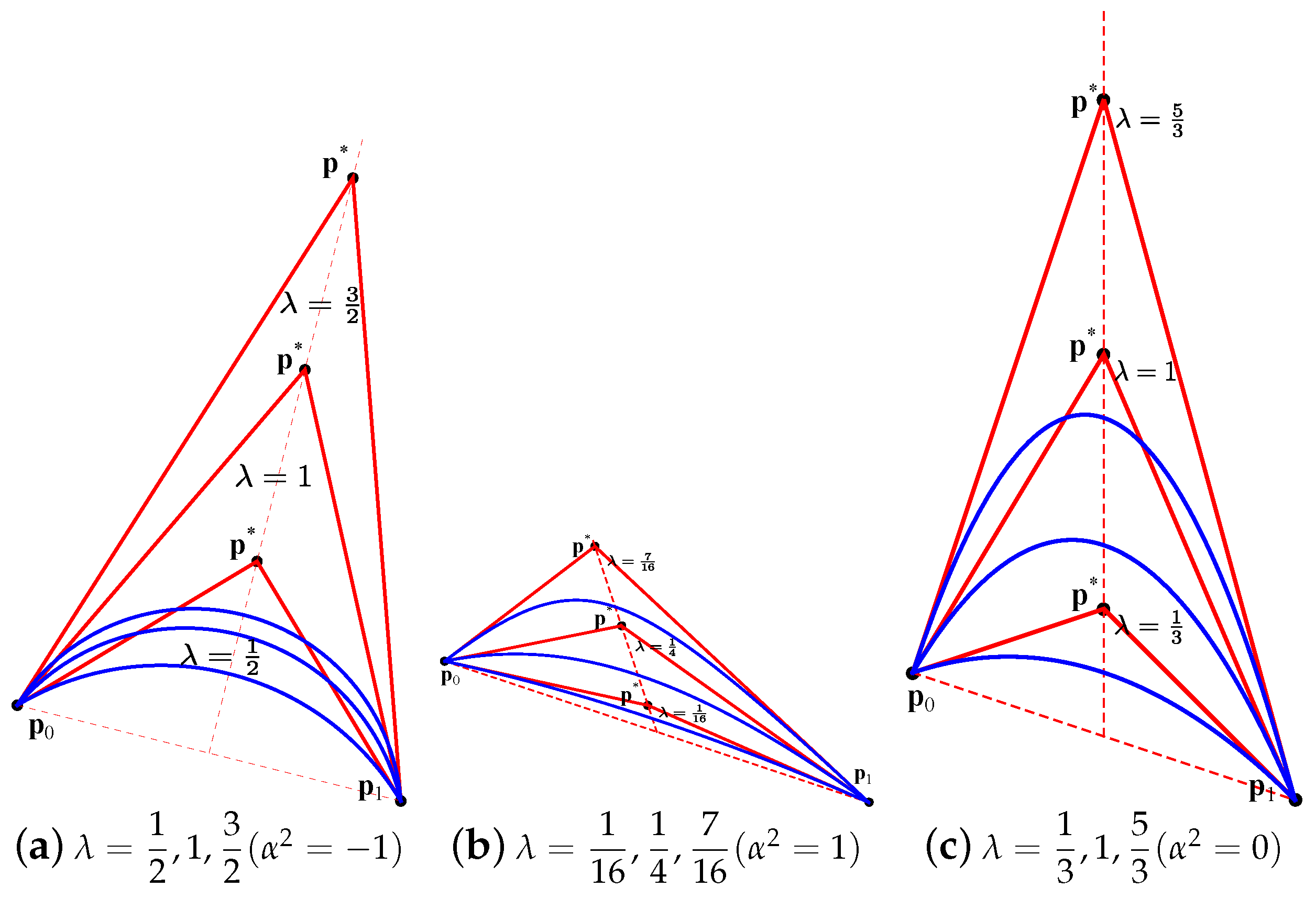The complementary segment of the curve is generated by reversing of the sign of $w^{*}$ [28].

Remark 2.

When $w_0\ne 0$, we can divide the numerator and the denominator of ${\mathbf{p}}_l\left(s\right)$ by ${\mathbf{w}}_0$. Hence, ${\mathbf{p}}_l\left(s\right)$ can be rewritten as

$$\begin{array}{c}\hfill {\mathbf{p}}_l\left(s\right)=\frac{{\mathbf{p}}_0(1-s)+{\mathbf{w}}_1/{\mathbf{w}}_0{\mathbf{p}}_{1}s}{(1-s)+{\mathbf{w}}_1/{\mathbf{w}}_{0}s}=\frac{{\mathbf{p}}_0(1-s)+{\mathbf{z}}_0{\mathbf{p}}_{1}s}{(1-s)+{\mathbf{z}}_{0}s}.\end{array}$$

Thus, the choice of the ratio ${\mathbf{z}}_0={\mathbf{w}}_1/{\mathbf{w}}_0$, instead of ${\mathbf{w}}_0$ itself, affects the shape of the curve $\mathbf{p}\left(s\right)$.

Remark 3.

$z_0$ in (12) can be expressed in exponential form:

$$\begin{array}{c}\hfill {\mathbf{z}}_0=\left\{\begin{array}{cc}\sqrt{{\displaystyle \frac{w_1}{w_0}}}{e}^{\alpha arctan\left(2\lambda \right)},\hfill & {\alpha }^2=-1;\hfill \\ \sqrt{{\displaystyle \frac{w_1}{w_0}}}{e}^{\alpha artanh\left(2\lambda \right)},\hfill & {\alpha }^2=1;\hfill \\ \sqrt{{\displaystyle \frac{w_1}{w_0}}}{e}^{\alpha \left(2\lambda \right)},\hfill & {\alpha }^2=0.\hfill \end{array}\right.\end{array}$$

Remark 4.

In the case of hyperbolic rational curves, since ${\alpha }^2=1$, it follows from (10) that the parameter λ must satisfy: $\lambda \in (-1/2,1/2)$.

Example 1.

(${\alpha }^2=-1$) Consider two endpoints ${\mathbf{p}}_0=(2,1),{\mathbf{p}}_1=(5,0)$ and their corresponding weights $w_0=4,w_1=9$. Choose ${\mathbf{p}}^{*}=({\mathbf{p}}_0+{\mathbf{p}}_1)/2+\alpha ({\mathbf{p}}_1-{\mathbf{p}}_0)\lambda$ with $\lambda =1/2,1,3/2$. From (10), we need to set the weight $w^{*}$:

$$\begin{array}{c}\hfill w^{*}=\sqrt{\frac{w_0{w}_1}{1-4{\lambda }^2{\alpha }^2}}=3\sqrt{2},\frac{6}{\sqrt{5}},3\sqrt{\frac{2}{5}}.\end{array}$$

Choose ${\mathbf{w}}_0=1+\alpha \sqrt{3}$. Then, ${\mathbf{w}}_1=-\frac{3\left(-1+\sqrt{3}\right)}{2\sqrt{2}}+\frac{3}{4}\left(\sqrt{2}+\sqrt{6}\right)\alpha$, $\frac{3}{2}\left(\frac{1}{\sqrt{5}}-2\sqrt{\frac{3}{5}}\right)+$$\frac{3\left(2+\sqrt{3}\right)}{2\sqrt{5}}\alpha$, $\frac{3\left(1-3\sqrt{3}\right)}{2\sqrt{10}}+\frac{3\left(3+\sqrt{3}\right)}{2\sqrt{10}}\alpha$. The corresponding rational quadratic curves $\mathbf{p}\left(s\right)$ are shown in Figure 1a (blue curves).

Figure 1. Generalized complex rational curves of degree one. The control polygon (red color) and the corresponding curve (blue color) vary as the parameter $\lambda$ changes.

Example 2.

(${\alpha }^2=1$) Consider two endpoints ${\mathbf{p}}_0=(1,2),{\mathbf{p}}_1=(5,3)$ and their corresponding weights $w_0=3,w_1=9$. Choose ${\mathbf{p}}^{*}=({\mathbf{p}}_0+{\mathbf{p}}_1)/2+\alpha ({\mathbf{p}}_1-{\mathbf{p}}_0)\lambda$ with $\lambda =3/16,5/16,7/16$. From (10), we need to set the weight $w^{*}$:

$$\begin{array}{c}\hfill w^{*}=\sqrt{\frac{w_0{w}_1}{1-4{\alpha }^2{\lambda }^2}}=8\sqrt{\frac{3}{7}},6,\frac{24}{\sqrt{5}}.\end{array}$$

Let ${\mathbf{w}}_0=(2,1)$. Then, ${\mathbf{w}}_1=\frac{17}{\sqrt{21}}+\frac{10}{\sqrt{21}}\alpha ,5+4\alpha ,\frac{23}{\sqrt{5}}+\frac{22}{\sqrt{5}}\alpha$. The corresponding rational quadratic curves $\mathbf{p}\left(s\right)$ are shown in Figure 1b (blue curves).

Example 3.

(${\alpha }^2=0$) Consider two endpoints ${\mathbf{p}}_0=(1,2),{\mathbf{p}}_1=(5,3)$ and their corresponding weights $w_0=4,w_1=9$. Choose ${\mathbf{p}}^{*}=({\mathbf{p}}_0+{\mathbf{p}}_1)/2+\alpha ({\mathbf{p}}_1-{\mathbf{p}}_0)\lambda$ with $\lambda =1/3,1,5/3$. From (10), we need to set the weight $w^{*}$:

$$\begin{array}{c}\hfill w^{*}=\sqrt{\frac{w_0{w}_1}{1-4{\alpha }^2{\lambda }^2}}=6.\end{array}$$

Let ${\mathbf{w}}_0=(2,1)$. Then, ${\mathbf{w}}_1=3+\frac{7}{2}\alpha ,3+\frac{15}{2}\alpha ,3+\frac{23}{2}\alpha$. The corresponding rational quadratic curves $\mathbf{p}\left(s\right)$ are shown in Figure 1c (blue curves).

4. Construction of Quadratic Birational Maps via Generalized Complex Representations

To generate planar rational maps, we generalize ${\mathbf{p}}_l\left(s\right)$ in (6) to the bivariate setting as follows.

Consider three non-collinear endpoints ${\mathbf{p}}_{100},{\mathbf{p}}_{010},{\mathbf{p}}_{001}$. Let

$$\begin{array}{ccc}\hfill & {\mathbf{p}}_l(s,t)& =\frac{{\mathbf{p}}_{100}{\mathbf{w}}_{100}u+{\mathbf{p}}_{010}{\mathbf{w}}_{010}s+{\mathbf{p}}_{001}{\mathbf{w}}_{001}t}{{\mathbf{w}}_{100}u+{\mathbf{w}}_{010}s+{\mathbf{w}}_{001}t},\hfill \\ & & 0\le u,s,t\le 1,u=1-s-t,\hfill \end{array}$$

(13)

where ${\mathbf{w}}_{100},{\mathbf{w}}_{010},{\mathbf{w}}_{001}$ are generalized complex weights, denoted by

$$\begin{array}{ccc}\hfill & {\mathbf{w}}_{100}=u_0+\alpha v_0,{\mathbf{w}}_{010}=u_1+\alpha v_1,{\mathbf{w}}_{001}=u_2+\alpha v_2,& \\ & {\mathbf{p}}_{100}{\mathbf{w}}_{100}={\widehat{x}}_0+\alpha {\widehat{y}}_0,{\mathbf{p}}_{010}{\mathbf{w}}_{010}={\widehat{x}}_1+\alpha {\widehat{y}}_1,{\mathbf{p}}_{001}{\mathbf{w}}_{001}={\widehat{x}}_2+\alpha {\widehat{y}}_2.\end{array}$$

To avoid the degenerate case, we also assume ${\mathbf{w}}_{100}$, ${\mathbf{w}}_{010}$, ${\mathbf{w}}_{001}\ne 0$. In addition, at least one of ${\mathbf{w}}_{100}$, ${\mathbf{w}}_{010}$, ${\mathbf{w}}_{001}$ is not fully real throughout the rest of the paper. Note that the complex, hyperbolic and parabolic rational curves are invariant with respect to Möbius transformations, i.e., applying a Möbius transformation to the control points and weights is equivalent to applying the Möbius transformation to every point on the curve (for more details, the readers are referred to Theorem 4.5 in [21]).

Multiplying the numerator and denominator in (13) by the conjugate of the denominator yields the corresponding quadratic real rational planar map:

$$\begin{array}{c}\hfill \mathbf{p}(s,t)=\frac{{\sum }_{i+j+k=2}{\mathbf{p}}_{ijk}{w}_{ijk}{B}_{ijk}^2(u,s,t)}{{\sum }_{i+j+k=2}{w}_{ijk}{B}_{ijk}^2(u,s,t)},\end{array}$$

(14)

where $B_{ijk}^n(u,s,t)$ are Bernstein polynomials defined by

$$B_{ijk}^n(u,s,t)=\frac{n!}{i!j!k!}{u}^i{s}^j{t}^k,i+j+k=n,$$

and $w_{ijk}=({\mathbf{w}}_{i_1{j}_1{k}_1}\overline{{\mathbf{w}}_{i_2{j}_2{k}_2}}+\overline{{\mathbf{w}}_{i_1{j}_1{k}_1}}{\mathbf{w}}_{i_2{j}_2{k}_2})/2$,

$${\mathbf{p}}_{ijk}=({\mathbf{w}}_{i_1{j}_1{k}_1}\overline{{\mathbf{w}}_{i_2{j}_2{k}_2}}{\mathbf{p}}_{i_1{j}_1{k}_1}+\overline{{\mathbf{w}}_{i_1{j}_1{k}_1}}{\mathbf{w}}_{i_2{j}_2{k}_2}{\mathbf{p}}_{i_2{j}_2{k}_2})/\left(2w_{ijk}\right),$$

$(i,j,k)=(i_1+i_2,j_1+j_2,k_1+k_2),i_1+j_1+k_1=i_2+j_2+k_2=1$.

Denote by $\mathbf{P}(s,t)=\left(a(s,t),b(s,t),c(s,t)\right)$, the homogeneous form of $\mathbf{p}(s,t)=(\frac{a(s,t)}{c(s,t)},$$\frac{b(s,t)}{c(s,t)})$. Next, we shall derive the syzygies of a planar rational map $\mathbf{P}(s,t)$ that is endowed with a generalized complex representation (13).

From Lemma 1, there are two special syzygies ${\mathbf{L}}_0(s,t),{\mathbf{L}}_1(s,t)$ in the form (5) of $\mathbf{P}(s,t)$, which are $\mathbb{R}[s,t]$-independent. Let $l_0(x,y;s,t)={\mathbf{L}}_0(s,t)·(x,y,1)$ and $l_1(x,y;s,t)={\mathbf{L}}_0(s,t)·(x,y,1)$. Then, after calculation, we obtain

$$\begin{array}{c}\hfill \left(\begin{array}{c}{l}_0(x,y;s,t)\\ l_1(x,y;s,t)\end{array}\right)={\mathbf{m}}_{s}s+{\mathbf{m}}_{t}t+{\mathbf{m}}_0,\end{array}$$

where

$$\begin{array}{ccc}\hfill & {\mathbf{m}}_s& =\left(\begin{array}{c}x(u_1-u_0)+{\alpha }^{2}y(v_1-v_0)+({\widehat{x}}_1-{\widehat{x}}_0)\\ x(v_1-v_0)+y(u_1-u_0)+({\widehat{y}}_1-{\widehat{y}}_0)\end{array}\right),\hfill \\ & {\mathbf{m}}_t& =\left(\begin{array}{c}x(u_2-u_0)+{\alpha }^{2}y(v_2-v_0)+({\widehat{x}}_2-{\widehat{x}}_0)\\ x(v_2-v_0)+y(v_2-v_0)+({\widehat{y}}_2-{\widehat{y}}_0)\end{array}\right),\hfill \\ & {\mathbf{m}}_0& =\left(\begin{array}{c}x{u}_0+{\alpha }^{2}y{v}_0-{\widehat{x}}_0\\ x{v}_0+y{u}_0-{\widehat{y}}_0\end{array}\right).\hfill \end{array}$$

With the above notation in hand, we are now ready to give the inversion formulas for a rational quadratic map with a generalized complex rational representation.

Theorem 2.

For a real planar rational quadratic map $\mathbf{p}(s,t)$ with a generalized complex rational representation (13), the inversion equation is

$$\begin{array}{c}\hfill \left\{\begin{array}{c}s=det\left({\mathbf{M}}_1\right)/det\left({\mathbf{M}}_{\mathbf{0}}\right),\hfill \\ t=det\left({\mathbf{M}}_2\right)/det\left({\mathbf{M}}_{\mathbf{0}}\right),\hfill \end{array}\right.\end{array}$$

where

$$\begin{array}{c}\hfill {\mathbf{M}}_0=({\mathbf{m}}_s,{\mathbf{m}}_t),{\mathbf{M}}_1=({\mathbf{m}}_0,{\mathbf{m}}_t),{\mathbf{M}}_2=({\mathbf{m}}_s,{\mathbf{m}}_0).\end{array}$$

Hence, the rational map (13) with generalized complex rational representation is birational.

Proof. 

The proof is similar to the proof of Theorem 4 in [17].    □

Given three endpoints ${\mathbf{p}}_{200}$, ${\mathbf{p}}_{020}$, ${\mathbf{p}}_{002}$ and their corresponding weights $w_{200}$, $w_{020}$, $w_{002}>0$, next we shall show how to obtain ${\mathbf{p}}_{110},{\mathbf{p}}_{101},{\mathbf{p}}_{011}$ and $w_{110}$, $w_{101}$, $w_{011}$ such that the rational quadratic map is endowed with a generalized complex rational representation.

Note that not all three middle points are free to be chosen arbitrarily. Without loss of generality, we consider the two boundary curves $\mathbf{p}(s,0)$, $\mathbf{p}(0,t)$ first. Choose two parameters ${\lambda }_{110},{\lambda }_{101}\in \mathbb{R}$ to fix the middle points ${\mathbf{p}}_{110},{\mathbf{p}}_{101}$, i.e.,

$$\begin{array}{ccc}& {\mathbf{p}}_{110}=({\mathbf{p}}_{200}+{\mathbf{p}}_{020})/2+\alpha ({\mathbf{p}}_{200}-{\mathbf{p}}_{020}){\lambda }_{110},& \\ & {\mathbf{p}}_{101}=({\mathbf{p}}_{200}+{\mathbf{p}}_{002})/2+\alpha ({\mathbf{p}}_{200}-{\mathbf{p}}_{002}){\lambda }_{101}.\end{array}$$

Then from (10) in Theorem 1, we obtain

$$\begin{array}{c}\hfill w_{110}=\sqrt{\frac{w_{200}{w}_{020}}{1-4{\alpha }^2{\lambda }_{110}^2}},w_{101}=\sqrt{\frac{w_{200}{w}_{002}}{1-4{\alpha }^2{\lambda }_{101}^2}}.\end{array}$$

By setting the generalized complex weight ${\mathbf{w}}_{100}$ such that $w_{200}=\overline{{\mathbf{w}}_{100}}{\mathbf{w}}_{100}$, we can compute ${\mathbf{w}}_{010}$, ${\mathbf{w}}_{001}$ from (11).

Let ${\mathbf{p}}_{100}={\mathbf{p}}_{200},{\mathbf{p}}_{010}={\mathbf{p}}_{020},{\mathbf{p}}_{001}={\mathbf{p}}_{002}$, then

$$\begin{array}{ccc}& w_{011}=& ({\mathbf{w}}_{010}\overline{{\mathbf{w}}_{001}}+{\mathbf{w}}_{010}\overline{{\mathbf{w}}_{001}})/2,\hfill \\ & {\mathbf{p}}_{011}=& ({\mathbf{w}}_{010}\overline{{\mathbf{w}}_{001}}{\mathbf{p}}_{010}+{\mathbf{w}}_{001}\overline{{\mathbf{w}}_{010}}{\mathbf{p}}_{001})/\left(2w_{011}\right).\hfill \end{array}$$

In this way, we can construct a planar rational quadratic map (14) that is endowed with a generalized complex rational representation

$$\begin{array}{c}\hfill {\mathbf{p}}_l(s,t)=\frac{{\mathbf{p}}_{100}{\mathbf{w}}_{100}u+{\mathbf{p}}_{010}{\mathbf{w}}_{010}s+{\mathbf{p}}_{001}{\mathbf{w}}_{001}t}{{\mathbf{w}}_{100}u+{\mathbf{w}}_{010}s+{\mathbf{w}}_{001}t}.\end{array}$$

Based on Theorem 2, the planar rational quadratic map $\mathbf{p}(s,t)$ is also birational.

In general, the method of constructing a planar rational quadratic map that is endowed with a generalized complex rational representation can be summarized in the following Algorithm 1.

Algorithm 1 To construct a birational quadratic planar map with a generalized complex rational representation

Input: Three endpoints ${\mathbf{p}}_{200},{\mathbf{p}}_{020},{\mathbf{p}}_{002}$; weights $w_{200},w_{020},w_{002}>0$; two parameters ${\lambda }_{110},{\lambda }_{101}\in \mathbb{R}$ Output: A quadratic planar map $\mathbf{p}(s,t)$ that is endowed with generalized complex representation Calculate two real weights $w_{110}=\sqrt{\frac{w_{200}{w}_{020}}{1-4{\alpha }^2{\lambda }_{110}^2}},w_{101}=\sqrt{\frac{w_{200}{w}_{002}}{1-4{\alpha }^2{\lambda }_{101}^2}}$ Choose a generalized complex weight ${\mathbf{w}}_{100}$ such that $\overline{{\mathbf{w}}_{100}}{\mathbf{w}}_{100}=w_{200}$. Calculate the other two weights ${\mathbf{w}}_{010},{\mathbf{w}}_{001}$ as (11) Calculate the real weight $w_{011}=({\mathbf{w}}_{010}\overline{{\mathbf{w}}_{001}}+{\mathbf{w}}_{010}\overline{{\mathbf{w}}_{001}})/2$ Set three middle points ${\mathbf{p}}_{110}=({\mathbf{p}}_{200}+{\mathbf{p}}_{020})/2+\alpha ({\mathbf{p}}_{200}-{\mathbf{p}}_{020}){\lambda }_{110}$, ${\mathbf{p}}_{101}=({\mathbf{p}}_{200}+{\mathbf{p}}_{002})/2+\alpha ({\mathbf{p}}_{200}-{\mathbf{p}}_{002}){\lambda }_{101}$, ${\mathbf{p}}_{011}=({\mathbf{w}}_{010}\overline{{\mathbf{w}}_{001}}{\mathbf{p}}_{010}+{\mathbf{w}}_{001}\overline{{\mathbf{w}}_{010}}{\mathbf{p}}_{001})/\left(2w_{011}\right)$ return $\mathbf{p}(s,t)=\frac{{\sum }_{i+j+k=2}{\mathbf{p}}_{ijk}{w}_{ijk}{B}_{ijk}^2(u,s,t)}{{\sum }_{i+j+k=2}{w}_{ijk}{B}_{ijk}^2(u,s,t)}$.

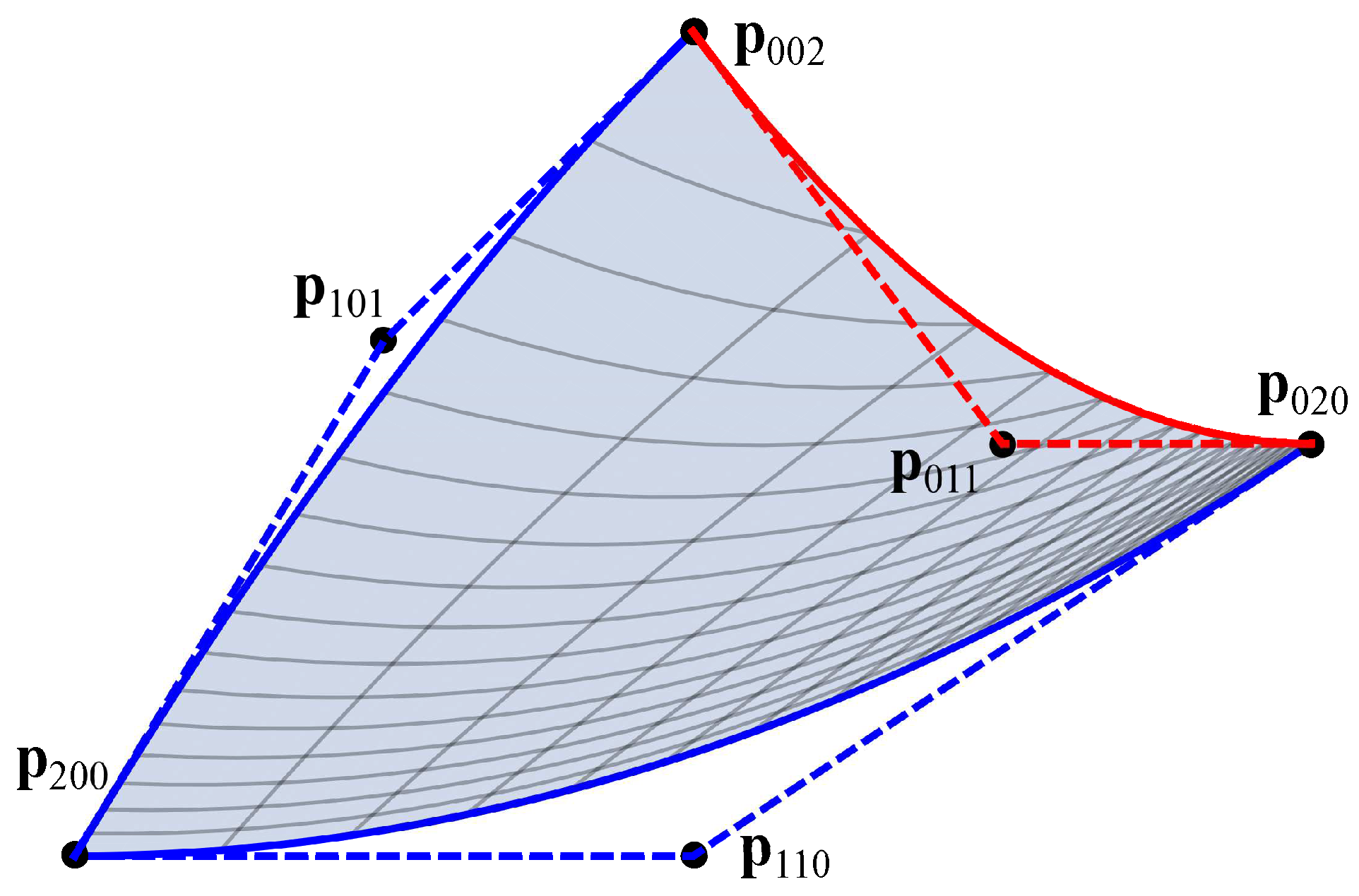
Example 4.

(${\alpha }^2=1$) Fix three endpoints ${\mathbf{p}}_{200}=(0,0),{\mathbf{p}}_{020}=(6,2),{\mathbf{p}}_{002}=(3,4)$. Set the weights $w_{200}=36,w_{020}=35,w_{002}=8$. The control points ${\mathbf{p}}_{110},{\mathbf{p}}_{101}$ are fixed by choosing ${\lambda }_{110}=1/12,{\lambda }_{101}=1/6$, i.e.,

$$\begin{array}{ccc}& {\mathbf{p}}_{110}=& ({\mathbf{p}}_{200}+{\mathbf{p}}_{020})/2+\alpha ({\mathbf{p}}_{200}-{\mathbf{p}}_{020}){\lambda }_{110}=19/6+3\alpha /2,\hfill \\ & {\mathbf{p}}_{101}=& ({\mathbf{p}}_{200}+{\mathbf{p}}_{002})/2+\alpha ({\mathbf{p}}_{200}-{\mathbf{p}}_{002}){\lambda }_{101}=1/6+5\alpha /2).\hfill \end{array}$$

Hence

$$\begin{array}{c}\hfill w_{110}=\sqrt{\frac{w_{200}{w}_{020}}{1-4{\alpha }^2{\lambda }_{110}^2}}=36,w_{101}=\sqrt{\frac{w_{200}{w}_{002}}{1-4{\alpha }^2{\lambda }_{101}^2}}=18.\end{array}$$

From (12), we obtain

$$\begin{array}{ccc}& {\mathbf{z}}_{010}=& \left(w_{110}+\alpha \sqrt{\left({\left(w_{110}\right)}^2-w_{200}{w}_{020}\right){\alpha }^2}\right)/w_{200}=1+\alpha /6,\hfill \\ & {\mathbf{z}}_{001}=& \left(w_{101}+\alpha \sqrt{\left({\left(w_{101}\right)}^2-w_{200}{w}_{002}\right){\alpha }^2}\right)/w_{200}=1/2+\alpha /6.\hfill \end{array}$$

Choose ${\mathbf{w}}_{100}=6+0\alpha$. Hence, from (11),

$$\begin{array}{ccc}& {\mathbf{w}}_{010}={\mathbf{w}}_{100}{\mathbf{z}}_{010}=6+\alpha ,& \\ & {\mathbf{w}}_{001}={\mathbf{w}}_{100}{\mathbf{z}}_{001}=3+\alpha .\end{array}$$

Set ${\mathbf{p}}_{100}={\mathbf{p}}_{200},{\mathbf{p}}_{010}={\mathbf{p}}_{020},{\mathbf{p}}_{001}={\mathbf{p}}_{002}$. $w_{011}$ and ${\mathbf{p}}_{011}$ can be calculated as follows:

$$\begin{array}{ccc}& w_{011}& =({\mathbf{w}}_{010}\overline{{\mathbf{w}}_{001}}+{\mathbf{w}}_{010}\overline{{\mathbf{w}}_{001}})/2,=17,\hfill \\ & {\mathbf{p}}_{011}& =({\mathbf{w}}_{010}\overline{{\mathbf{w}}_{001}}{\mathbf{p}}_{010}+{\mathbf{w}}_{001}\overline{{\mathbf{w}}_{010}}{\mathbf{p}}_{001})/\left(2w_{011}\right)=159/34+93\alpha /34.\hfill \end{array}$$

Thus, we obtain a rational quadratic map $\mathbf{p}(s,t)$ with complex rational representation

$${\mathbf{p}}_l(s,t)=\frac{{\mathbf{p}}_{100}{\mathbf{w}}_{100}u+{\mathbf{p}}_{010}{\mathbf{w}}_{010}s+{\mathbf{p}}_{001}{\mathbf{w}}_{001}t}{{\mathbf{w}}_{100}u+{\mathbf{w}}_{010}s+{\mathbf{w}}_{001}t}=\frac{(38s+13t)+(18s+15t)\alpha }{(6-3t)+(s+t)\alpha }.$$

See Figure 2 for an illustration of the birational map $\mathbf{p}(s,t)$.

Figure 2. A birational quadratic planar map (${\alpha }^2=1$). The points ${\mathbf{p}}_{011}$ on the red line segments are fixed when the points ${\mathbf{p}}_{101},{\mathbf{p}}_{110}$ on the blue line segments are chosen.

Let $n_0(s,t)=38s+13t$, $n_1(s,t)=18s+15t$, $d_0(s,t)=6-3t$, $d_1(s,t)=s+t$. Solving the system of equations

$$\begin{array}{c}\hfill \left\{\begin{array}{c}{l}_0(x,y;s,t)=d_0(s,t)x+{\alpha }^2{d}_1(s,t)y-n_0(s,t)=0,\hfill \\ l_1(x,y;s,t)=d_1(s,t)x+d_0(s,t)y-n_1(s,t)=0,\hfill \end{array}\right.\end{array}$$

with respect to the variables $s,t$, we obtain the inversion equation:

$$\begin{array}{c}\hfill s=-\frac{6\left(x^2-15x-y^2+13y\right)}{3x^2-79x-3y^2+117y+336},t=\frac{6\left(x^2-18x-y^2+38y\right)}{3x^2-79x-3y^2+117y+336}.\end{array}$$

Example 5.

(${\alpha }^2=0$) Fix three endpoints ${\mathbf{p}}_{200}=(0,0),{\mathbf{p}}_{020}=(6,2),{\mathbf{p}}_{002}=(3,4)$. Set the weights $w_{200}=9,w_{020}=36,w_{002}=1$. The control points ${\mathbf{p}}_{110},{\mathbf{p}}_{101}$ are fixed by choosing ${\lambda }_{110}=-1/6,{\lambda }_{101}=1/6$, i.e.,

$$\begin{array}{ccc}& {\mathbf{p}}_{110}=& ({\mathbf{p}}_{200}+{\mathbf{p}}_{020})/2+\alpha ({\mathbf{p}}_{200}-{\mathbf{p}}_{020}){\lambda }_{110}=3+0\alpha ,\hfill \\ & {\mathbf{p}}_{101}=& ({\mathbf{p}}_{200}+{\mathbf{p}}_{002})/2+\alpha ({\mathbf{p}}_{200}-{\mathbf{p}}_{002}){\lambda }_{101}=3/2+5\alpha /2.\hfill \end{array}$$

Hence

$$\begin{array}{c}\hfill w_{110}=\sqrt{\frac{w_{200}{w}_{020}}{1-4{\alpha }^2{\lambda }_{110}^2}}=18,w_{101}=\sqrt{\frac{w_{200}{w}_{002}}{1-4{\alpha }^2{\lambda }_{101}^2}}=3.\end{array}$$

From (12), we obtain

$$\begin{array}{ccc}& {\mathbf{z}}_{010}=& w_{110}\left(1+2\alpha {\lambda }_{110}\right)/w_{200}=2-2\alpha /3,\hfill \\ & {\mathbf{z}}_{001}=& w_{101}\left(1+2\alpha {\lambda }_{101}\right)/w_{200}=1/3+\alpha /9.\hfill \end{array}$$

Choose ${\mathbf{w}}_{100}=6+0\alpha$. Hence, from (11),

$$\begin{array}{ccc}& {\mathbf{w}}_{010}={\mathbf{w}}_{100}{\mathbf{z}}_{010}=6+2\alpha ,& \\ & {\mathbf{w}}_{001}={\mathbf{w}}_{100}{\mathbf{z}}_{001}=1+\alpha .\end{array}$$

Set ${\mathbf{p}}_{100}={\mathbf{p}}_{200},{\mathbf{p}}_{010}={\mathbf{p}}_{020},{\mathbf{p}}_{001}={\mathbf{p}}_{002}$. $w_{011}$ and ${\mathbf{p}}_{011}$ can be calculated as follows:

$$\begin{array}{ccc}& w_{011}=& ({\mathbf{w}}_{010}\overline{{\mathbf{w}}_{001}}+{\mathbf{w}}_{010}\overline{{\mathbf{w}}_{001}})/2=6,\hfill \\ & {\mathbf{p}}_{011}=& ({\mathbf{w}}_{010}\overline{{\mathbf{w}}_{001}}{\mathbf{p}}_{010}+{\mathbf{w}}_{001}\overline{{\mathbf{w}}_{010}}{\mathbf{p}}_{001})/\left(2w_{011}\right)=9/2+2\alpha .\hfill \end{array}$$

Thus, we obtain a rational quadratic map $\mathbf{p}(s,t)$ with complex rational representation

$$\begin{array}{c}\hfill {\mathbf{p}}_l(s,t)=\frac{{\mathbf{p}}_{100}{\mathbf{w}}_{100}u+{\mathbf{p}}_{010}{\mathbf{w}}_{010}s+{\mathbf{p}}_{001}{\mathbf{w}}_{001}t}{{\mathbf{w}}_{100}u+{\mathbf{w}}_{010}s+{\mathbf{w}}_{001}t}=\frac{(36s+3t)+(24s+7t)\alpha }{(3+3s-2t)+(2-t)\alpha }.\end{array}$$

See Figure 3 for an illustration of the birational map $\mathbf{p}(s,t)$.

Figure 3. A birational quadratic planar map (${\alpha }^2=0$). The points ${\mathbf{p}}_{011}$ on the red line segments are fixed when the points ${\mathbf{p}}_{101},{\mathbf{p}}_{110}$ on the blue line segments are chosen.

Let $n_0(s,t)=36s+3t$, $n_1(s,t)=24s+7t$, $d_0(s,t)=3+3s-2t$, $d_1(s,t)=2-t$, solving the system of equations

$$\begin{array}{c}\hfill \left\{\begin{array}{c}{l}_0(x,y;s,t)=d_0(s,t)x+{\alpha }^2{d}_1(s,t)y-n_0(s,t)=0,\hfill \\ l_1(x,y;s,t)=d_1(s,t)x+d_0(s,t)y-n_1(s,t)=0,\hfill \end{array}\right.\end{array}$$

and with respect to the variables $s,t$, we obtain the inversion equation:

$$\begin{array}{c}\hfill s=-\frac{-x^2+15x-9y}{3\left(x^2+11x-27y-60\right)},t=\frac{2\left(x^2-18y\right)}{x^2+11x-27y-60}.\end{array}$$

5. Conclusions

We extended the construction of birational quadratic maps based on rational maps over generalized complex numbers. When we need to construct birational quadratic maps, the new method provides more options for choosing the middle control points and their corresponding weights. Hence, we increase the flexibility of the boundary curves of birational quadratic maps. The proof of the birational property is based on the construction of two special syzygies. The formulas for the inversion equation are also provided. Although we have generalized the construction of birational maps based on generalized complex representations, the choice of the middle control points is still limited, and we cannot construct quadratic birational planar maps by moving the three middle points freely. In the future, we hope to construct general birational maps by setting ${\alpha }^2$ to the real values other than $-1,0,1$, which will be used as a shape parameter to control the shape of the boundaries.