Deep-Learning-Based Classification of Bangladeshi Medicinal Plants Using Neural Ensemble Models

Abstract

This research addresses the lack of publicly available datasets for Bangladeshi medicinal plants by presenting a comprehensive dataset comprising 5000 images of ten species collected under controlled conditions. To improve performance, several preprocessing techniques were employed, such as image selection, background removal, unsharp masking, contrast-limited adaptive histogram equalization, and morphological gradient. Then, we applied five state-of-the-art deep learning models to achieve benchmark performance on the dataset: VGG16, ResNet50, DenseNet201, InceptionV3, and Xception. Among these models, DenseNet201 demonstrated the highest accuracy of 85.28%. In addition to benchmarking the deep learning models, three novel neural network architectures were developed: dense-residual–dense (DRD), dense-residual–ConvLSTM-dense (DRCD), and inception-residual–ConvLSTM-dense (IRCD). The DRCD model achieved the highest accuracy of 97%, surpassing the benchmark performances of individual models. This highlights the effectiveness of the proposed architectures in capturing complex patterns and dependencies within the data. To further enhance classification accuracy, an ensemble approach was adopted, employing both hard ensemble and soft ensemble techniques. The hard ensemble achieved an accuracy of 98%, while the soft ensemble achieved the highest accuracy of 99%. These results demonstrate the effectiveness of ensembling techniques in boosting overall classification performance. The outcomes of this study have significant implications for the accurate identification and classification of Bangladeshi medicinal plants. This research provides valuable resources for traditional medicine, drug discovery, and biodiversity conservation efforts. The developed models and ensemble techniques can aid researchers, botanists, and practitioners in accurately identifying medicinal plant species, thereby facilitating the utilization of their therapeutic potential and contributing to the preservation of biodiversity.

1. Introduction

Plants have been utilized for their medicinal properties for centuries, with an extensive array of plant species found worldwide [1]. In Bangladesh alone, there are approximately 449 recognized medicinal plants [2]. However, accurately classifying these plants is a challenging task due to their often-similar shapes and colors, requiring significant time and expertise from botanists.

Traditional methods like support vector machines, K-nearest neighbors, and random forests have limitations in classifying medicinal plants. In contrast, convolutional neural networks (CNNs) excel at extracting high-level features [3]. Their application in plant classification has shown promising results [4].

In Bangladesh, a country with rich plant biodiversity, accurate identification of medicinal plants holds significant importance. However, the absence of a publicly available dataset specifically tailored for Bangladeshi medicinal plants poses a major challenge in achieving precise and efficient classification.

To address this gap, our research endeavors to actively collect and curate a comprehensive dataset of Bangladeshi medicinal plants. By cultivating ten representative species under controlled environmental conditions, we ensure the dataset’s diversity and relevance to the local ecosystem. This dataset serves as a valuable resource for further research and development in the field of medicinal plant classification.

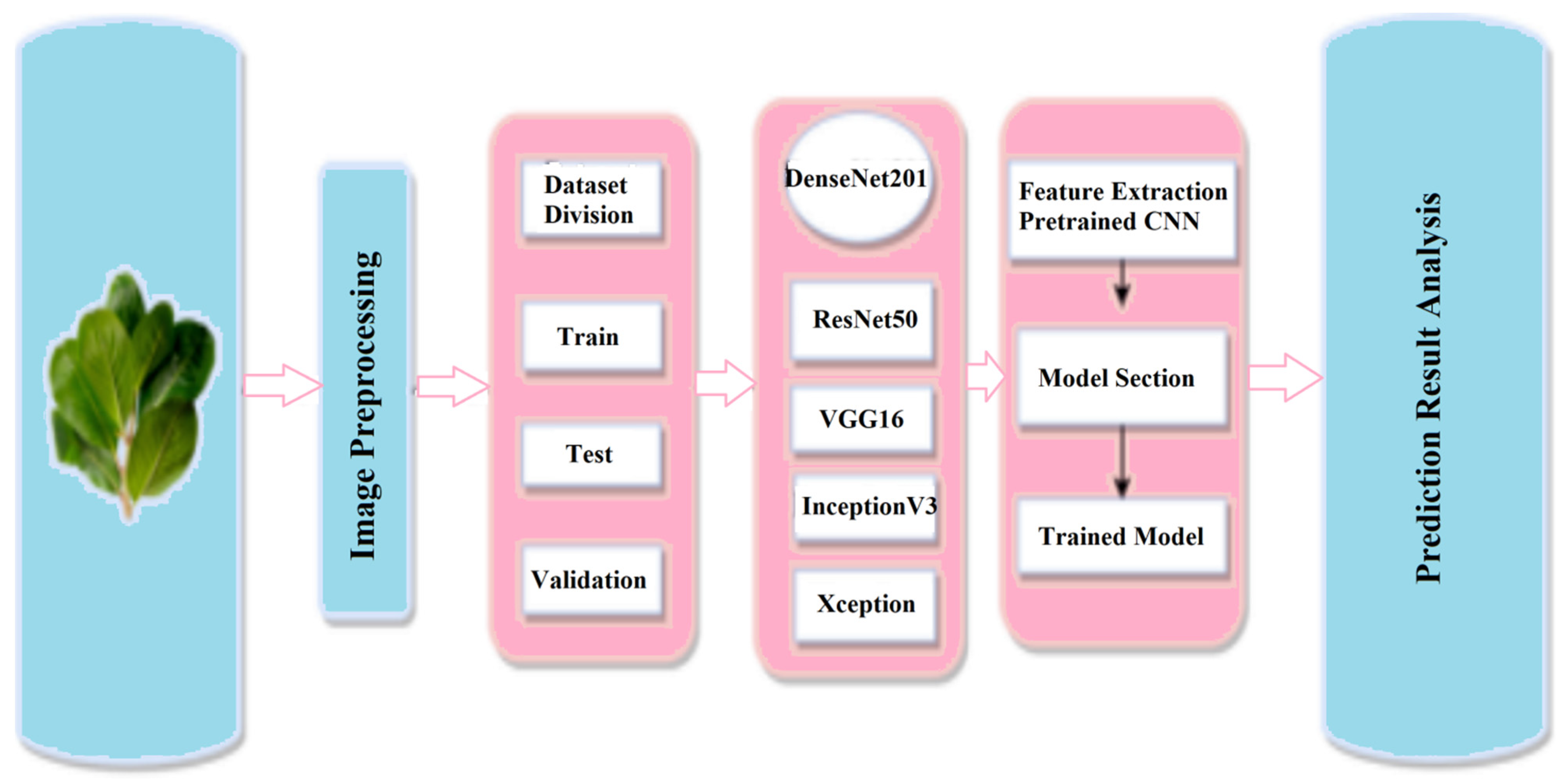
In this study, we explore the effectiveness of state-of-the-art deep learning models, namely ResNet50, VGG16, and InceptionV3, in classifying Bangladeshi medicinal plants. These models have demonstrated exceptional performance in various computer vision tasks, providing a strong foundation for our classification framework.

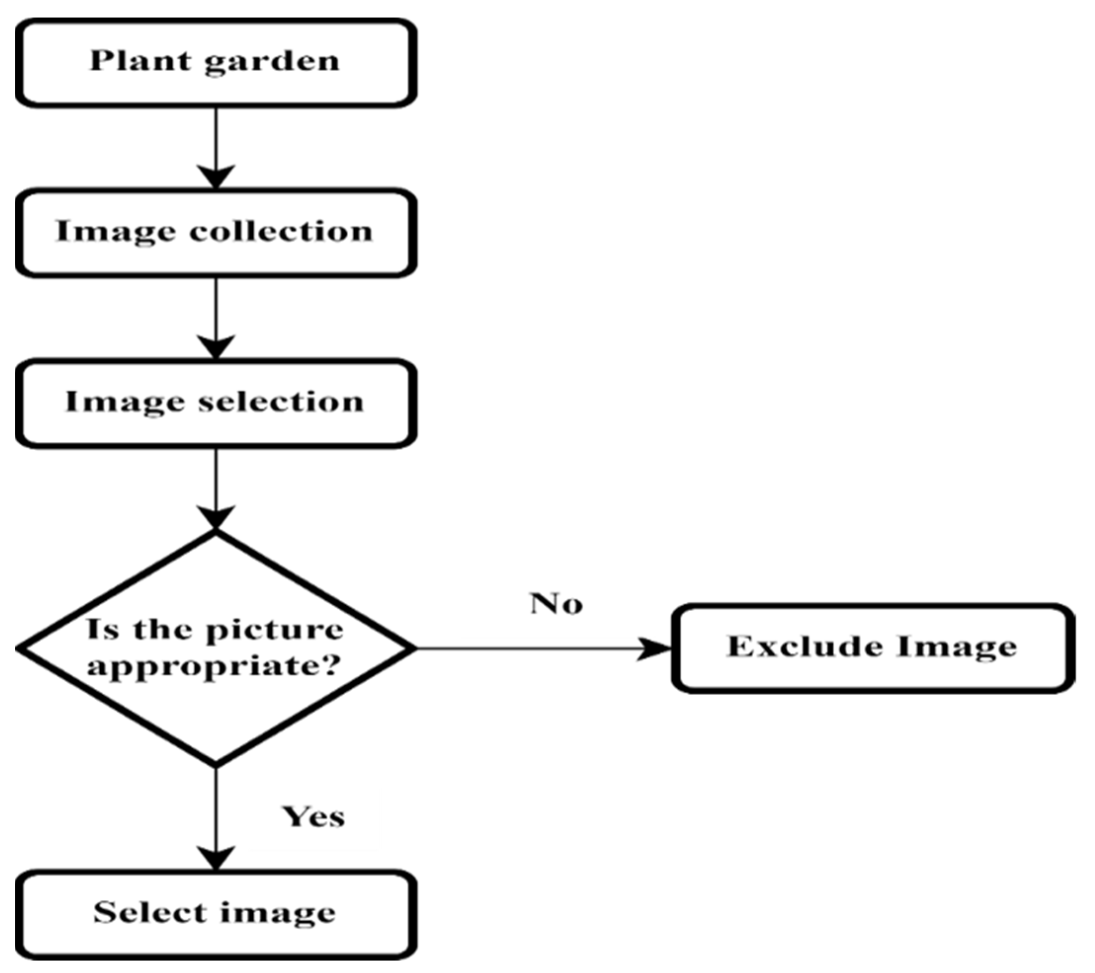
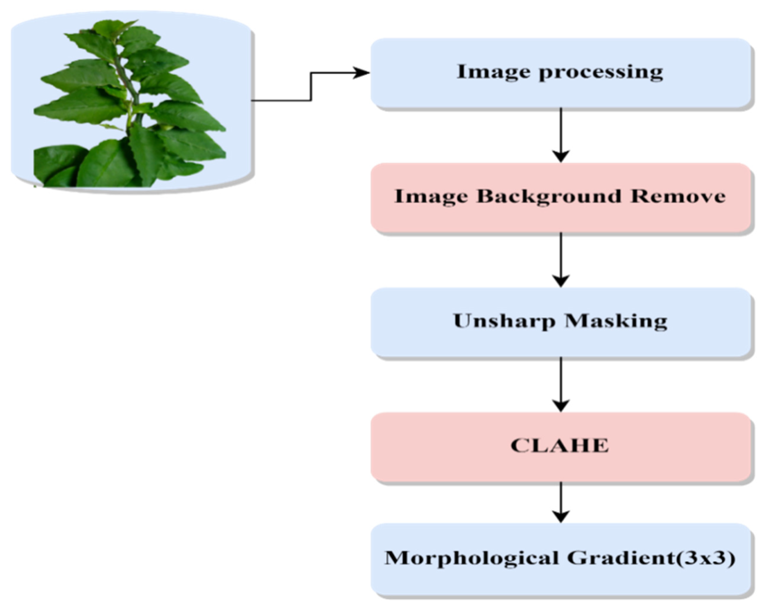
To enhance the accuracy of classification, we employ a series of preprocessing techniques. These techniques include careful image selection to ensure high-quality data, background removal to isolate plant features, unsharp masking to enhance image details, contrast-limited adaptive histogram equalization to improve image contrast, and computation of morphological gradients to highlight key plant characteristics. These preprocessing steps are crucial in optimizing the input data for the deep learning models and improving their classification performance.

Moreover, we introduce three novel neural network architectures specifically designed for medicinal plant classification: DRD, DRCD, and IRCD. These architectures incorporate unique design elements, such as dense connections, residual connections, and convolutional long-short-term memory (ConvLSTM) layers, to effectively capture spatial and temporal dependencies in the plant images.

To further enhance classification accuracy, we explore ensemble methods that combine the outputs of multiple models. By employing both hard and soft ensembling techniques, we aim to leverage the strengths of individual models and achieve superior classification performance.

Through our research, we aim to make valuable contributions to the field of medicinal plant classification in Bangladesh. These contributions include providing a curated dataset, evaluating state-of-the-art deep learning models, proposing novel neural network architectures, and showcasing the effectiveness of ensemble methods. The accurate classification of Bangladeshi medicinal plants can have a significant impact on traditional medicine practices, facilitate drug discovery efforts, and contribute to the preservation of valuable plant species.

The paper’s contributions are as follows:

• Preprocessing techniques: To enhance the quality of the images and reduce memory costs, the paper proposes and applies various preprocessing techniques to the dataset. These techniques include image selection, background removal, unsharp masking, CLAHE, and morphological gradient. These preprocessing steps improve the characteristics of the images and enhance the features relevant for classification.
• Performance evaluation of deep learning models: The paper evaluates the performance of state-of-the-art deep learning models, including VGG16, ResNet50, DenseNet201, InceptionV3, and Xception, on the Bangladeshi medicinal plant dataset. The benchmarking results provide insights into the strengths and weaknesses of these models in accurately classifying medicinal plant species. The highest accuracy achieved by DenseNet201 in our previous work [5] serves as a reference point for further improvement in this work.
• Development of neural network architectures: The paper presents three novel neural network architectures specifically designed for medicinal plant identification. The DRD, DRCD, and IRCD models are developed to capture intricate patterns and dependencies within the dataset. The DRCD model achieved the highest accuracy of 97%, surpassing the benchmark performances of individual models.
• Ensemble techniques: In order to further enhance classification accuracy, the paper applies ensemble techniques to the developed models. Both hard ensemble and soft ensemble methods are employed to combine the predictions of multiple models. The results demonstrate the effectiveness of ensemble in improving the overall classification performance, with the soft ensemble achieving the highest accuracy of 99%.
• Practical implications: The findings of this research have significant practical implications for the accurate identification and classification of Bangladeshi medicinal plants. The developed models, ensemble techniques, and comprehensive dataset contribute to the fields of traditional medicine, drug discovery, and biodiversity conservation efforts. Accurate identification of medicinal plants can aid in harnessing their therapeutic potential and preserving the rich biodiversity of Bangladesh.

The paper follows a well-structured organization, starting with Section 2, where the relevant reviews of the state-of-the-art methods are discussed. Section 3 describes the dataset preparation process in detail. In Section 4, the methodology employed for medicinal plant identification using deep learning models is presented. Section 5 then delves into the discussion of the proposed methods, providing insights into their design and implementation. The experimental results and their comprehensive discussion are covered in Section 6 and Section 7, respectively. Finally, Section 8 concludes the paper by summarizing the findings and contributions of the research while also highlighting potential future directions for further advancements in the field.

2. Review of the State of the Art

There are several significant methods for automatically classifying plants. One noteworthy study conducted by Akter and Hosen [4] focused on the classification of plant species using CNNs. They achieved a training accuracy rate of 71.3% and demonstrated the effectiveness of their approach on additional test images. S. Naeem, A. Ali, et al. [6] undertook a study on classifying medicinal plant leaves using machine learning. By employing a multi-layer perceptron classifier, they achieved an impressive accuracy of 99.01% using datasets of six types of medicinal plants.

In another study, Dahigaonkar and Kalyane [7] employed image processing techniques to identify Ayurvedic medicinal plants from leaf samples, attaining an accuracy of 96.6677% with an SVM classifier. Indrani et al. [8] developed an Android-based application that utilized the SqueezeNet CNN architecture to identify medicinal plants from their rhizomes. The application achieved a top-one accuracy of 41% and a top-five accuracy of 81% when tested on 54 rhizome sample photos.

Haryono and Sujanarko [9] compared various systems for categorizing herbal products based on leaf identification. Their CNN-based approach consistently achieved accuracy well above 90%. Anam and Saleh [10] proposed a novel method for medicinal leaf identification and authentication using a deep learning neural network. Their CNN-LSTM approach achieved an impressive accuracy rate of 94.96% in identifying nine different kinds of herbal leaves.

Pukhrambam and Rathna [11] studied the classification and identification of medicinal plants using image processing methods. They compared different models and found that GoogLeNet had a higher accuracy rate of 93%. Pudaruth et al. [12] developed the mobile application MedicPlant, which utilized deep learning techniques and a CNN model for real-time identification of medicinal plants. They achieved an accuracy of 95% using a dataset of 1000 classes with 1000 images in each class.

Zin et al. [13] explored the use of deep CNN models for herbal plant recognition, showcasing the effectiveness of these models in improving recognition accuracy, with an overall accuracy exceeding 90%. Malik et al. [14] conducted a study on automated real-time identification of medicinal plant species in the Borneo region, achieving an accuracy of 87% using deep learning models on a dataset of 2097 images from 106 species.

Jayalath et al. [15] focused on using the visual features of leaves and flowers to identify medicinal plants. They collected 5000 photos of flowers and leaves from 500 pictures of each plant, achieving a precision of 90% in identifying the flowers using their CNN-based model. Gavhale and Thakare [16] proposed a machine learning approach for medicinal plant identification using a deep neural network based on the AlexNet architecture, achieving an accuracy of 94.54% when considering form, color, and texture criteria.

Rao et al. [17] gathered a comprehensive collection of medicinal plant leaves and employed a deep learning model based on DenseNet for identification. Their model achieved an accuracy of 98% after five cross-validations. They also utilized CNN and SVM classifiers, achieving accuracies of 98% with transfer learning, 97% with SVM after hyperparameter tuning, and approximately 84% with the You Only Look Once (YOLO) algorithm.

Dileep and Pournami [18] developed the AyurLeaf model for medicinal plant categorization using deep learning techniques, achieving an accuracy of 96.76% in classifying 40 medicinal plant leaf samples. Quoc and Hoang [19] focused on using CNNs to recognize pictures of Vietnamese medicinal plants. Among the evaluated frameworks, Xception achieved the highest accuracy of 88.26%. Kan et al. [20] employed a multi-feature extraction approach and an SVM model for medicinal plant leaf image classification, attaining an accuracy of 93.3% in their study. Again, Alom et al. [5] created a new dataset of a very familiar medicinal plant, namely Brassica napus from Bangladesh. They deployed several CNN models to classify two genetically modified variations of Brassica napus from flower, packet, and leaf images. Among those models, DenseNet201 achieved the best performance, with 100% accuracy for flowers, 97% accuracy for leaves, and 100% accuracy for packet image classification.

The transformer architecture is widely used in natural language processing but has limited applications in computer vision. However, Dosovitskiy et al. [21] showed that a pure vision transformer (ViT) applied directly to image patches achieves excellent results in image classification tasks. The number of tokens impacts prediction accuracy and computational costs. To balance accuracy and speed, Wang et al. [22] developed a dynamic transformer that automatically adjusts the token number for each input image. This involves cascading multiple transformers with increasing token numbers, adaptively activating them during testing and stopping inference once a confident prediction is made. Efficient feature and relationship reuse mechanisms are also incorporated to reduce redundant computations.

3. Dataset Preparation

3.1. Data Collection

To capture the images for our dataset, we utilized a range of tools. One of the smartphones used was the Redmi Note 8, equipped with a 13-megapixel camera and a pixel density of 409 ppi (pixels per inch). Additionally, other smartphones, like the Xiaomi 7, featured an eight-megapixel camera with a pixel density of 269 ppi. The Samsung Galaxy A51 model had a 32-megapixel camera.

Figure 1 presents a flowchart illustrating the data collection process. It begins with capturing the images directly using the smartphone cameras. These images were obtained from the various types of smartphones mentioned earlier. Our dataset comprises 5000 images classified into ten different classes. The photographs were taken at specific locations, namely the Pharmacy Garden, Khwaja Yunus Ali University, and Khwaja Yunus Ali Medical College and Hospital, situated in Sirajganj, Bangladesh. In Figure 2, we provide one sample image for each of the ten species represented in the dataset.

3.2. Image Preprocessing

In the process of preparing our dataset, we conducted preprocessing steps on each raw image. Prior to including the images in the dataset, we carefully selected them by reviewing and verifying their quality. Figure 3 depicts the flowchart outlining the steps involved in data preprocessing.

3.2.1. Background Removal

During the data preprocessing stage, the background removal process was performed using the Remove Background Online tool. This tool facilitated the initial removal of the background from each image. Following that, the leaves were manually extracted from each photograph using the quick selection tools available in Adobe Photoshop CC2020. This manual extraction process ensured the precise isolation of the leaves from the remaining image elements.

To provide examples of the background removal process, Figure 4 showcases images with the background successfully removed.

In order to perform image analysis, it is common practice to extract pixel values as reference points. Once the background pixels were removed, automatic pixel counting was conducted. To gain insight into the range of pixel values, the histogram review window in Adobe Photoshop was utilized. This allowed for a visual assessment of the distribution and intensity of the remaining pixels in the image.

Furthermore, the object ratio, which indicates the proportion of the image occupied by the object of interest (in this case, the leaf), was calculated. Adobe Photoshop was employed to extract the pixel range corresponding to the object. This information helped quantify the size and scale of the leaves in relation to the entire image.

By employing a combination of automated and manual techniques using tools like Remove Background Online and Adobe Photoshop, we were able to effectively remove the background, extract relevant pixel values, and obtain essential object measurements for further analysis and classification of the medicinal plant images.

3.2.2. Unsharp Masking

Unsharp masking is a widely used image enhancement technique in digital image processing that aims to improve the sharpness and detail of an image. It operates by generating a sharpened version of the original image through the subtraction of a blurred version of the image from the original. The resulting sharpened image highlights edges and fine details, making them more visually distinct.

Mathematically, unsharp masking can be described as follows:

• Original image: Let’s $I(x,y)$ represent the original image intensity at pixel coordinates $(x,y)$.
• Blurred iage: The original image is convolved with a blur kernel to create a blurred version. This is achieved by applying a low-pass filter, such as a Gaussian filter, to reduce high-frequency components and blur the image. The blurred image is denoted as $B(x,y)$.
• Residual image: The residual image is obtained by subtracting the blurred image from the original image:

$$R\left(x,y\right)=I\left(x,y\right)-B(x,y).$$

(1)

The residual image represents the high-frequency components that were suppressed during the blurring process.

4.

Sharpened image: The sharpened image is produced by adding the residual image to the original image:

$$S\left(x,y\right)=I\left(x,y\right)+R(x,y).$$

(2)

The sharpened image enhances edges and fine details, making them more pronounced compared to the original image.

By subtracting the blurred image from the original image and then adding the resulting residual image back to the original, unsharp masking effectively enhances image sharpness and detail, leading to visually appealing and more discernible features.

3.2.3. Contrast Limited Adaptive Histogram Equalization (CLAHE)

After applying the unsharp masking technique, we further improved the characteristics of the photographs by employing contrast-limited adaptive histogram equalization (CLAHE). CLAHE is a form of adaptive histogram equalization that mitigates certain issues associated with traditional histogram equalization, such as excessive amplification of noise and artifacts. The CLAHE algorithm involves three primary components: bilinear interpolation, histogram equalization, and tile generation. Here is an overview of the steps involved:

• Image separation: The input image is divided into sections, or tiles. Each tile represents a specific portion of the image. In our case, the input image is divided into four tiles.
• Histogram equalization for each tile: Histogram equalization is performed on each tile separately using a predefined clip limit. The clip limit determines the maximum amplification that can be applied to each pixel value within the tile. The purpose of this step is to enhance the local contrast within each tile.
• Histogram computation: The histogram for each tile is computed, which involves counting the occurrences of different pixel values within the tile.
• Surplus calculation: The surplus is calculated by determining the excess pixel values that exceed the predefined clip limit.
• Excess redistribution: The excess pixel values are redistributed to the histogram bins that are under the predefined clip limit.
• Scaling and mapping using a cumulative distribution function (CDF): The histogram values are scaled and mapped using a cumulative distribution function (CDF). This step ensures that the pixel values within each tile are evenly distributed and effectively enhances the contrast.
• Tile reassembly: The generated tiles are combined using bilinear interpolation to create an output image with improved contrast. Bilinear interpolation is a method of smoothly blending neighboring pixels to create a visually seamless transition between tiles.

By applying CLAHE, we aim to enhance the contrast and improve the overall characteristics of the images. This adaptive approach considers the local characteristics of each tile, allowing for more effective contrast enhancement while avoiding excessive amplification of noise and artifacts.

3.2.4. Morphological Gradient

The morphological gradient is an image processing operation that emphasizes the boundaries or edges of objects in an image. It is computed by taking the difference between the dilation and erosion of the image using a structuring element.

If structuring element B operates image A, then the morphological gradient, G, is obtained by subtracting the eroded image from the dilated image:

$$G\left(x,y\right)=\left(A\oplus B\right)\left(x,y\right)-(A\ominus B)\left(x,y\right).$$

(3)

In other words, the morphological gradient at each pixel represents the difference between the maximum and minimum pixel values in the neighborhood defined by the structuring element. This difference highlights the boundaries or edges of objects in the image.

The choice of structuring element B determines the shape and size of the neighborhood used for computing the gradient. In this work, a 3 × 3 structuring element was applied. The size and shape of the structuring element can be customized based on the specific requirements and characteristics of the image.

By applying the morphological gradient to our dataset, we aim to emphasize the boundaries and edges of the medicinal plants, which can be useful for capturing important features and enhancing their visual representation. Figure 5 provides a visualization of the effect of applying the morphological gradient to our dataset, showcasing the highlighted boundaries and edges.

3.3. Dataset Splitting

Our dataset consists of 5000 images representing ten different species of medicinal plants. Each species is represented by 500 images, resulting in a balanced distribution of samples.

To ensure proper evaluation and training of our classification models, we partitioned the dataset into three subsets: training, testing, and validation. The split percentages we used are as follows:

Training set: We allocated 70% (3500) of the images for the training set. This subset is used to train the deep learning models and optimize their parameters. It provides the basis for the models to learn the patterns and features associated with different medicinal plant species.

Testing set: We reserved 20% (1000) of the images for the testing set. This subset is used to assess the performance and generalization ability of the trained models. It allows us to evaluate how well the models classify unseen images and estimate their accuracy based on new data.

Validation set: We set aside 10% (500) of the images for the validation set. This subset is used to fine-tune the models and optimize hyperparameters. It helps in avoiding overfitting and ensures that the selected models perform well on unseen data beyond the training and testing sets.

To ease access and coding purposes, we have uploaded the dataset to our Kaggle account. We chose the Kaggle platform due to its user-friendly interface and convenience for data management and experimentation with machine learning models. By utilizing Kaggle, we can leverage its resources and tools to conduct our classification experiments effectively.

4. Methodology

Benchmark

To establish a performance benchmark for our proposed medicinal plant species identification system, we conducted experiments using five state-of-the-art deep convolutional neural network (CNN) models: VGG16, ResNet50, DenseNet201, InceptionV3, and Xception. These models are widely recognized for their effectiveness in various computer vision tasks.

Figure 6 illustrates the benchmarking procedure we followed to evaluate the performance of these models on our dataset of medicinal plant images. The procedure can be summarized as follows:

Dataset preparation: We prepared our dataset of medicinal plant images, which includes a diverse collection of 5000 images from ten different species, with 500 images per species.

Model selection: We chose VGG16, ResNet50, DenseNet201, InceptionV3, and Xception as the benchmark models for our experiments. These models have demonstrated exceptional performance and have been extensively studied and validated in the field of computer vision.

Training and validation: We split the dataset into training, testing, and validation sets, as mentioned earlier. We used the training set to train the benchmark models, allowing them to learn the features and patterns associated with different medicinal plant species. The validation set was used to fine-tune the models and optimize their hyper-parameters.

Testing and evaluation: Once the models were trained, we evaluated their performance on the testing set. The models were presented with unseen images from the testing set, and their predictions were compared against the ground truth labels. This evaluation allowed us to assess the accuracy and performance of each benchmark model.

Performance analysis: The benchmarking procedure provided us with performance metrics such as accuracy, precision, recall, and F1 score for each benchmark model. These metrics were used to gauge the effectiveness of the models in accurately identifying medicinal plant species.

By following this benchmarking procedure, we established a baseline performance for our proposed medicinal plant species identification system using the VGG16, ResNet50, DenseNet201, InceptionV3, and Xception models. This baseline performance serves as a reference point for evaluating the effectiveness of our proposed methods and comparing their performance against state-of-the-art models.

Table 1. Classification report for the best benchmark model (DenseNet201).

	Precision	Recall	F1 Score	Support
Bohera	0.93	0.89	0.91	100
Devil backbone	0.59	0.98	0.73	100
Horitoki	0.88	0.70	0.78	100
Lemongrass	0.98	0.99	0.99	100
Nayon tara	1.00	0.32	0.48	100
Neem	0.98	0.92	0.95	100
Pathor kuchi	0.90	0.97	0.93	100
Thankuni	0.86	0.95	0.90	100
Tulsi	0.85	0.92	0.88	100
Zenora	0.85	0.88	0.87	100
Accuracy			0.85	1000
Macro average	0.88	0.85	0.84	1000
Weighted average	0.88	0.85	0.84	1000

presents the classification report for the DenseNet201 model [23], which serves as a reference point for further improvement in this work.

5. Proposed Models

5.1. Proposed Model 1: Dense-Residual–Dense (DRD)

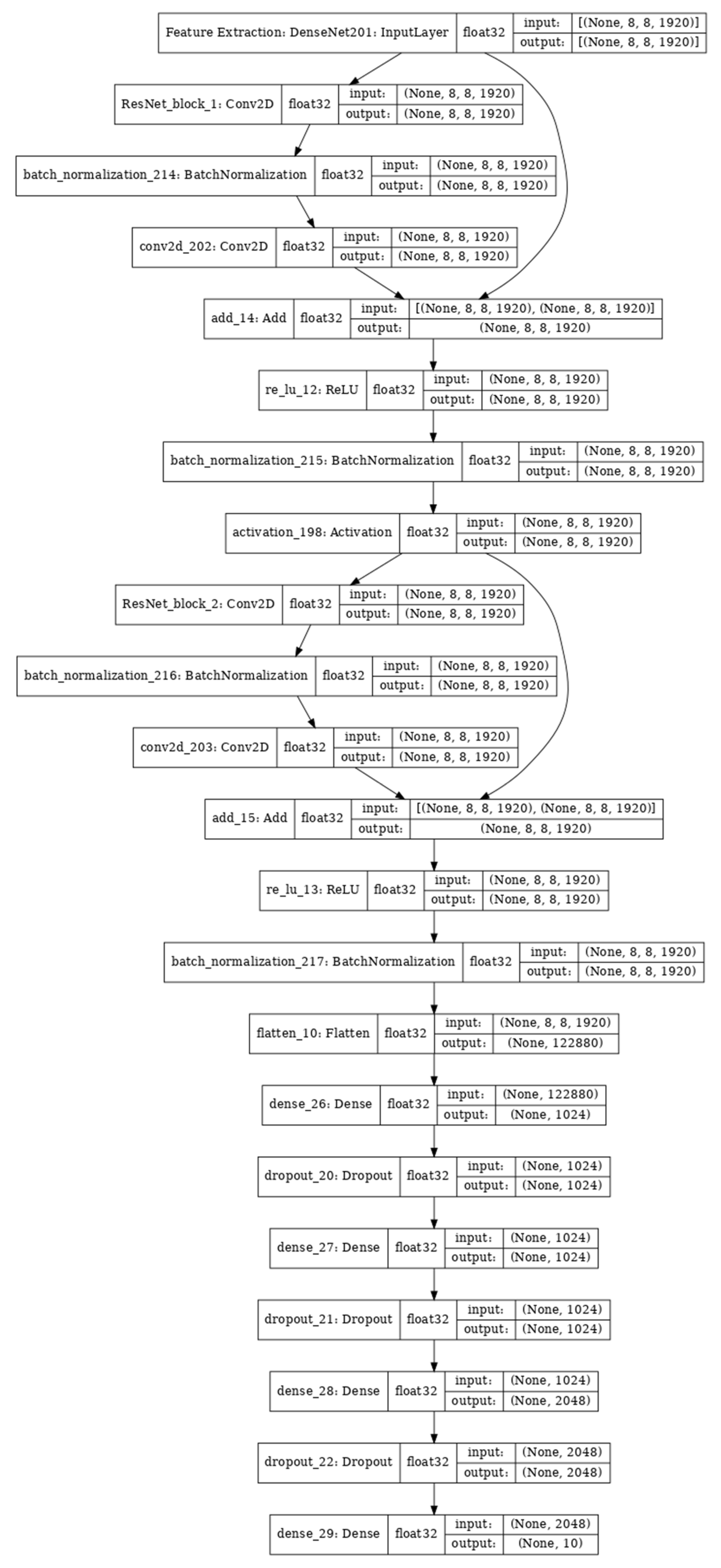
The DRD model (Figure 7) proposed in our work leverages two key components, namely dense and residual layers, to address a wide range of machine learning tasks. The model’s name reflects the sequential arrangement of these layers, which is as follows:

Dense layer: At the beginning of the DRD model, a fully connected dense layer is employed to map the input data to a higher-dimensional space. This step enables the model to capture intricate patterns and relationships within the data.

Residual connection: The residual connection, also known as a skip connection, allows information to bypass certain layers and flow directly to the output. In the DRD model, residual connections are typically introduced after each dense layer. These connections help alleviate the vanishing gradients problem, which can hinder deep network training, and improve the effectiveness of the model’s training process.

Dense layer: Following the residual connection, another fully connected dense layer is added to further transform the output from the previous layer into a higher-dimensional representation.

Output layer: The final layer of the network produces the desired output. The output can be a single value, suitable for regression tasks, or a probability distribution across multiple classes, suitable for classification tasks.

The ResNet_1 and ResNet_2 architectures, as described, showcase the specific layers and transformations applied in the model. These architectures consist of convolutional layers, transition layers, dense blocks, flattening, dropout, and an output layer. The specific dimensions, filter sizes, growth rates, and other architectural details may vary depending on the specific implementation and task requirements. For example, ResNet_1:

Input layer: accepts an input image with dimensions (8, 8, 1920).

Convolutional layer: applies a 7 × 7 convolution with 64 filters, followed by batch normalization and ReLU activation.

Transition layer 1: comprises batch normalization, 1 × 1 convolution with 256 filters, and 2 × 2 average pooling.

ResNet_2:

Input layer: accepts an input image with dimensions (8, 8, 1920).

Convolutional layer: applies a 7 × 7 convolution with 64 filters, followed by batch normalization and ReLU activation.

Transition layer 2: comprises batch normalization, 1 × 1 convolution with 512 filters, and 2 × 2 average pooling.

Transition layer 3: comprises batch normalization, 1 × 1 convolution with 1024 filters, and 2 × 2 average pooling.

Flatten: In the DenseNet-201 architecture, the final dense block produces a four-dimensional tensor, which needs to be flattened into a two-dimensional tensor before passing it to the output layer.

Dropout: To mitigate overfitting, a dropout layer with a rate of 0.5 can be included after the final dense block in the DenseNet-201 architecture.

Dense blocks:

Dense block 1: composed of 6 dense layers with a growth rate of 32.

Dense block 2: composed of 12 dense layers with a growth rate of 32.

Dense block 3: composed of 48 dense layers with a growth rate of 32.

Dense block 4: composed of 32 dense layers with a growth rate of 32.

Output layer: consists of a global average pooling layer followed by a fully connected layer.

The DRD model effectively integrates dense and residual layers in a specific order to capture complex patterns in the input data. The incorporation of residual connections helps address training challenges associated with deep networks, such as vanishing gradients. It is important to note that the exact architecture and parameters of the DRD model may vary depending on the specific task and input data characteristics.

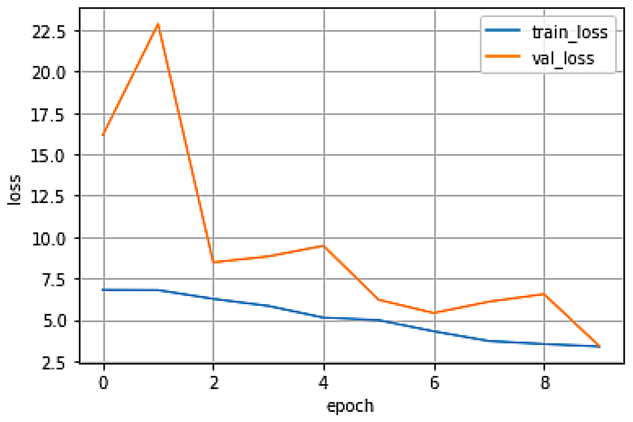
Furthermore, from Figure 8, we can observe the decreasing trend in both training loss and validation loss. This indicates that the model’s training process is progressing and that it is gradually improving its performance. Monitoring these loss values helps assess the convergence and effectiveness of the training process.

5.2. Proposed Model 2: Dense-Residual–ConvLSTM-Dense (DRCD)

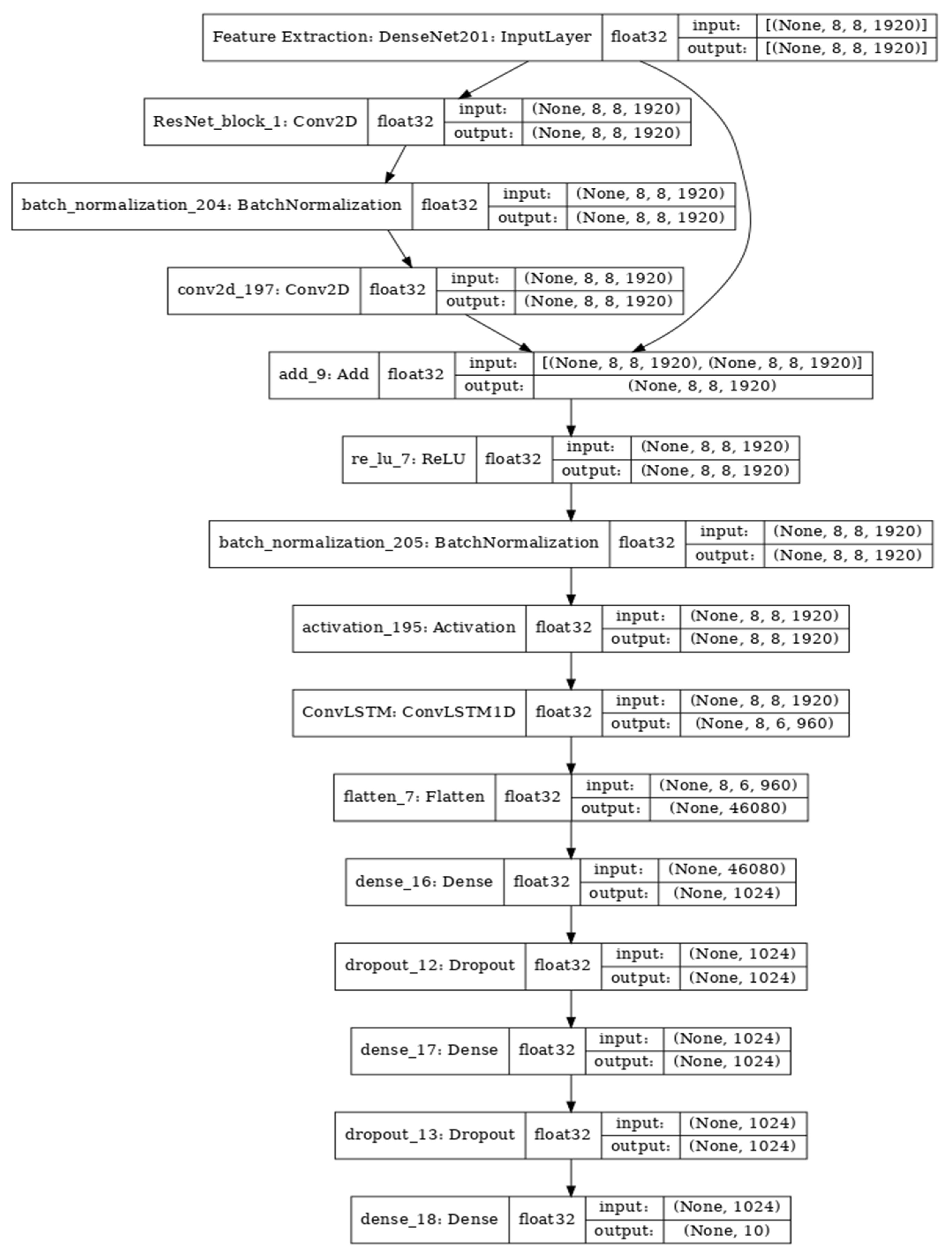
The DRCD model (Figure 9) proposed in our work is specifically designed for sequence processing tasks. It incorporates several key building blocks to effectively capture complex patterns and dependencies in sequential data. The components of the DRCD model are as follows:

Dense layer: The initial fully connected dense layer maps the input sequence to a higher-dimensional space. This step allows the model to capture intricate patterns and relationships within the sequence.

Residual connection: Residual connections are introduced after each ConvLSTM layer in the model. These connections enable the information to bypass certain layers and flow directly to the output. By incorporating residual connections, the DRCD model addresses the vanishing gradient problem and improves the effectiveness of training.

ConvLSTM layer: The ConvLSTM layer is a variant of the LSTM (long short-term memory) network that operates on sequences. It combines convolutional layers with the LSTM architecture, allowing the model to learn long-term dependencies in the input data. Each ConvLSTM layer consists of parallel convolutional layers followed by gated recurrent units (GRUs) that update the cell state and output at each time step.

Dense layer: Following the ConvLSTM layer, another fully connected dense layer is added to further transform the output into a higher-dimensional representation.

Output layer: The final layer of the network produces the desired output. For regression tasks, the output can be a single value. For classification tasks, it can be a probability distribution across multiple classes.

The DRCD model combines these layers in a specific order to capture complex patterns and dependencies in sequential data. The inclusion of residual connections helps address the issue of vanishing gradients, ensuring more effective training of the model. It is important to note that the specific architecture and parameters of the DRCD model may vary depending on the task and the characteristics of the input sequence.

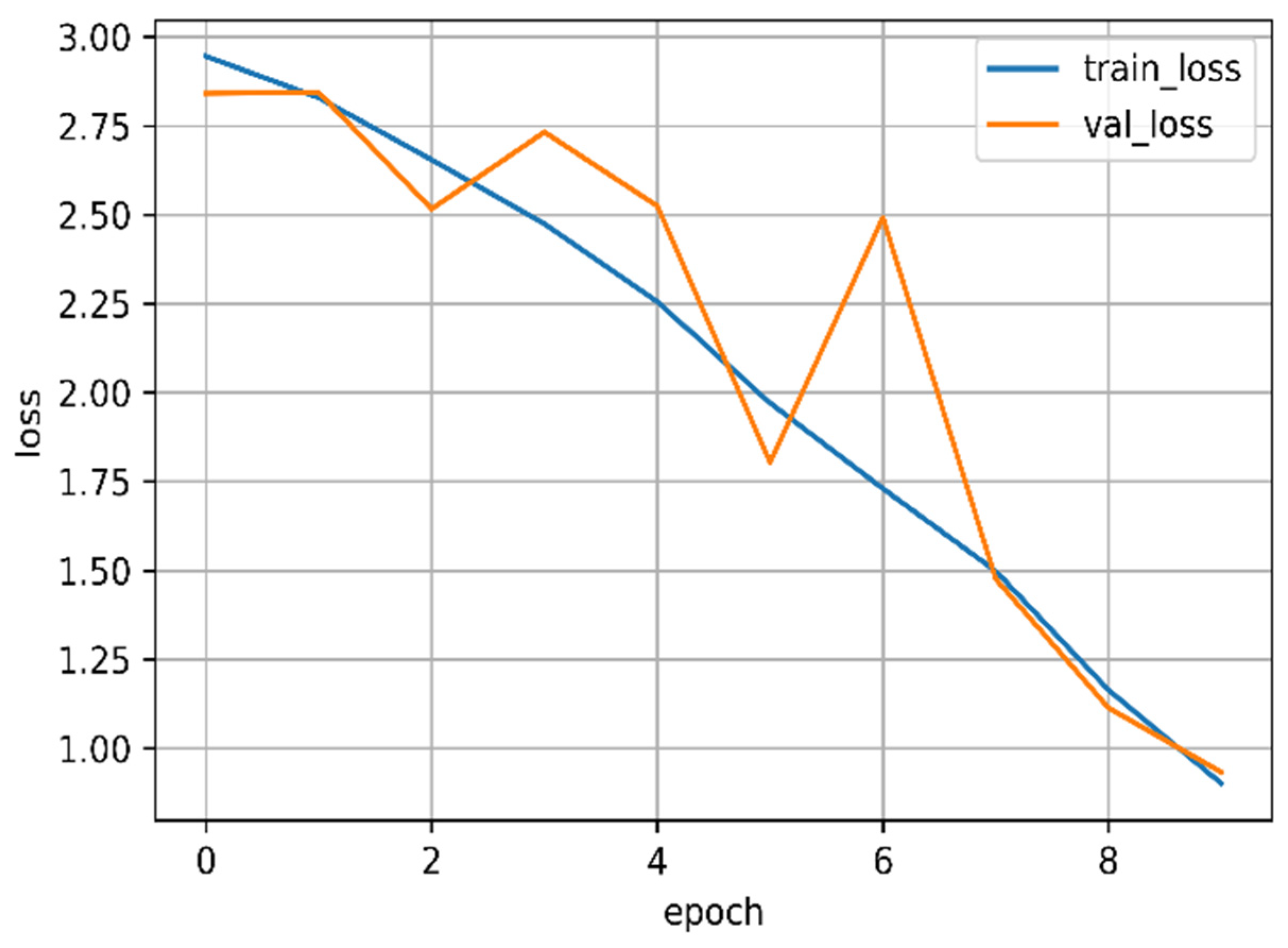
Figure 10 visualizes the learning trend of the DRCD model on the dataset, showcasing the evolution of the model’s performance during the training process. Monitoring this trend helps assess the convergence and effectiveness of the model’s training.

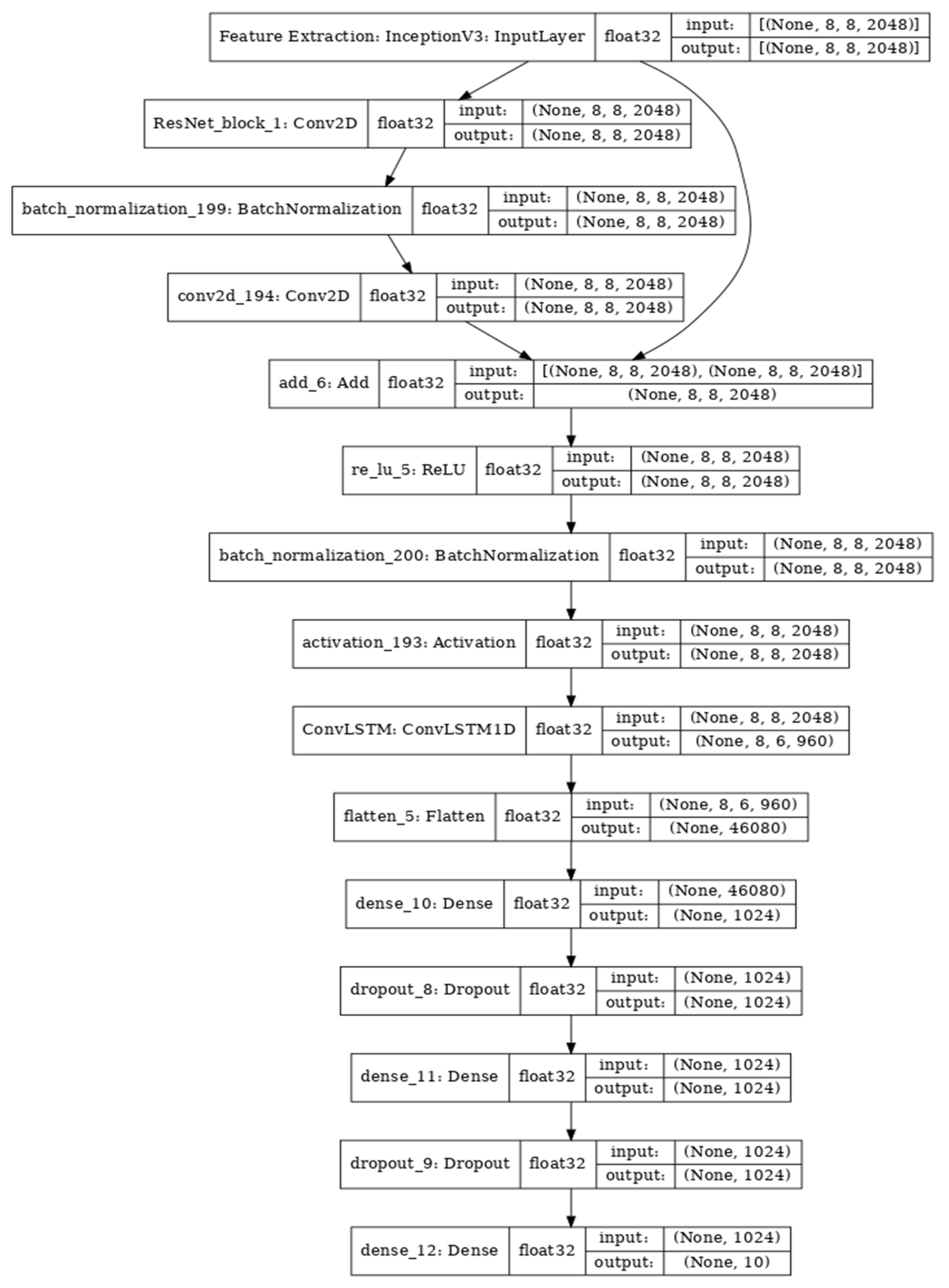
5.3. Proposed Model 3: Inception-Residual–ConvLSTM-Dense (IRCD)

The IRCD model (Figure 11) proposed in our work is designed to effectively process and extract features from input data. It incorporates several key components that work together to achieve this goal. The architecture of the IRCD model can be described as follows:

Input layer: The model begins with an input layer that takes in the input data.

Inception module: The Inception module is responsible for extracting features at multiple scales. It achieves this by performing various convolutions with different kernel sizes and pooling operations. The Inception module captures diverse information from the input, enabling the model to extract rich and multi-scale features.

Residual connection: The Inception module is connected to the subsequent layers through a residual connection. This connection allows the gradient to flow and helps address the vanishing gradient problem during training. The residual connection facilitates stable gradient flow and ensures information propagation.

ConvLSTM layer: A ConvLSTM layer is employed to process the spatial information in the input. The ConvLSTM layer combines convolutional and LSTM operations, enabling the model to capture both spatial and temporal dependencies in the data. This layer enhances the model’s ability to model temporal relationships and capture long-term dependencies.

Another residual connection: A residual connection is used to connect the ConvLSTM layer with the subsequent layers. This connection ensures stable gradient flow and facilitates the propagation of information throughout the network.

Second inception module: Another Inception module is used to further extract multi-scale features from the processed data. This module, similar to the previous one, performs various convolutional and pooling operations to capture diverse information from the input. It enhances the model’s feature extraction capabilities.

Another ConvLSTM layer: Another ConvLSTM layer is employed to process the features extracted by the second Inception module. This layer captures additional spatial information and further enhances the model’s ability to model temporal dependencies.

Another residual connection: Similar to previous layers, a residual connection is used to connect the second ConvLSTM layer with the subsequent layers. This connection ensures stable gradient flow and facilitates information propagation.

Dense layer: Finally, a dense layer is added to the architecture to map the output of the preceding layers to the desired format. The dense layer performs a linear transformation followed by a non-linear activation function to generate the final output of the model.

The output layer represents the final predictions or representations produced by the IRCD model. The combination of Inception modules, ConvLSTM layers, and residual connections allows the model to effectively process various inputs and generate meaningful predictions or representations for the given task.

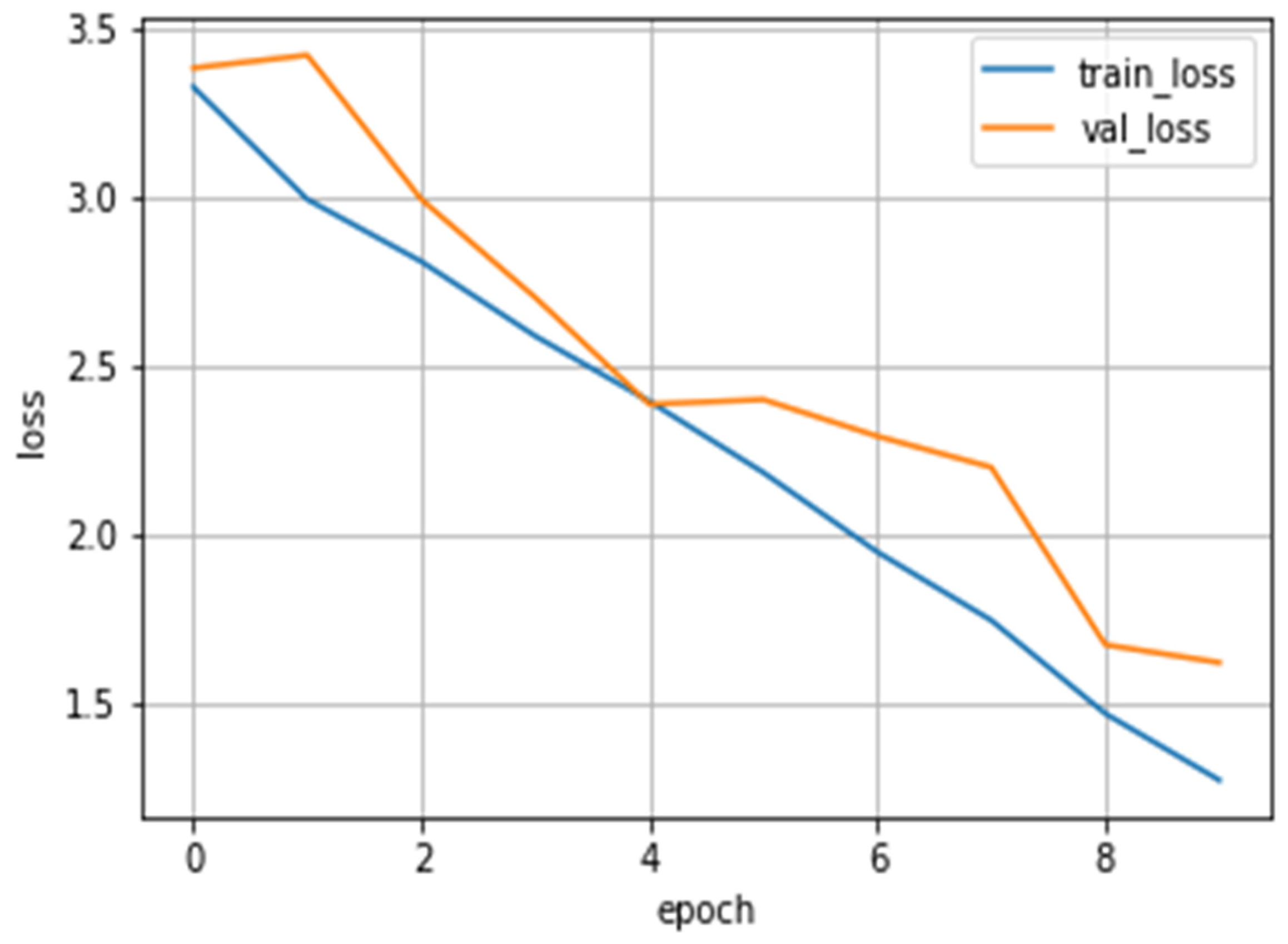
Figure 12 demonstrates the learning trend of the proposed IRCD model on the developed dataset, illustrating the evolution of the model’s performance during the training process. Monitoring this trend helps assess the convergence and effectiveness of the model’s training.

6. Result Analysis

6.1. Experimental Setup

Hyper-parameter settings play a crucial role in the training process and overall performance of each model. The batch size determines the number of samples processed in each training iteration. The image dimension and interpolation method define the size and technique used for resizing the images. The loss function measures the discrepancy between predicted and actual values. The optimizer algorithm updates the model’s parameters during training. The number of epochs specifies the total number of times the entire dataset is passed through the model. The learning rate controls the step size in parameter updates, while the learning rate decay factor reduces the learning rate over time to fine-tune the model.

While the proposed DRD, DRCD, and IRCD models share some common hyper-parameters, each model has some specific settings:

Common hyper-parameters:

• Batch size: 16
• Image dimension: 256 × 256 × 3
• Interpolation: “lanczos”
• Loss function: categorical cross-entropy
• Optimizer: RMSProp

Benchmark models’ hyper-parameters:

• Learning rate: 1 × 10⁻⁴
• Learning rate decay: 1 × 10⁻⁵
• Number of epochs: varied (benchmark models were trained until we encountered five consecutive epochs of no performance improvement on validation loss)

Proposed DRD model hyper-parameters:

• Learning rate: 1 × 10⁻⁴
• Learning rate decay: 1 × 10⁻⁵
• Number of epochs: 10

Proposed DRCD model hyper-parameters:

• Learning rate: 5 × 10⁻⁵
• Learning rate decay: 1 × 10⁻⁶
• Number of epochs: 10

Proposed IRCD model hyper-parameters:

• Learning rate: 5 × 10⁻⁵
• Learning rate decay: 1 × 10⁻⁶
• Number of epochs: 10

6.2. Evaluation Criteria

In evaluating our proposed architectures against the benchmark models, we employed several performance metrics, including accuracy, precision, recall, and F1 score. Accuracy measures the overall correctness of the predictions, indicating the percentage of correctly classified instances. Precision quantifies the proportion of correctly predicted positive instances out of all instances predicted as positive, providing insight into the model’s ability to avoid false positives. Recall, also known as sensitivity or true positive rate, measures the proportion of correctly predicted positive instances out of all actual positive instances, highlighting the model’s ability to identify true positives. F1 score combines precision and recall into a single metric, providing a balanced measure that considers both metrics equally.

6.3. Result for the Benchmark Models

For benchmarking, we applied five state-of-the-art CNN networks, namely VGG16, ResNet50, DenseNet201, InceptionV3, and Xception.

Table 2. Model performance comparison for the five state-of-the-art CNN networks.

Model	No. of Epochs	Accuracy (%)	Precision	Recall	F1 Score
VGG16	7	67	0.67	0.67	0.65
ResNet50	8	33	0.45	0.33	0.32
DenseNet201	17	85	0.88	0.85	0.84
InceptionV3	16	76	0.81	0.76	0.74
Xception	9	67	0.76	0.67	0.64

lists the performances. The accuracies (%) of these models were 67, 33, 85, 76, and 67, respectively. Again, the precisions of the networks were 0.67, 0.45, 0.88, 0.81, and 0.76, respectively. Moreover, the respective recall values were 0.67, 0.33, 0.85, 0.76, and 0.67. Finally, the F1 scores for applying the benchmark models to the dataset were 0.65, 0.32, 0.84, 0.74, and 0.64, respectively. We can clearly observe that the DenseNet201 model achieved the best performance among other benchmark models.

6.4. Result for the Proposed DRD Model

The evaluation of the DRD model resulted in high performance across multiple evaluation parameters. The model achieved an overall accuracy of 95%, indicating that it correctly classified 95% of the samples in the dataset. The precision values for each class varied, with bohera and lemongrass achieving 100% precision, indicating that all the predicted instances for these classes were correct. Other classes also demonstrated high precision values ranging from 81% to 100%.

The recall values indicate the model’s ability to correctly identify instances of each class. Devil backbone, lemongrass, nayon tara, neem, and tulsi achieved perfect recall scores of 100%, indicating that the model successfully identified all instances of these classes. Other classes showed recall values ranging from 79% to 100%.

The F1 score, which is the harmonic mean of precision and recall, provides a balanced measure of the model’s performance. The DRD model obtained high F1 scores for most classes, ranging from 88% to 100%. Devil backbone, lemongrass, and bohera achieved particularly high F1 scores of 99% or above.

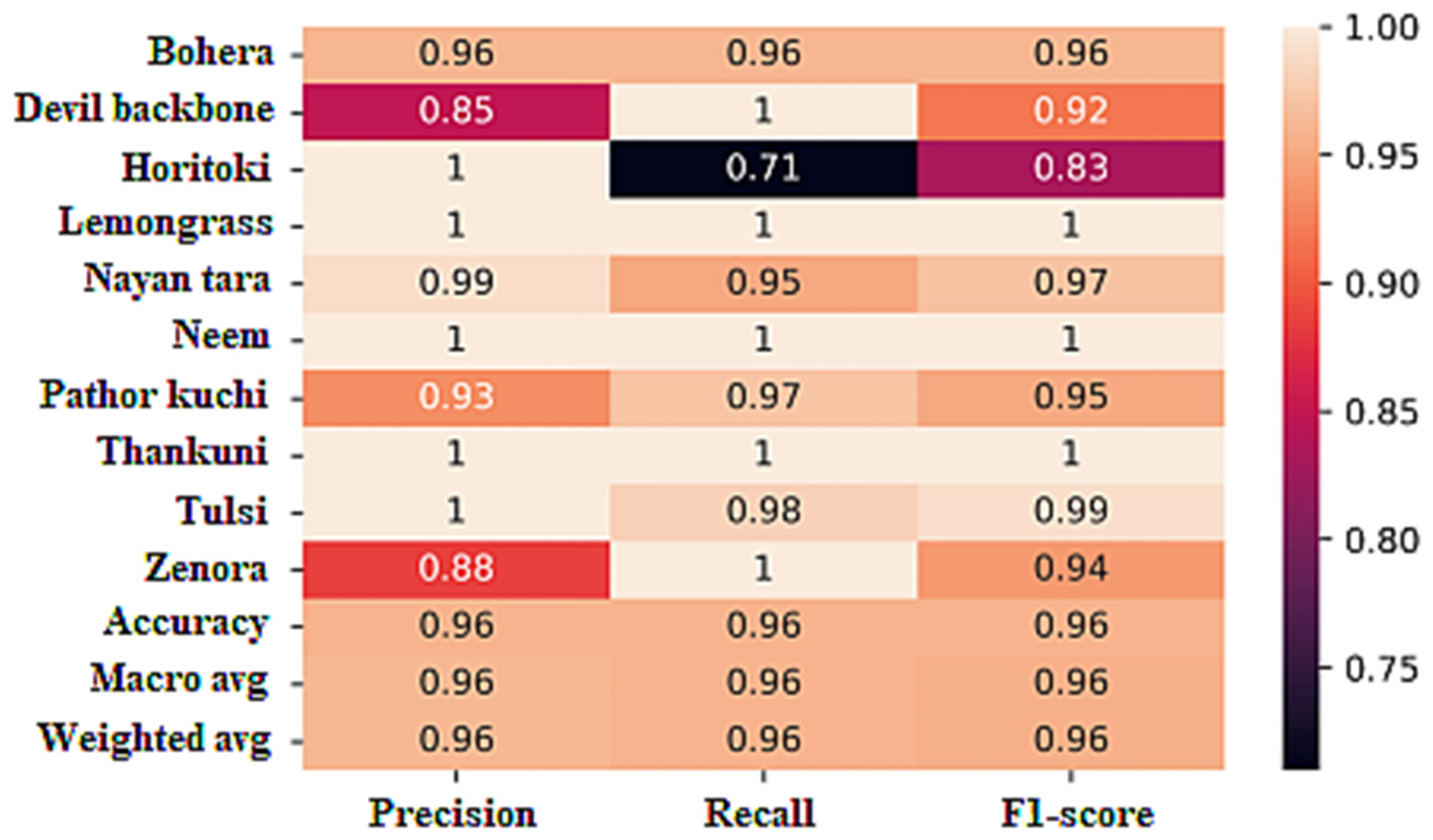
Overall, the DRD model demonstrated strong performance with accuracy, precision, recall, and F1 score values of 95%. These results indicate the model’s effectiveness in accurately classifying the medicinal plant species in the dataset. The classification report in Figure 13 provides detailed statistics for each class, showcasing the model’s performance across different evaluation metrics.

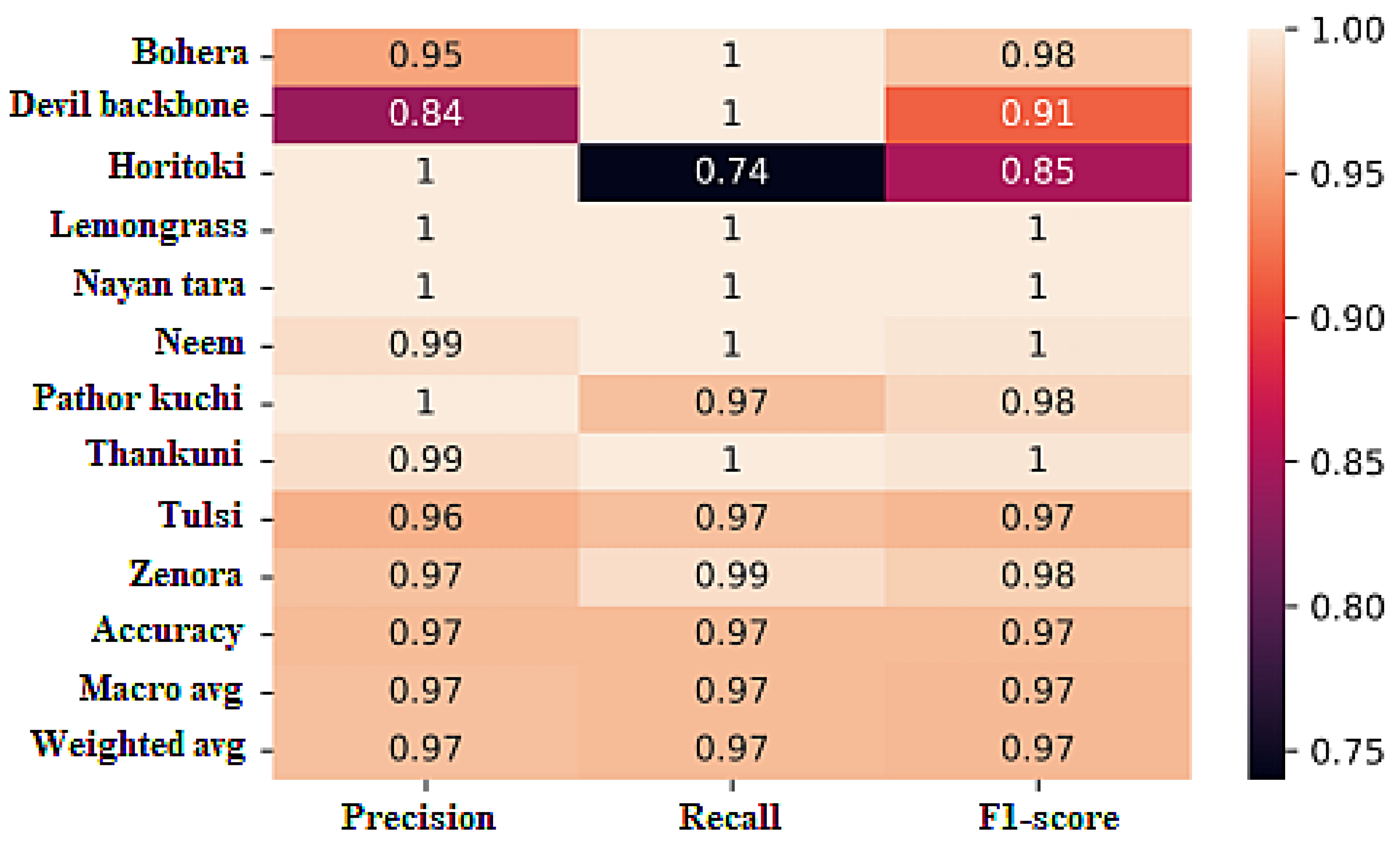
6.5. Result for the Proposed DRCD Model

The classification report of the DRCD model, as shown in Figure 14, reveals the model’s performance across different evaluation metrics for each class.

For the class bohera, the DRCD model achieved a precision of 95%, indicating that 95% of the predicted instances for this class were correct. The recall value of 100% indicates that the model correctly identified all instances of bohera. The F1 score, which is the harmonic mean of precision and recall, was calculated to be 98%, reflecting the overall performance of the model for this class.

Similarly, for devil backbone, the model achieved 84% precision, meaning that 84% of the predicted instances for this class were correct. The recall value of 100% indicates that all instances of devil backbone were correctly identified by the model. The F1 score, which takes into account both precision and recall, was calculated to be 91%, representing the overall performance of the model for this class.

For other classes, such as horitoki, lemongrass, nayon tara, neem, pathor kuchi, thankuni, tulsi, and zenora, the DRCD model demonstrated high precision, recall, and F1 scores, ranging from 74% to 100%. These scores indicate the model’s ability to accurately classify instances of these classes.

The overall accuracy of the DRCD model was 97%, reflecting the percentage of correctly classified instances across all classes. The overall precision, recall, and F1 scores were also 97%, indicating the model’s balanced performance across the entire dataset.

These evaluation metrics highlight the effectiveness of the DRCD model in accurately classifying the medicinal plant species in the dataset, with high precision, recall, and F1 scores, resulting in an overall accuracy of 97%.

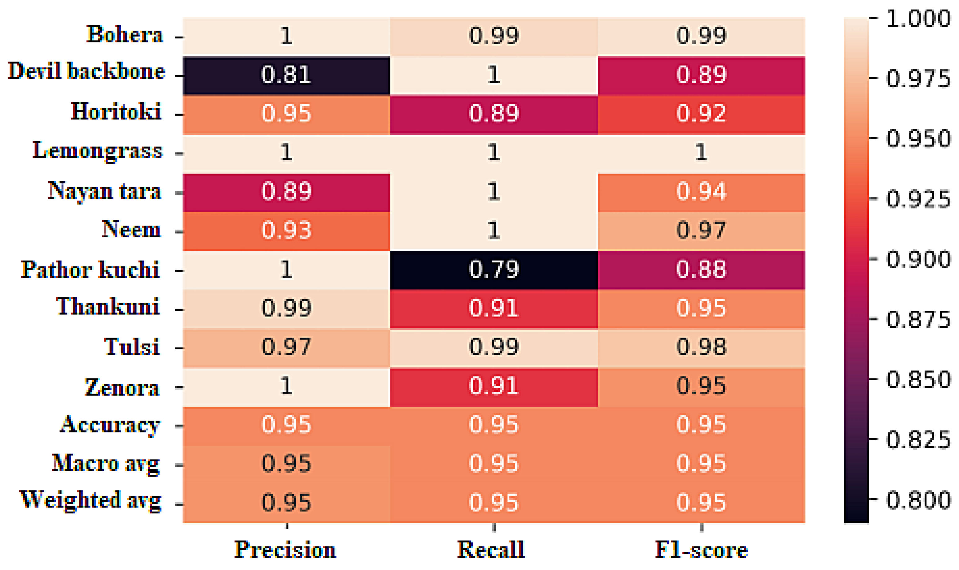
6.6. Result for the Proposed IRCD Model

The classification report for the IRCD model, as presented in Figure 15, provides an overview of its performance across different evaluation metrics for each class.

For the class bohera, the IRCD model achieved a precision of 96%, indicating that 96% of the predicted instances for this class were correct. The recall value of 96% indicates that the model correctly identified 96% of the instances of bohera. The F1 score, which is the harmonic mean of precision and recall, was calculated to be 96%, representing the overall performance of the model for this class.

For devil backbone, the model achieved a precision of 80%, indicating that 80% of the predicted instances for this class were correct. The recall value of 100% suggests that all instances of devil backbone were correctly identified by the model. The F1 score, combining precision and recall, was calculated to be 92%, reflecting the overall performance of the model for this class.

Similar evaluations were carried out for other classes, including horitoki, lemongrass, nayon tara, neem, pathor kuchi, thankuni, tulsi, and zenora. The model demonstrated high precision, recall, and F1 scores for most classes, ranging from 71% to 100%. These scores indicate the model’s ability to accurately classify instances of these classes.

The overall accuracy of the IRCD model on the dataset was 96%, indicating the percentage of correctly classified instances across all classes. The overall precision, recall, and F1 scores were also 96%, demonstrating the model’s balanced performance across the entire dataset.

In summary, the IRCD model achieved an accuracy, precision, recall, and F1 score of 96% on the dataset, showcasing its effectiveness in accurately classifying the medicinal plant species.

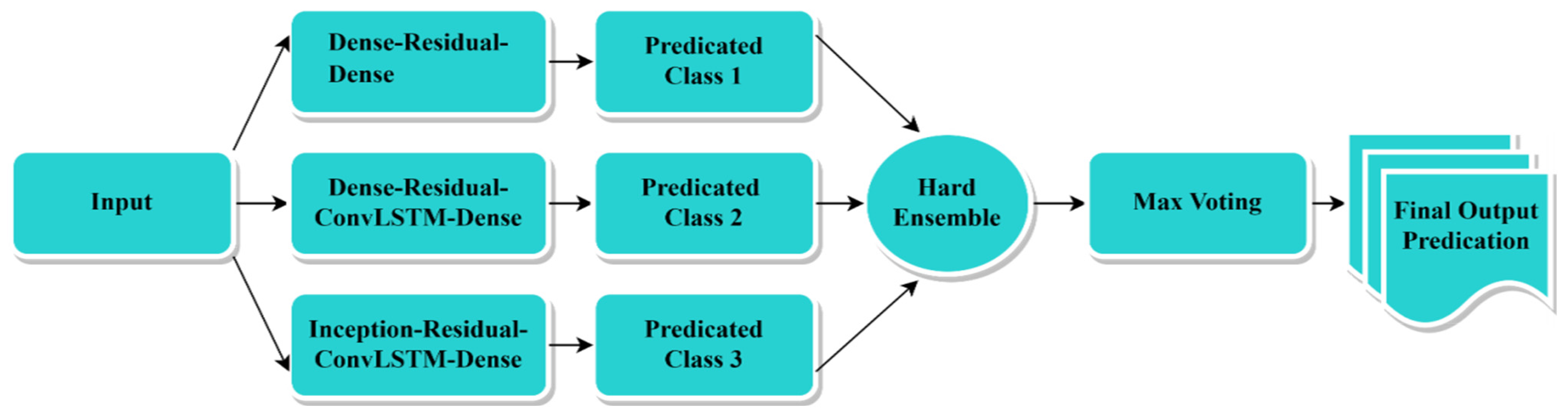
6.7. Result for the Proposed Model Using Hard Ensemble

The hard ensemble, which combines the predictions of multiple models through majority voting, achieved promising results on the dataset. Figure 16 depicts the procedure for applying hard ensemble to our proposed models. The classification report and confusion matrix statistics in Figure 17 and Figure 18 provide a comprehensive evaluation of the hard ensemble’s performance.

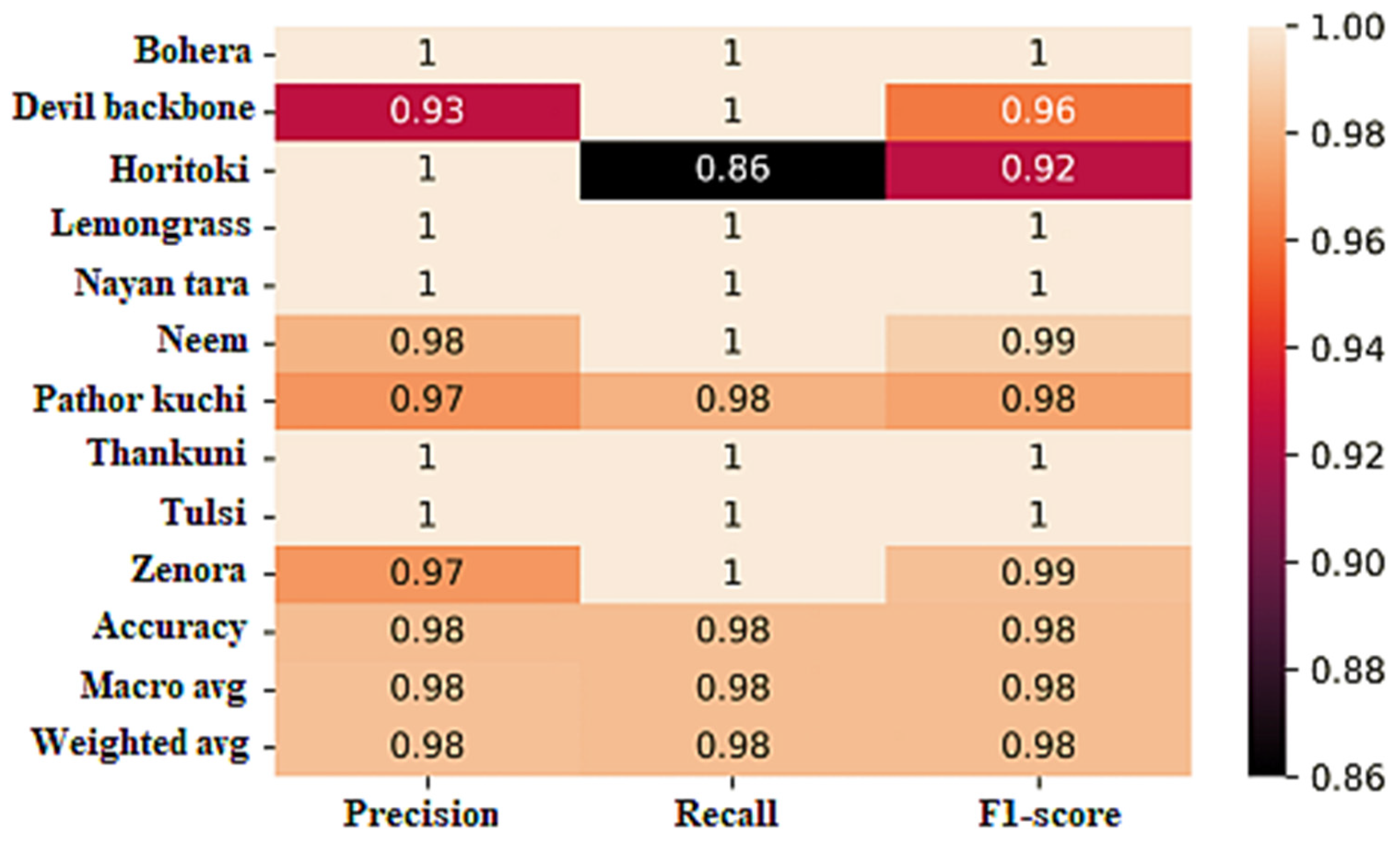
For each class, the hard ensemble achieved high precision, recall, and F1 scores. Notably, it achieved an accuracy of 98%, indicating that the ensemble accurately classified 98% of the instances in the dataset.

Specifically, the hard ensemble obtained a precision of 100%, a recall of 100%, and an F1 score of 100% for the bohera class. This indicates that the ensemble effectively identified instances of bohera with high precision and recall.

For devil backbone, the hard ensemble achieved 93% precision, 100% recall, and a 96% F1 score. Similarly, for horitoki, it achieved 100% precision, 86% recall, and a 92% F1 score. These results demonstrate the ensemble’s ability to accurately classify instances of these classes.

The hard ensemble achieved perfect precision, recall, and F1 scores (100%) for the classes lemongrass, nayon tara, thankuni, and tulsi, indicating flawless classification performance for these classes.

Overall, the hard ensemble exhibited strong performance across all evaluation metrics, with accuracy, precision, recall, and F1 scores of 98%. This indicates its effectiveness in accurately classifying medicinal plant species.

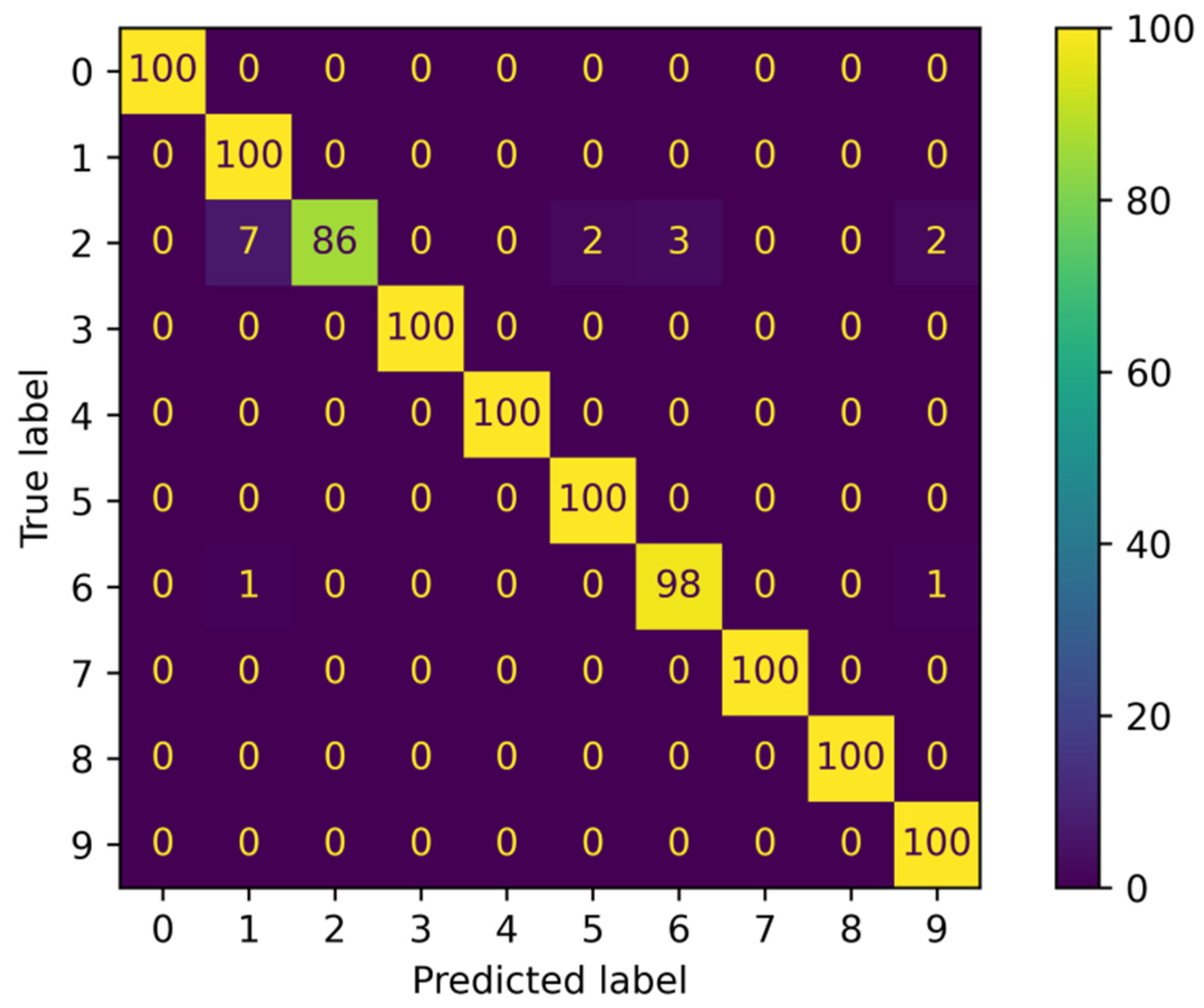
The confusion matrix in Figure 18 provides additional insights into the ensemble’s performance. It illustrates the number of instances that were correctly classified and misclassified for each class. The high values along the diagonal of the confusion matrix indicate that the majority of instances were correctly classified by the ensemble.

In summary, the hard ensemble of our proposed neural models achieved an impressive accuracy of 98%, along with high precision, recall, and F1 scores for each class. These results demonstrate the effectiveness of ensemble learning in improving the overall performance of the models.

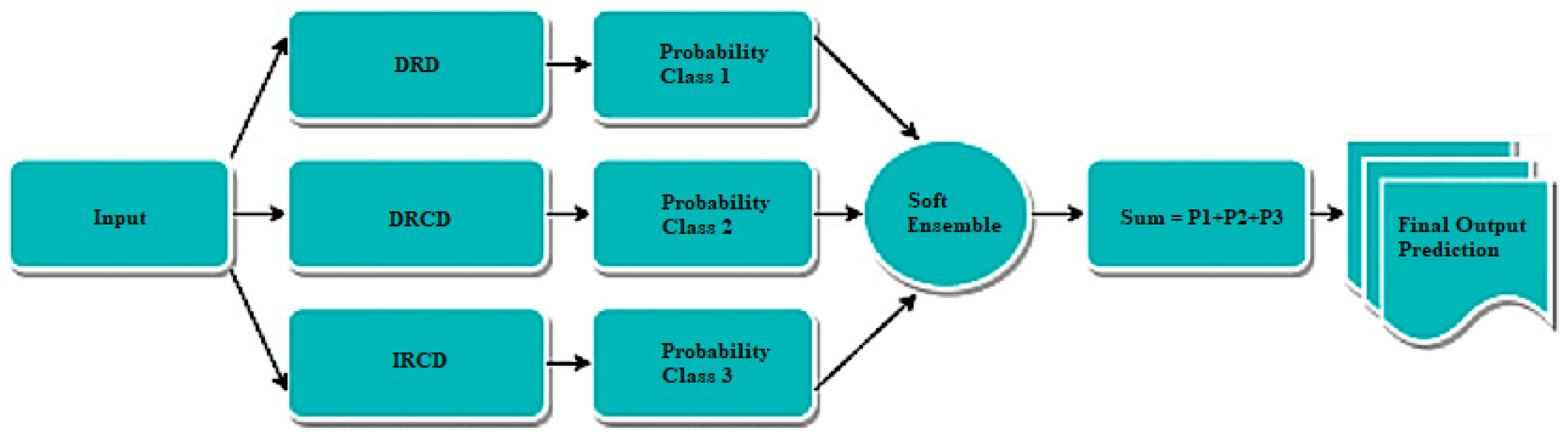
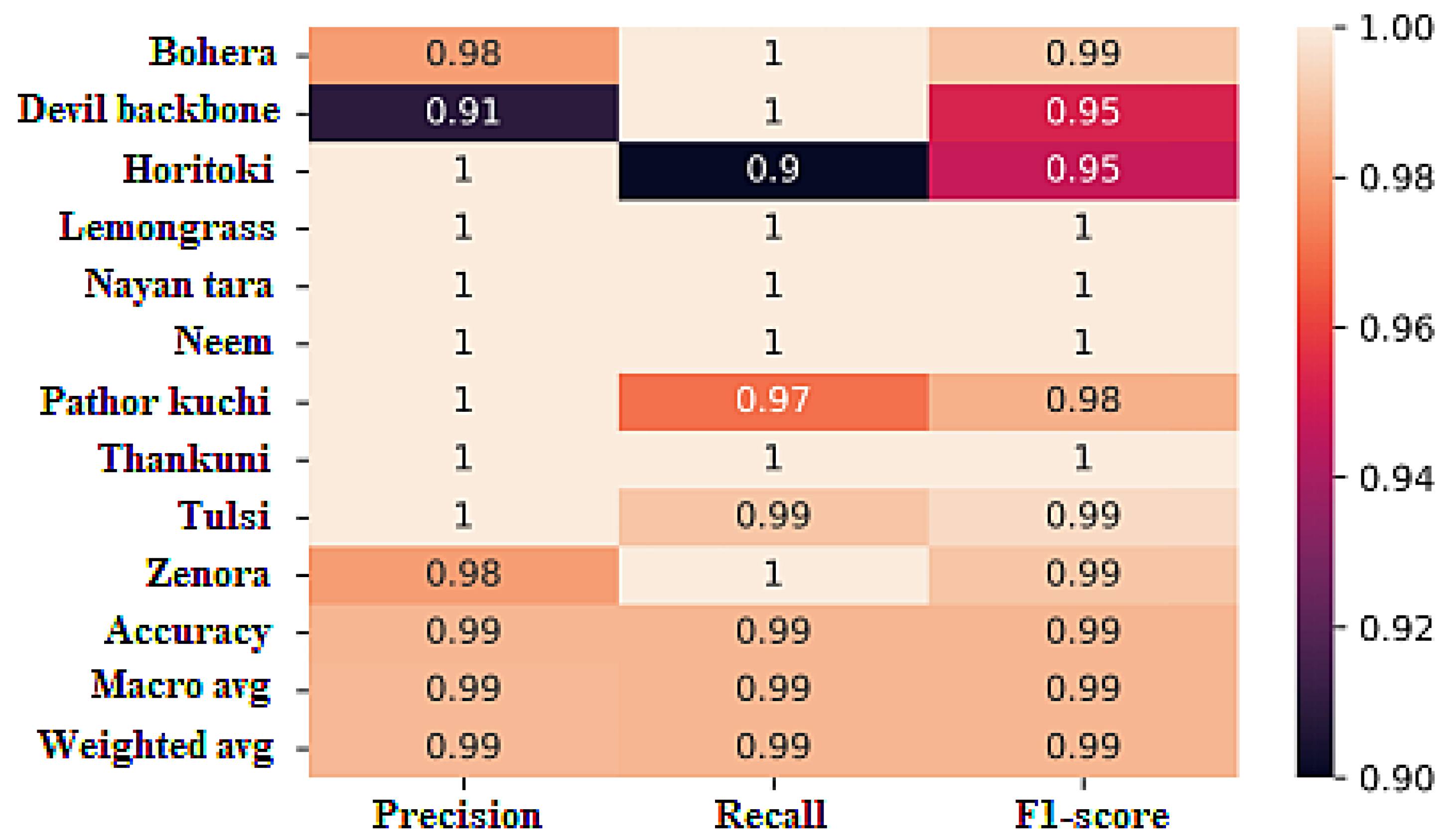
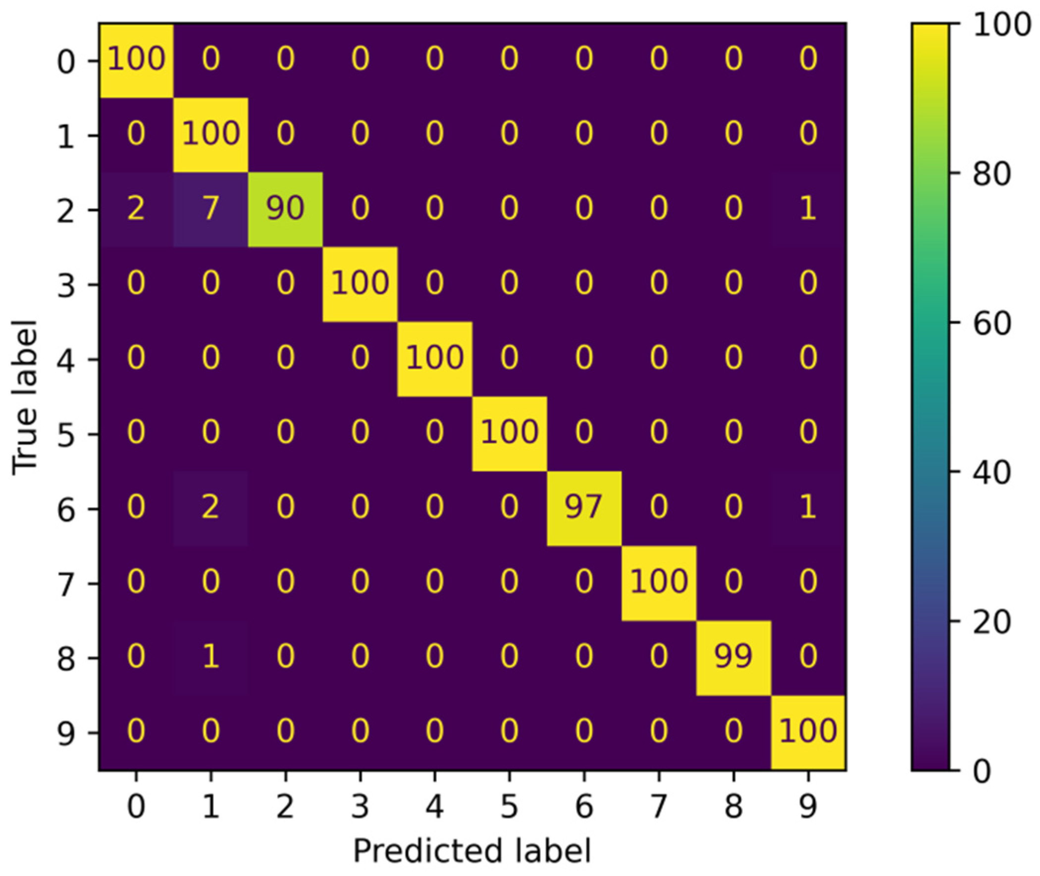
6.8. Result for the Proposed Model Using Soft Ensemble

The soft ensemble (see Figure 19), which combines the predictions of multiple models by averaging their probabilities, demonstrated outstanding results on the dataset. It achieved a remarkable accuracy of 99%, indicating that the ensemble accurately classified 99% of the instances in the dataset. The classification report and confusion matrix statistics in Figure 20 and Figure 21 provide a comprehensive evaluation of the soft ensemble’s performance.

For each class, the soft ensemble achieved excellent precision, recall, and F1 scores. Specifically, it achieved a precision of 98%, a recall of 100%, and an F1 score of 99% for the bohera class, demonstrating its ability to accurately identify instances of bohera.

For devil backbone, the soft ensemble achieved a precision of 91%, a recall of 100%, and an F1 score of 95%. Similarly, for horitoki, it achieved a precision of 100%, a recall of 90%, and an F1 score of 95%. These results highlight the ensemble’s effectiveness in accurately classifying instances of these classes.

The soft ensemble achieved perfect precision, recall, and F1 scores (100%) for the classes lemongrass, nayon tara, neem, thankuni, and tulsi, indicating flawless classification performance for these classes.

Overall, the soft ensemble exhibited exceptional performance across all evaluation metrics, with accuracy, precision, recall, and F1 scores of 99%. This highlights the ensemble’s ability to accurately classify medicinal plant species.

The confusion matrix in Figure 21 provides additional insights into the ensemble’s performance. It demonstrates the number of instances that were correctly classified and misclassified for each class. The high values along the diagonal of the confusion matrix indicate that the majority of instances were correctly classified by the ensemble.

In summary, the soft ensemble of the proposed architectures achieved outstanding performance with a high accuracy of 99% and impressive precision, recall, and F1 scores for each class. These results demonstrate the effectiveness of ensemble learning in significantly improving the overall performance of the models.

7. Discussion

In this work, we conducted a comprehensive study on the classification of ten different classes of Bangladeshi medicinal plant species. The dataset was carefully prepared, with images divided into training, testing, and validation sets. Prior to model training, we performed preprocessing steps to enhance the characteristics of the images. This included the removal of backgrounds using Adobe Photoshop’s “Remove BG” feature, followed by image processing techniques such as unsharp masking, CLAHE, and morphological gradient (3 × 3). These steps aimed to improve the quality and enhance the features of the images, providing a solid foundation for subsequent model training.

To evaluate the performance of our proposed models, we first conducted a benchmarking phase using five popular deep CNN models: VGG16, ResNet50, DenseNet201, InceptionV3, and Xception. The results obtained from Table 2 revealed that DenseNet201 achieved the highest accuracy of 85% among these benchmark models. This provided us with a reference point to gauge the performance of our developed models.

In the next stage, we introduced and applied three novel neural network architectures: DRD, DRCD, and IRCD. These architectures were specifically designed to address the challenges of classifying Bangladeshi medicinal plant species. They incorporated various components, such as dense layers, residual connections, ConvLSTM layers, and Inception modules, to capture intricate patterns and dependencies in the data. Through rigorous experimentation and training, we achieved promising results, with the DRCD model achieving the highest accuracy of 97% among the developed models. This demonstrated the effectiveness of our proposed architecture in accurately classifying medicinal plant species.

To further improve the classification performance, we employed ensemble learning techniques. Specifically, we applied both hard and soft ensembles of our developed models. The hard ensemble achieved an accuracy of 98%, while the soft ensemble outperformed all other approaches, reaching an impressive accuracy of 99%. The soft ensemble leveraged the collective intelligence of multiple models, combining their predictions to make more accurate and robust classifications. This highlights the power of ensemble learning to enhance the overall performance of the system.

Table 3. Model performance comparison of the five state-of-the-art methods with the proposed DRD, DRCD, and IRCD models and the models using hard and soft ensembles.

Model	No. of Epochs	Accuracy (%)	Precision	Recall	F1 Score
VGG16	7	67	0.67	0.67	0.65
ResNet50	8	33	0.45	0.33	0.32
DenseNet201	17	85	0.88	0.85	0.84
InceptionV3	16	76	0.81	0.76	0.74
Xception	9	67	0.76	0.67	0.64
The proposed DRD model	10	95	0.95	0.95	0.95
The proposed DRCD model	10	97	0.97	0.97	0.97
The proposed IRCD model	10	96	0.96	0.96	0.96
The proposed model using hard ensemble	-	98	0.98	0.98	0.98
The proposed model using soft ensemble	-	99	0.99	0.99	0.99

shows the comparison of the performance of the five state-of-the-art methods with the proposed DRD, DRCD, and IRCD models and the models using hard and soft ensembles.

Overall, our developed system showcased exceptional accuracy in classifying Bangladeshi medicinal plant species, achieving a remarkable accuracy of 99% through the soft ensemble. These results demonstrate the efficacy of our proposed models, the effectiveness of the preprocessing techniques applied, and the benefits of ensemble learning. The successful classification of these plant species holds great potential for applications in various domains, including medicinal research, agriculture, and biodiversity conservation.

8. Conclusions and Future Work

In this paper, we present a novel approach for medicinal plant identification using ensemble-supervised deep learning models. Our goal was to accurately classify different species of Bangladeshi medicinal plants, and we achieved an impressive identification accuracy of 99%. The results of our developed system demonstrate the effectiveness and potential of our algorithm for medicinal plant identification applications.

Through the implementation of deep learning models and ensemble learning techniques, we successfully addressed the challenges associated with classifying medicinal plant species. The proposed models, including DRD, DRCD, and IRCD, showcased high accuracy in capturing intricate patterns and dependencies within the data. Additionally, the ensemble approach further improved the overall performance, resulting in a significant boost in accuracy.

The outcomes of this research hold significant implications for various fields, including medicinal research, biodiversity conservation, and agricultural practices. Accurate identification of medicinal plant species is crucial for harnessing their therapeutic potential, understanding their ecological significance, and promoting sustainable utilization. Our developed system provides a valuable tool for researchers, botanists, and practitioners working in these domains.

Moving forward, there are several avenues for future work and improvement. Firstly, our research focused on 10 types of medicinal plant classification, but there are numerous other species with potential medicinal properties. Expanding the dataset to include a larger number of medicinal plant species would enhance the system’s capability and accuracy. This expansion can help create a comprehensive and robust medicinal plant identification system applicable to a wider range of species.

Furthermore, incorporating invariance into rotation, translation, and scaling can be explored to improve feature extraction. By incorporating these techniques, the models can become more robust and adaptable to variations in image orientations and sizes. This would further enhance the system’s performance in handling real-world scenarios where images may have different orientations and scales.

In addition, the development of user-friendly interfaces and mobile applications can facilitate the deployment of the proposed system in real-world scenarios. This would enable field researchers, herbalists, and even the general public to easily access and utilize the system for medicinal plant identification.

Overall, the successful implementation of our proposed ensemble-supervised deep learning models and the high accuracy achieved for medicinal plant identification pave the way for future advancements in this field. Further research and improvements in dataset expansion, feature extraction, and user-friendly interfaces will continue to contribute to the growth and effectiveness of medicinal plant identification systems.

In the future, we plan to expand the dataset by collaborating with experts in botany and herbal medicine to include a broader range of medicinal plant species found in Bangladesh, addressing the limitation of the dataset’s size. We will explore automated background removal techniques using image segmentation algorithms to streamline data preprocessing and enhance the model’s practicality for real-world applications. Additionally, we will investigate the integration of larger and more generalized datasets like iNaturalist, PlantCLEF, and PlantNET to improve the classification system’s robustness and generalizability, as suggested by the reviewer. These steps will strengthen the accuracy and applicability of our research.