1. Introduction
Unsupervised learning comprises all machine learning methods that are used to identify relationships among data observations with no identified dependent variable. The goal is to identify relationships among observations based on independent features of the data [
1]. Clustering methods are popular unsupervised learning methods that help identify homogeneous groupings of data observations. For data in the Euclidean space, several popular tools exist to identify clusters of similar data, such as principal component analysis (PCA) [
2], K-means clustering [
3], hierarchical clustering [
4], and density-based spatial clustering of applications with noise (DBSCAN) [
5], among others.
While supervised learning methods over tropical linear spaces are burgeoning (See [
6,
7,
8]), unsupervised learning methods for use in a tropical linear space are limited. In [
9], the authors proposed tropical principal component analysis (PCA) to estimate the best-fit polytope to data described as tropically convex. Beyond tropical PCA, unsupervised learning methods are mostly neglected and tropical analogs of Euclidean clustering methods are non-existent.
To begin to remedy the paucity of tropical unsupervised learning methods, we introduce two tropical clustering methods:
tropical K-means clustering and
tropical hierarchical clustering. Throughout this paper, we follow the methodologies shown in [
1], adapting their algorithms for use over tropically convex data. In
Section 2, this paper presents a brief overview of the tropical projective torus
with definitions and operations that are needed for our clustering techniques. In
Section 3, we introduce the tropical clustering methods, associated dissimilarity measures, and clustering analysis tools.
Section 4 provides results from computational experiments using both clustering methods. Lastly, in
Section 5, we apply tropical hierarchical clustering to the ultrametric space to illustrate its application to phylogeny.
2. Tropical Basics
In this paper, we consider the tropical projective torus
, where
is the vector with all ones in
. This means that if
, then
which means that
is isomorphic to
.
Example 1. Consider the point where . By Equation (1), . This section provides a brief overview of some necessary definitions related to tropical algebra and geometry as they pertain to the tropical clustering methods introduced in later sections. For an in-depth treatment of tropical algebra and tropical geometry, see [
10,
11].
Definition 1 (Tropical Arithmetic Operations)
. Under the tropical semiring , we have the tropical arithmetic operations of addition and multiplication, defined as follows:Note that is the identity element under addition ⊕ and 0 is the identity element under multiplication ⊙ over this semiring. Definition 2 (Tropical Scalar Multiplication and Vector Addition)
. For any and for any , we have tropical scalar multiplication and tropical vector addition, defined as follows: Definition 3. Suppose we have . If for any and for any , then S is called tropically convex.
Suppose . The smallest tropically convex subset containing V is called the tropical convex hull
or tropical polytope
of V, which can be written as the set of all tropical linear combinations of elements in VA tropical line segment
between two points , is a tropical polytope, , of a set of two points and is calculated byAs in Euclidean geometry, a tropical line segment is geodesic. Example 2. Consider the set of points . By Equation (1), . The tropical polytope defined by these points has a planar representation shown in Figure 1. The black lines between points in Figure 1 represent tropical line segments between each pair of vertices. Definition 4. For any points , the tropical distance (also known as the tropical metric) between v and w is defined as follows: Next, we remind the reader of the definition of a projection in terms of the tropical metric onto a tropical polytope. The tropical projection formula can be found in Formula 5.2.3 in [
11].
Definition 5. Let and let be a tropical polytope with its vertex set V. For , letwhere for . Thenfor all . In other words, is the projection of in terms of the tropical metric onto the tropical polytope . We are interested in the region of ambient points in terms of
. According to the projection rule, i.e., Equation (
3), two general nearby points are projected to the same position if they have the same
for all
l. This condition takes place when the minimum of
in Equation (
3) is attained at the same (say,
j-th) coordinates for all
l. Thus, we consider the region of
x, where
for all
l includes
for fixed
j, i.e.,
for all
l, so that all the points in that region have the same
. In fact,
becomes a constant, as
after
is subtracted under
. And, thus,
for all
x in the region represents the same point. This argument can be summarized as Lemma 1.
Lemma 1. Let be a tropical polytope with its vertex set , where for . Let , such that for fixed j and for all k. Then with . That is, all the points x satisfying the above inequalities are projected to the same point.
Proof. Let for all k. Then for all k and all l. Or for all k and all l. Then for all l. □
3. Tropical Clustering Methods
In this section, we introduce two tropical clustering methods. The first method we call
tropical K-means clustering, which is analogous to the Euclidean version described in [
1]. Next, we introduce
tropical hierarchical clustering. These methods are very similar to their Euclidean counterparts, with the main difference involving replacing Euclidean distance measures with the tropical metric.
3.1. K-Means Clustering in a Tropical Projective Torus
In the Euclidean space, K-means clustering is an iterative method that partitions data observations into a pre-defined set of clusters
, where cluster
and the cardinality of
based on a distance measure from the observation to the
centroid , of the cluster
[
1]. At each iteration,
for each
is calculated based on the current membership of the
. Then, data observations are reassigned based on which
is closest in terms of a distance measure. This distance measure has the effect of defining the
within-cluster variation, which becomes the measure indicating the similarity (or difference) between observations in the cluster. In [
1], the authors employ squared Euclidean distance as the method to measure within-cluster variation. This measure is defined mathematically as
where
is the
ith observation in the input data
, and
represents the number of observations assigned to cluster
. In order to assign observations to clusters, such that within-cluster variation is minimized, we arrive at the following minimization problem:
which defines K-means clustering in terms of squared Euclidean distance [
1]. Algorithm 1 shows the basic steps to conduct K-means clustering in the Euclidean space based on the squared Euclidean distance.
| Algorithm 1 K-Means clustering in the Euclidean space (from [1]) |
Input: A matrix representing data, X, where each row is an observation and the columns are the p features; set of possible clusters , and . Output: Clusters. Randomly assign each to one of the K clusters. while at least one changes the cluster assignments. do Calculate the centroid for each cluster . Assign each to the cluster, , where the Euclidean distance from to is minimized. end while return .
|
Tropical K-means clustering is analogous to K-means clustering in the Euclidean space with the exception of using the tropical metric in lieu of the Euclidean distance as a measure of within-cluster variation. To begin, we first introduce Algorithm 2, which shows the basic steps of executing K-means clustering in the tropical projective torus. Note that Algorithm 2 mimics Algorithm 1, except that instead of a centroid defined by a point where each coordinate represents an in-cluster feature average, we now define the centroid in terms of the
Fermat–Weber point using the tropical distance.
| Algorithm 2 K-means clustering in the tropical projective torus. |
Input: A matrix representing data, X, where each row is an observation and the columns are the e features; the desired number of clusters: K. Output: Clusters. Randomly assign each to one of the K clusters. while at least one changes the cluster assignment. do Calculate the F-W point , for each cluster . Assign each to the cluster, , where is minimized. end while return .
|
Calculating a Tropical Fermat–Weber Point
As mentioned in [
12], because of the non-Euclidean nature of tropical geometry, it is natural to use the
Fermat–Weber points of a given sample defined in Equation (
6). In tropical K-means clustering, we use the tropical Fermat–Weber point to represent the centroid of each cluster. In general, for a given set of observations,
X, where
, the Fermat–Weber point is a point,
y, which satisfies
where
represents a distance measure and
. A tropical Fermat–Weber point is similarly defined, except using the tropical metric. Therefore, the tropical Fermat–Weber point
satisfies
The Fermat–Weber point
u, calculated from (
6), provides the representation of a centroid based on the tropical metric. For each iteration of Algorithm 2, we recompute a Fermat–Weber point for each cluster as long as observations continue to be reassigned to different clusters. A possible challenge to using the tropical Fermat–Weber point is that the point may not be unique. Therefore, it is conceivable that the cluster membership may not change when it should, or the converse. This bears further research and exploration. For a thorough discussion on tropical Fermat–Weber points, see [
13].
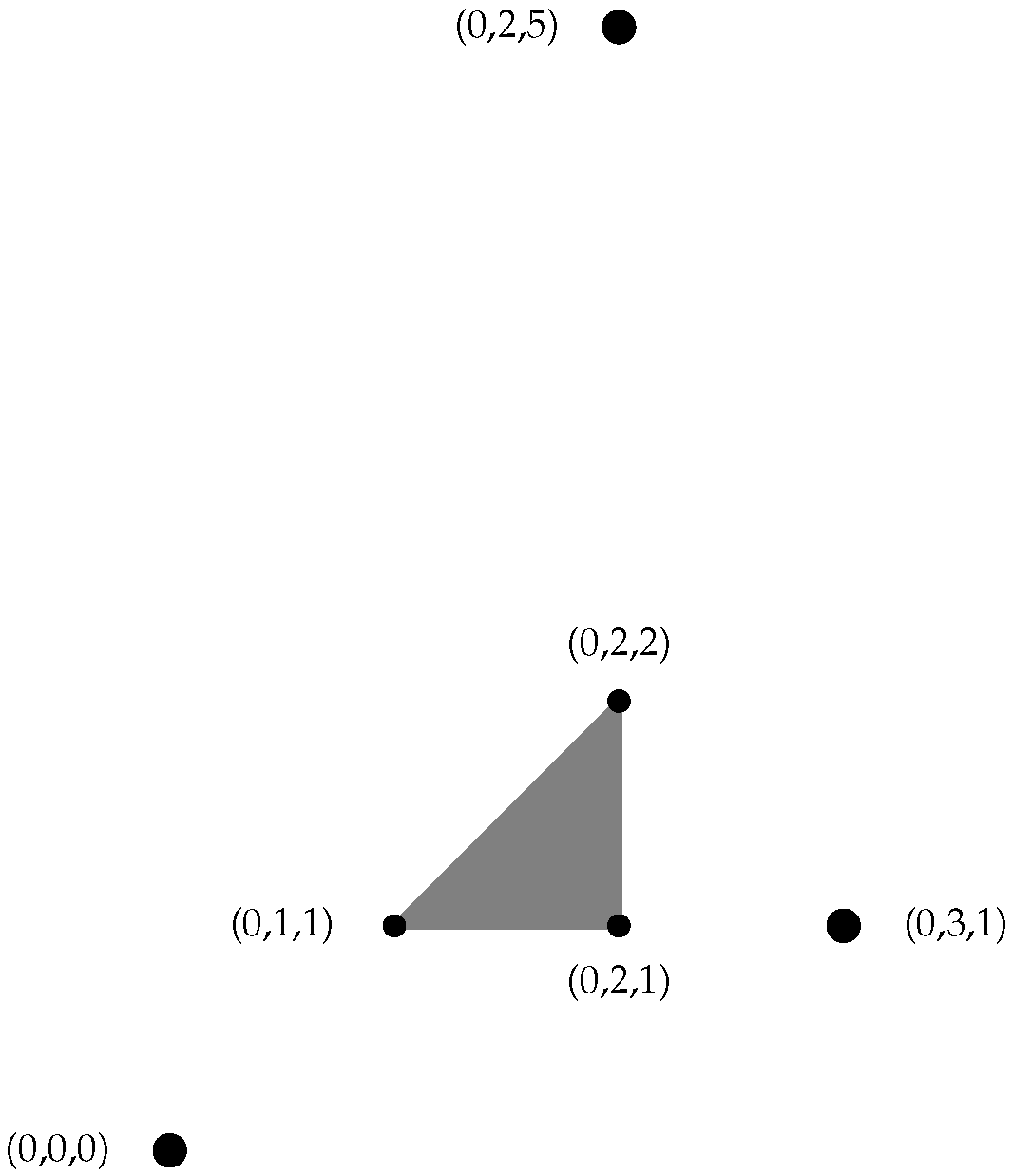
Example 3. Consider the points (recall Equation (1)) in that are members of cluster . Let the point have membership in cluster . The gray triangle in Figure 2 shows the Fermat–Weber region for the points in , meaning that any point contained in the triangle represents a tropical Fermat–Weber point satisfying (6). Letting the vertices of the triangle be represented by , , and , we calculate , , and . If we let represent the Fermat–Weber point for , and , it is possible that y retains membership to , even though there are points in the Fermat–Weber region of that are closer, according to the tropical metric. Using the F-W point to represent the centroid of a cluster, we now introduce Algorithm 2 to define K-means clustering over the tropical projective torus.
As can be seen in Algorithm 2, there are two main steps after initialization. First, we calculate
for each
defined by the current membership of
. The second step involves calculating
for each
and assigning
to
, such that
is minimized. The goal for K-means clustering over
is to minimize a cost function that is similar to (
4), but instead of using the squared Euclidean distance as a measure of the within-cluster variation, we replace it with the tropical metric. This leaves us with the following objective function, minimizing within cluster variation
where
with
is the number of elements in the cluster
.
3.2. Hierarchical Clustering over the Tropical Projective Torus
Another method of clustering often used in the Euclidean space is hierarchical clustering. Unlike K-means clustering, hierarchical clustering does not require a predetermined number of clusters to assign observations. Instead, hierarchical clustering combines observations into clusters by progressively calculating what we call the
inter-cluster distance using a dissimilarity measure [
1]. In the Euclidean space, there are several dissimilarity measures available. For a list of the more popular dissimilarity measures, see Table 10.2 in [
1]. Algorithm 3 shows a generic hierarchical clustering algorithm in the Euclidean space.
| Algorithm 3 Hierarchical Clustering in the Euclidean Space (from [1]) |
Input: A matrix X representing data with rows being the observations, with each row being a point , the columns are the e features, and represents the number of observations; dissimilarity measure. Output: Set of clusters for each iteration. Let each represent a cluster. for i = |X|,…,2 do Examine all pairwise inter-cluster distances. Fuse the two clusters with the smallest inter-cluster distance. Compute pairwise inter-cluster distances of the remaining clusters. end for return .
|
Algorithm 3 begins by allowing each observation to represent its own cluster. Then using the dissimilarity measure, clusters are grouped pairwise at each step until all observations are grouped together in a single cluster. Additionally, at each iteration, the value of the dissimilarity measure is captured. One (informal) way to determine the number of clusters in the data is to examine the dissimilarity measure between two iterations. If the dissimilarity measure from the current iteration to the next is very large, then this can provide an indication of separation between clusters in the current iteration.
Visually, this progressive fusing of clusters has a tree representation known as a
dendrogram. The dendrogram resulting from hierarchical clustering consists of
and
axes, where the
axis shows the observations. The
axis represents the dissimilarity measure (often called the height) between clusters as they fuse.
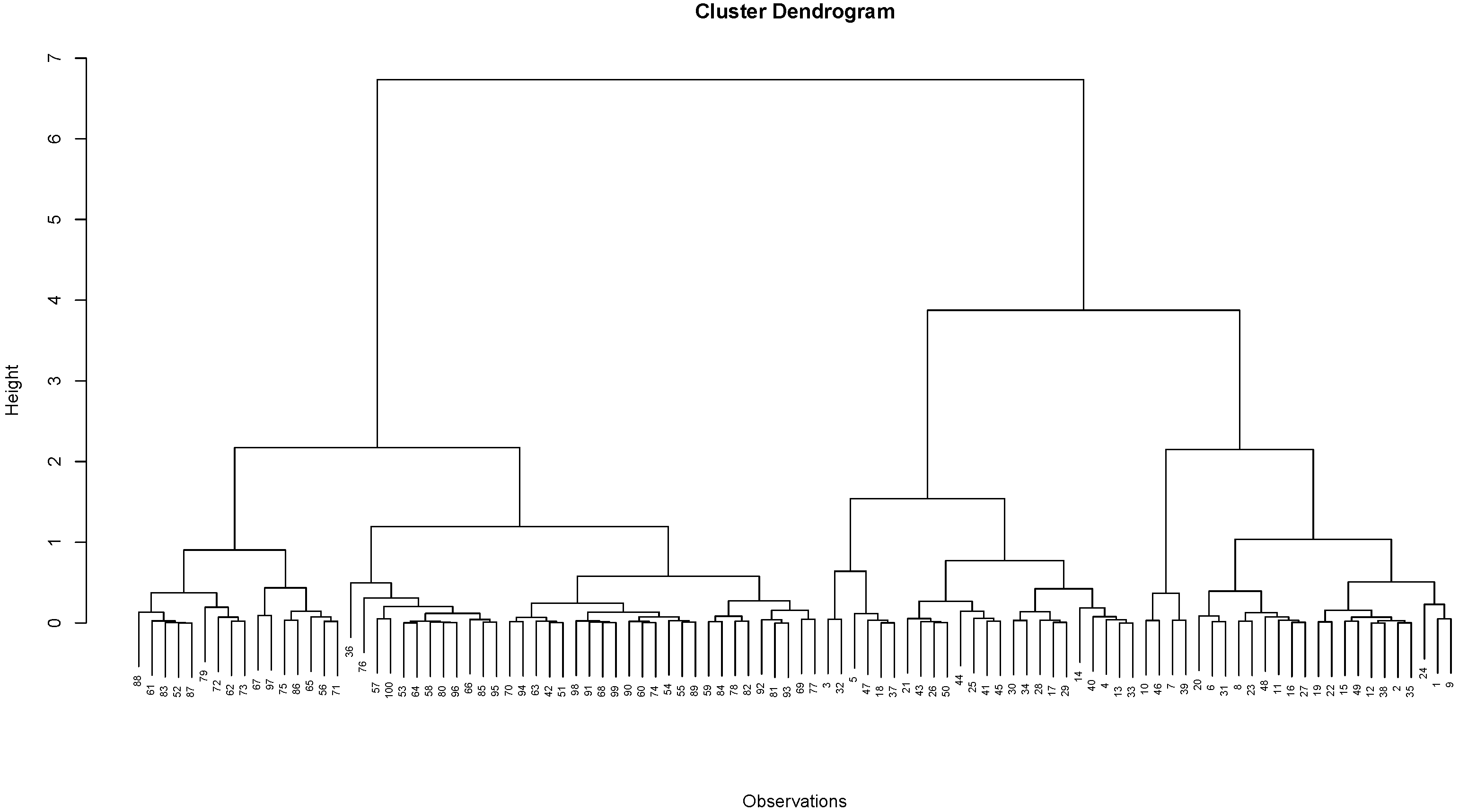
Figure 3 provides an example of a dendrogram after hierarchical clustering was employed on
observations of simulated data, where 50 points each were taken from two Gaussian distributions with differing mean and standard deviation parameters.
3.3. Dissimilarity Measures for Tropical Hierarchical Clustering Using Pairwise Distances
The most popular dissimilarity measures used in classical hierarchical clustering employ the Euclidean distance [
1]. We can use a similar approach for tropical hierarchical clustering by replacing the Euclidean distance with the tropical distance. Tropical dissimilarity measures (or
tropical linkages) using pairwise tropical distances are defined in a similar fashion as linkages in the Euclidean space.
Table 1 shows summaries of tropical pairwise dissimilarity measures.
Definition 6 (Tropical Pairwise Complete Linkage)
. The tropical complete linkage
between two clusters, and , is a dissimilarity measure determined by identifying points and , where is the largest. This is defined mathematically as Example 4. Consider clusters , and (0,6,4), . Figure 4 and Figure 5 illustrate which points in define the dissimilarity for each dissimilarity measure we consider for tropical hierarchical clustering. Definition 7 (Tropical Pairwise Single Linkage)
. For two clusters, and , a tropical single linkage
is determined by and , where is minimized. That is
Figure 5.
Tropical pairwise single linkage for Example 4. The single linkage defined by the red tropical line segment as calculated by Equation (
2), representing the minimum distance between a pair of vertices defining the polytope in each cluster.
Figure 5.
Tropical pairwise single linkage for Example 4. The single linkage defined by the red tropical line segment as calculated by Equation (
2), representing the minimum distance between a pair of vertices defining the polytope in each cluster.
Definition 8 (Tropical Pairwise Average Linkage)
. For a given cluster , the tropical pairwise average linkage
between and a separate cluster is given by taking the average of over all . Specifically, A benefit to defining tropical linkages as shown in
Table 1 is that we can leverage the functionality of the
hclust function in
R because its input is an
R distance object. This allows us to build dendrograms as we would using Euclidean distances.
Dissimilarity Measures for Tropical Hierarchical Clustering Using Projections
An alternative to pairwise tropical distances between points in different clusters is to calculate the tropical distance between a point in a cluster and its projection onto another cluster. A cluster of points in the tropical projective torus is a tropically convex set that can be defined as a tropical polytope. We denote the tropical polytope defined by the points in cluster as . To determine the dissimilarity between two clusters, and , we can project each point from onto . The projection of a point onto is the point in that is closest in terms of the tropical distance to the point being projected. Calculating the distance between a point and its projection provides the basis of a dissimilarity measure.
For a cluster of points in
, we say the dissimilarity measure, or
linkage, relative to another cluster is determined by the tropical distance between each point and its projection onto the tropical polytope defined by another cluster [
1]. Here, we let
represent the
ith point in cluster
, and
represent the projection of
onto the cluster
, as defined by (
3). The definitions that follow describe the linkages we consider in this paper, which we call
tropical complete linkage,
tropical single linkage, and
tropical average linkage.
Table 2 summarizes these linkages.
Definition 9 (Tropical Complete Linkage)
. The tropical complete linkage
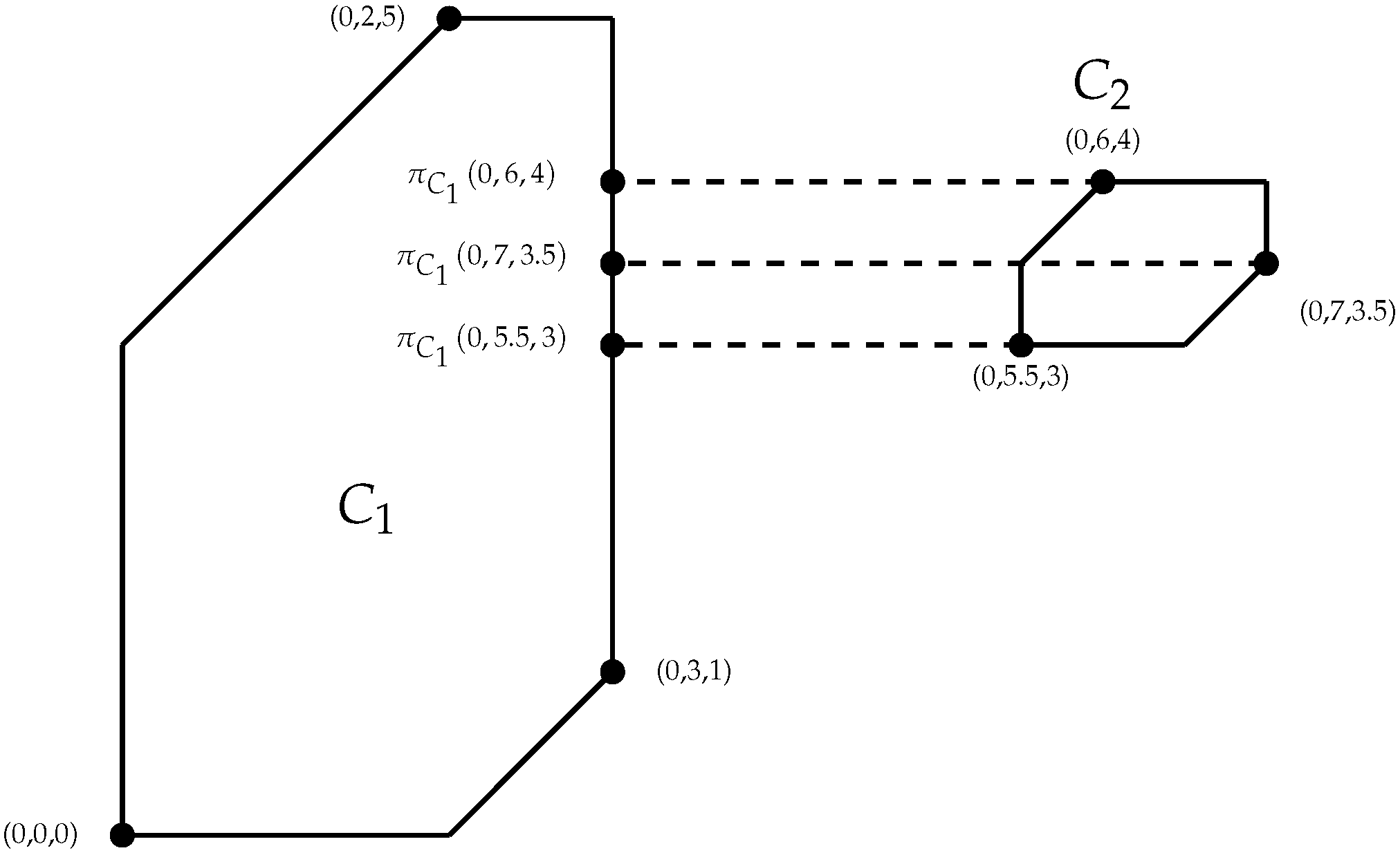
between two clusters, and , is a dissimilarity measure determined by identifying point , where is the largest. This is defined mathematically as Example 5. Consider clusters and , . Figure 6, Figure 7 and Figure 8 illustrate which points in define the dissimilarity for each of the dissimilarity measures we consider for tropical hierarchical clustering. Definition 10 (Tropical Single Linkage)
. For two clusters, and , a tropical single linkage is determined by the , such that is minimized. That is
Figure 7.
Tropical single linkage for Example 4. The dotted line represents the projection of
onto
as calculated using Equation (
3).
Figure 7.
Tropical single linkage for Example 4. The dotted line represents the projection of
onto
as calculated using Equation (
3).
Definition 11 (Tropical Average Linkage)
. For a given cluster , the tropical average linkage between and a separate cluster is given by taking the average of over all . Specifically,
Figure 8.
Tropical average linkage for Example 4. The dotted lines represent the projections of each vertex in
onto
as calculated using Equation (
3). Note that we average the tropical distances to determine the linkage between
and
.
Figure 8.
Tropical average linkage for Example 4. The dotted lines represent the projections of each vertex in
onto
as calculated using Equation (
3). Note that we average the tropical distances to determine the linkage between
and
.
Algorithm 4 provides the general algorithm associated with tropical hierarchical clustering.
| Algorithm 4 Hierarchical clustering in the tropical projective space |
Input: A matrix X representing data with rows as the N observations, where each is a point , the columns are the e features, and represents the number of observations; tropical dissimilarity measure. Output: Set of clusters for each iteration. Let each represent a cluster. for i = n,…,2 do Examine all pairwise inter-cluster dissimilarities. Fuse the two clusters with the smallest inter-cluster dissimilarity. Compute the pairwise inter-cluster dissimilarity of remaining clusters. end for return .
|
3.4. Cluster Analysis
In the experiments that follow in the next section, we will apply the tropical clustering algorithms to simulated data that can be analyzed visually. However, in most cases, the dimensions of the data are too large for us to visualize, so we must establish some metrics to analyze the cluster results. Leveraging terminology from graph theory, in this section, we provide metrics that we call tropical withiness and tropical betweenness.
Definition 12 (Average Tropical Withiness)
. Consider a cluster, , generated from a tropical clustering algorithm. Average tropical withiness, denoted as , is an indication of the relationship of the data in . Mathematically, we define it as Definition 13 (Maximum Tropical Withiness)
. Consider a cluster, , generated from a tropical clustering algorithm. Maximum tropical withiness, denoted as , is an indication of outliers in a cluster. Mathematically, we define it as Definition 14 (Tropical Betweenness)
. Consider two clusters, and , generated from a tropical clustering algorithm. Tropical betweenness, denoted as , is an indication of the relationship between clusters and . Formally, tropical betweenness is defined as Because tropical betweenness is measured in terms of the tropical distance from a point in a cluster to its projection onto the tropical polytope defined by another cluster, the betweenness measured from cluster
to cluster
will likely be different than the betweenness measured from
to
. However, the values should be relatively close, so we use the average of the two measures. That is,
Neither tropical withiness nor betweenness alone provides sufficient information describing the clusters or their relationships with each other. However, relating the two can provide some information on the overall relationship between points in the cluster and the clusters themselves. One such method is to take the ratio of withiness to betweenness, denoted as
and defined as
A large value of suggests that is not very dense and the tropical distance between and is small. Such a situation could indicate some overlap between sub-groups of data points and difficulty identifying meaningful clusters. A small value of may indicate that data points assigned to are close in terms of tropical distance relative to the distance of the cluster to . In this situation, clusters may be separated with little overlap in the data. In the section that follows, we will see examples of well-separated data and overlapping data as well as the challenges that overlapping data pose to our tropical clustering methods.
4. Computational Experiments
In this section, we conduct computational experiments using tropical k-means and hierarchical clustering methods. In each case, we generate random points in
using a Markov Chain Monte Carlo (MCMC) hit-and-run (HAR) method that samples tropical points from a tropical polytope by employing a Gaussian kernel. The sampler takes the user-defined location and scale parameters,
and
, respectively, [
15]. The sampler mimics a Gaussian HAR sampler in the Euclidean space with
controlling the dispersion of points sampled at about
, which serves as a centroid. In addition, we apply tropical K-means clustering to the iris data set from the
MVTests package version 2.1.1 in
R.
For each of our clustering methods, we conduct two experiments on sampled points divided into three groups of 50 points. Each group is sampled using different locations and scale parameters. In this first experiment, 50 points are sampled with and , 50 points are sampled using and ; moreover, 50 points are sampled using and . The obtained sample represents a situation where there is separation between each of the groups that make up the sample.
The second experiment samples points as well. In this case, 50 points are sampled using parameters and ; 50 points are sampled using and ; and 50 points are sampled using and . There is significant overlap between the points, making it more difficult to distinguish between groups.
4.1. Tropical K-Means Clustering
We begin by applying tropical K-means clustering to each of the two samples described above.
4.1.1. Experiment 1
In this first experiment, we observe the simulated data in
Figure 9. The data are colored according to the parameter sets from which they emanated.
Applying Algorithm 2 to the input of the
-pre-defined clusters, we observed that the three original groups are defined and membership is almost perfectly assigned according to the true assignment.
Figure 10 shows the progression of Algorithm 2.
For this experiment, the algorithm took five iterations to finalize the cluster assignment. Only five observations are incorrectly assigned. For the three clusters, we also calculate
. The final assignment of clusters is shown in the bottom right plot in
Figure 10.
is the cluster of black points with
;
is the cluster of red points with
; and
is the cluster of green points with
.
4.1.2. Experiment 2
This experiment highlights the challenge of identifying clusters where observations overlap.
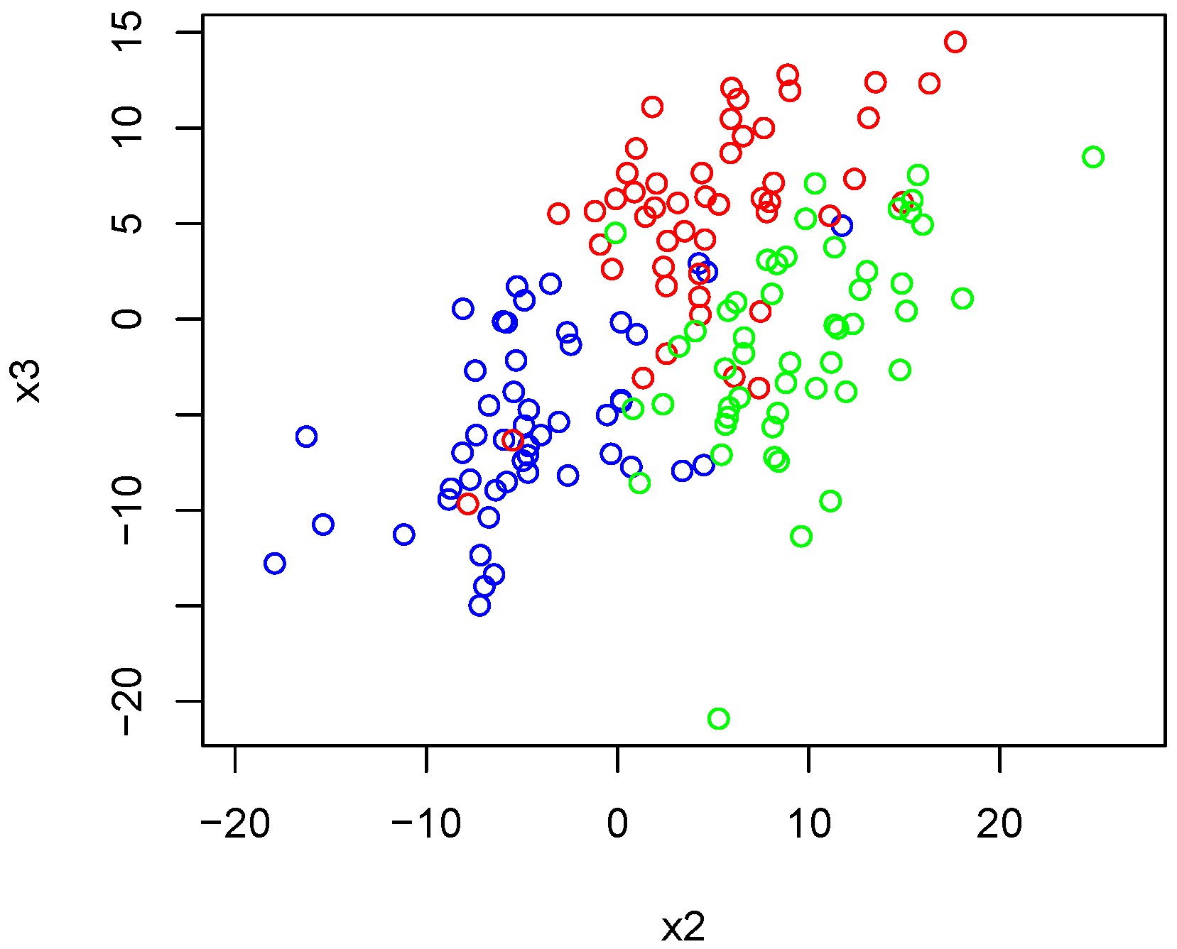
Figure 11 shows the observations as sampled using the Gaussian-like MCMC HAR sampler. There is a noticeable (intentional) overlap in the observations.
The results from this experiment are shown in
Figure 12, which shows the progression of cluster assignments for the observations. The top left pane shows the starting assignment with the top right and bottom left plots showing the first and second iterations, respectively. The final assignment is shown in the bottom right plot. It took six iterations to finalize the cluster assignment.
Algorithm 2 identifies the three clusters in their relative positions to each other; it has a higher incorrect assignment rate. In total, 19 of the 150 observations were assigned to the incorrect cluster. This is somewhat expected since there is significant overlap amongst the observations. For the three clusters, we calculate
. Referencing the bottom right plot in
Figure 12,
is the set of green points with
;
is the group of red points with
; the last group of black points,
, has
. These values are noticeably, though not surprisingly, higher than the results in experiment 1. The clusters lie adjacent to each other, resulting in a small betweenness value. Also, the points in each cluster are not tightly concentrated around their respective calculated centroids.
4.1.3. Iris Dataset
In this section, we apply tropical K-means clustering to the iris dataset from the
MVTests package in
R. The data consist of 150 observations on four features. In these data, there is a multinomial response variable, where each observation is classified as one of three species of the iris flower. For each species, the observation numbers classified by species type are
. In this experiment, we remove the response variable and see how well our tropical K-means clustering method correctly clusters data compared to the Euclidean K-means clustering method. For both methods, we scale the data before applying the clustering method. The results are shown in
Table 3 with
representing the actual counts of each species and
representing the counts of each type in each cluster.
In both cases, we scale the data prior to applying the clustering method and we achieve similar results. Tropical k-means clustering provides slightly better results in this case, with a correct cluster assignment rate of versus a correct cluster assignment rate of .
4.2. Tropical Hierarchical Clustering
Now, we turn our attention to tropical hierarchical clustering described in Algorithm 4. We apply Algorithm 4 to similar observations as those used for tropical K-means clustering.
The goal of this experiment is to determine how well Algorithm 4 correctly determines the clusters using the different linkages. As is clear from Algorithm 4, there will be N iterations in the algorithm until all points are members of a single cluster. Since we know that there are three groupings of sampled points associated with different scales and location parameters, the goal would be to see three clusters with correct membership, no later than iteration 148.
4.2.1. Experiment 1
In this first experiment, we sample
points using the Gaussian-like tropical HAR sampler, where we sample
points using the Gaussian-like tropical HAR sampler. In this experiment, 50 points are sampled with
and
, 50 points are sampled using
and
, and 50 points are sampled using
and
. We then apply Algorithm 4 using each of the dissimilarity measures defined in the previous section.
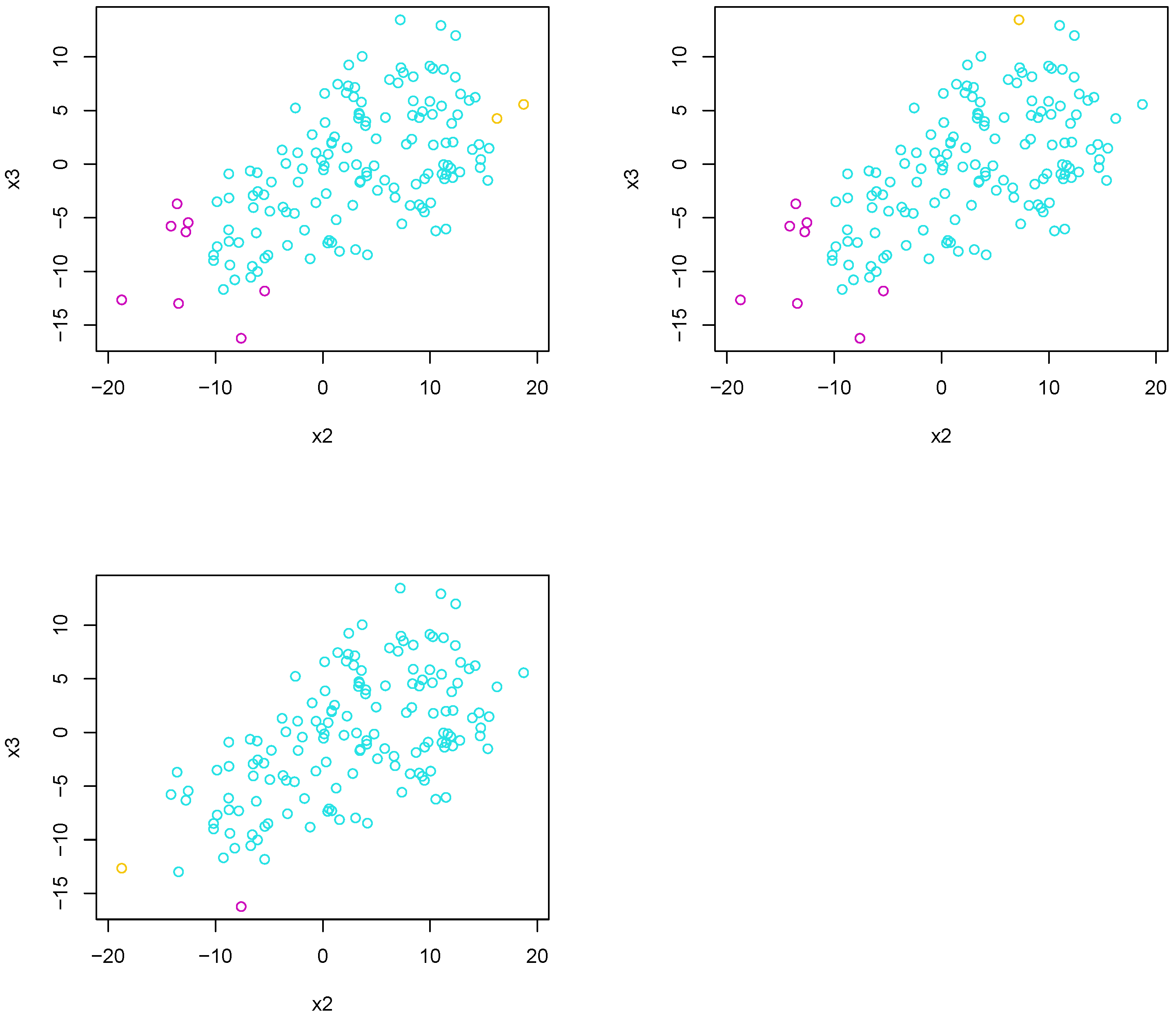
Figure 13 shows the sampled points differentiated by color. We see that the groups of the sampled are visually separable. We then apply Algorithm 4 using each of the dissimilarity measures defined in the previous sections.
Figure 13 shows the sampled points differentiated by color. We see that the groups of samples are visually separable.
Figure 14 shows the results using tropical average (top left), tropical complete (top right), and tropical single (bottom) linkages.
The tropical complete linkage provided the best results, perfectly assigning all points to clusters associated with their locations and scale parameters. For each of the three clusters defined using the complete linkage, we also calculated . In this case, is the cluster of blue points, is the cluster of magenta points, and is the cluster of yellow points. For each cluster, we have , , and .
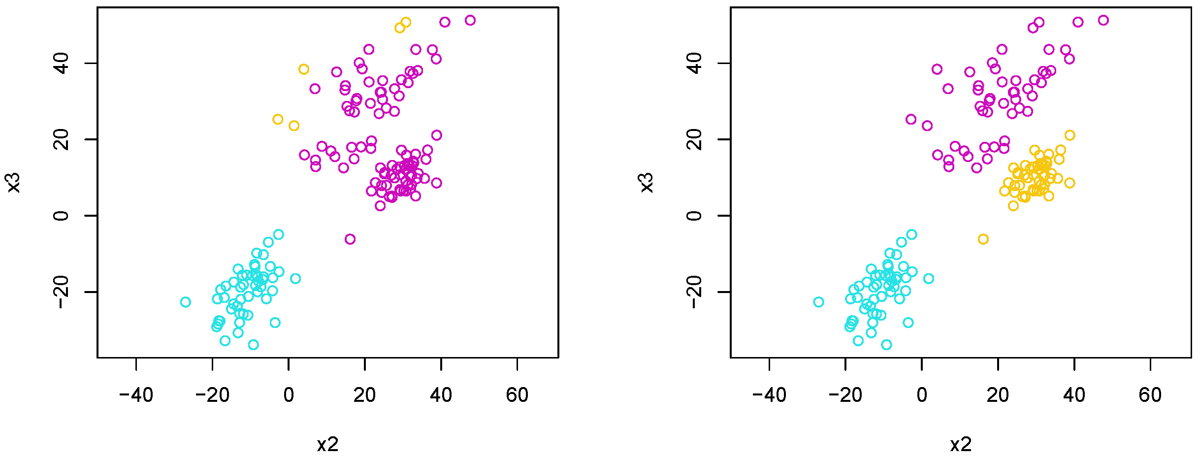
4.2.2. Experiment 2
Now, we want to observe how well Algorithm 4 identifies clusters, where there is overlap amongst sampled points.
Figure 15 shows the sampled points differentiated by color.
Because the groupings overlap, it is difficult for the algorithm to discern between different clusters. Regardless of which dissimilarity measure is used, clustering results lead to one very large cluster and two small clusters, consisting of only a handful of points.
Figure 16 shows the result for each linkage.
In terms of hierarchical clustering, the complete linkage seems to outperform the others; however, for experiment 2, all linkage methods performed poorly. With that in mind, we forego calculating associated clustering metrics.
Between the two clustering methods, tropical K-means performed better in terms of identifying and correctly assigning observations to the correct cluster. However, as we will see in the following sections, K-means clustering is not always a viable option for the given data.
5. Applications to Phylogenetic Trees
A phylogenetic tree is a tree representation of evolutionary history among given species. In this paper, we focus on
equidistant tree, which is a rooted phylogenetic tree whose distance from its root to each leaf is the same for all leaves. Equidistant trees can be viewed as inferred phylogenetic trees in terms of the molecular clock. When inferring the species tree, which is a phylogenetic tree of a given set of species, from gene trees (the phylogenetic trees inferred from each gene) under the multi-species coalescent model, we assume that all phylogenetic trees in the input sample are equidistant trees [
16].
Phylogenomics is a new field that applies tools from phylogenetics to genome data. In phylogenomics, we conduct statistical analyses on a sample of gene trees over the space of phylogenetic trees, which is a set of all possible phylogenetic trees with a given set of labels of leaves, i.e., species. However, the space of phylogenetic trees is not Euclidean and it is a union of lower dimensional polyhedral cones with co-dimension
over
, where
m is the number of leaves [
17,
18,
19]. Therefore, if we apply classical statistical methods to a sample of phylogenetic trees, the results from such methods might lead to misleading conclusions.
In 2006, Ardila and Klivans showed that the space of equidistant trees is a tropical linear space. Therefore, if we apply the tropical metric, we can use tropical linear algebra to conduct statistical analyses over the space of equidistant trees. For example, Yoshida et al. applied the tropical metric to the principal component analysis over the space of equidistant trees [
9].
In this section, we apply hierarchical clustering of the space of phylogenetic trees on
m leaves. We specifically focus on hierarchical clustering because obtaining a Fermat–Weber point, as is required in tropically K-means clustering, may not be in the space of equidistant trees [
13]. In the sections that follow, we will review the definition of
ultrametrics and its relation to the space of phylogenetic trees. Then, we will use hierarchical clustering to identify varying tree topologies over the ultrametric space
.
5.1. Basics of Ultrametrics
Let
. Suppose a map
is a metric over
. This means that
u has to satisfy the following conditions:
Suppose
u is a metric on
. Then, if
u satisfies the following condition, which is a stronger condition on the triangle inequality:
then, we call
u an
ultrametric.
Example 6. Suppose . Then, a metric u on , such thatis an ultrametric. A phylogenetic tree is a weighted tree whose internal nodes do not have labels and whose external nodes, i.e., leaves, have labels. We consider a rooted phylogenetic tree with a given leaf label set .
Definition 15. Suppose we have a rooted phylogenetic tree T with a leaf label set . If the total branch length in a unique path from its root to each leaf is the same for all , then we call T an equidistant tree.
In order to conduct any statistical analysis related to phylogenetic trees, we must map a phylogenetic tree with to a vector representation. One way to map a phylogenetic tree to a vector is to map it to a dissimilarity map. This leads to the two following definitions.
Definition 16 (From [
20])
. A dissimilarity map d is a function , such that and for each pair . We can represent a dissimilarity map d by an matrix whose entry is . Because is symmetric and all diagonal entries are zeros, we can regard d as a vector, where .
Definition 17 (From [
20])
. Let T be a phylogenetic tree with m leaves labeled with the elements of . Assign a length to each edge . Define , such that is the total length of the unique path from leaf i to leaf j. We call a function d obtained in this way a tree distance. Further, if each entry of the distance matrix is non-negative, then d is a metric. We call such a tree distance a tree metric.
This allows us to embed D into , where . In phylogenetics, we consider dissimilarity maps over the product of a leaf set , where is the pairwise distance between a leaf to leaf . The vector of all possible pairwise distances in T between any two leaves in provides a representation of a phylogenetic tree T with leaf label set . This leads to the following theorem.
Theorem 1 ([
21])
. Suppose we have an equidistant tree T with a leaf label set and suppose for all is a distance from leaf i to leaf j. Then, u is an ultrametric if and only if T is an equidistant tree. Using Theorem 1, if we consider the spaces of all possible equidistant trees, then we can consider the ultrametric space over , , as the space of phylogenetic trees on .
5.2. Hierarchical Clustering over the Space of Ultrametrics
In this section, we apply tropical hierarchical clustering methods to the space of phylogenetic trees over
m leaves, represented as the ultrametric space,
. The reason we focus on tropical hierarchical clustering (as opposed to tropical K-means clustering) is simple: tropical K-means clustering defined in Algorithm 2 requires computing Fermat–Weber points, but the resulting points may not be ultrametrics, potentially leading us to false conclusions [
13]. Tropical hierarchical clustering requires no such calculation. In a case of ultrametrics, we use the DIvisie ANAlysis (DIANA) clustering algorithm [
22] with tropical distances (metrics) between all pairs of ultrametrics in a given sample.
We generate equidistant trees from the multi-species coalescent model with a given species tree using
Mesquite [
23]. Under the multi-species coalescent model, there are two parameters:
species depth (SD) and
effective population size . We fix
and we vary SD by the ratio
R, such that
For each
, we generate two independent samples. For each sample, we generate a sample of 1000 gene trees from a multi-species coalescent model with a fixed species tree. These two independent samples for a fixed
R have different species of trees. Note that it is well-known that the smaller the
R, the harder to classify two different multi-species coalescent models (for example, [
24]).
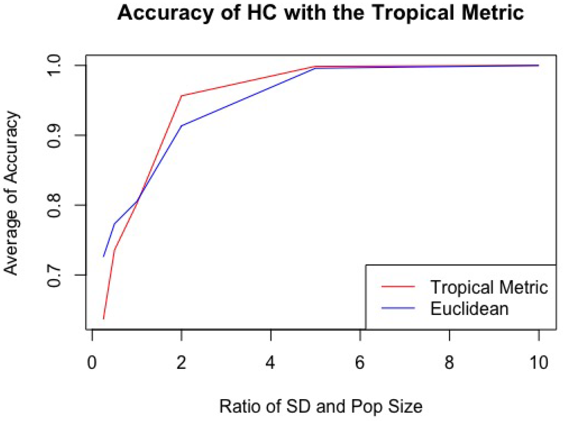
In this computational experiment, we fix
, which means
. We sample random 20 trees from each sample and we repeat 100 times to estimate the accuracy rates for clustering by different distributions. In
Figure 17, we plot the averages of accuracy rates from 100 repeats for each ratio
R. We also compare the accuracy rates against DIANA with the Euclidean metric (
norm).
6. Conclusions
In this paper, we introduced two tropical clustering tools used for tropical unsupervised machine learning. Tropical K-means clustering is the analog of the Euclidean K-means clustering method. Instead of a Euclidean distance, we incorporate the tropical metric, and centroids are calculated by finding the tropical Fermat–Weber points for each cluster instead of using feature means. Tropical hierarchical clustering mimics Euclidean hierarchical clustering by using dissimilarity measures to progressively fuse clusters together at each iteration of Algorithm 4. Instead of computing dissimilarities using pairwise distances between points in one cluster with points in another, we calculate the distance between a point in one cluster and its projection onto the tropical polytope, defined by the points in another cluster. In each case, cluster analysis metrics are introduced to understand how well-separated clusters are as well as the relationship between points in each cluster.
Computational experiments showed that both methods can be effective, as long as clusters are well-separated. Tropical K-means clustering provided promising results regardless of the overlap of data; however, because of some tropically convex data, such as data defined as ultrametrics, a Fermat–Weber point will not necessarily be ultrametric, making this technique potentially ineffectual in such a case. In tropical hierarchical clustering, the tropical complete linkage provided the best overall cluster assignment. Further, in analyzing the space of equidistant trees on m leaves, it performed well if we used DIANA on the tropical metric as the distance measure on trees for computing all pairwise distances between trees in a given sample.
Author Contributions
Methodology, D.B. and R.Y.; Software, D.B. and R.Y.; Data curation, R.Y. All authors have read and agreed to the published version of the manuscript.
Funding
This research was funded by National Science Foundation grant number DMS 1916037.
Data Availability Statement
Not applicable.
Acknowledgments
The authors thank all the reviewers for their comments and suggestions, which improved the manuscript. R.Y. and D.B. are partially supported by NSF DMS 1916037.
Conflicts of Interest
The authors declare no conflict of interest.
References
- James, G.; Witten, D.; Hastie, T.; Tibshirani, R. An Introduction to Statistical Learning: With Applications in R; Springer: Berlin/Heidelberg, Germany, 2013. [Google Scholar]
- Hotelling, H. Analysis of a Complex of Statistical Variables Into Principal Components. J. Educ. Psychol. 1933, 24, 417–441, +498–520. [Google Scholar] [CrossRef]
- MacQueen, J. Classification and analysis of multivariate observations. In Proceedings of the 5th Berkeley Symposium on Mathematical Statistics and Probability; University of California: Los Angeles, CA, USA, 1967; pp. 281–297. [Google Scholar]
- Anderberg, M.R. Cluster Analysis for Applications; Academic Press: Cambridge, MA, USA, 1973. [Google Scholar]
- Ester, M.; Kriegel, H.P.; Sander, J.; Xu, X. A Density-Based Algorithm for Discovering Clusters in Large Spatial Databases with Noise. Knowl. Discov. Data Min. 1996, 96, 226–231. [Google Scholar]
- Akian, M.; Gaubert, S.; Qi, Y.; Saadi, O. Tropical Linear Regression and Mean Payoff Games: Or, How to Measure the Distance to Equilibria. SIAM J. Discret. Math. 2023, 37, 632–674. [Google Scholar] [CrossRef]
- Yoshida, R.; Takamori, M.; Matsumoto, H.; Miura, K. Tropical Support Vector Machines: Evaluations and Extension to Function Spaces. 2021. Available online: https://arxiv.org/abs/2101.11531 (accessed on 10 June 2023).
- Yoshida, R. Tropical Balls and Its Applications to K Nearest Neighbor over the Space of Phylogenetic Trees. Mathematics 2021, 9, 779. [Google Scholar] [CrossRef]
- Yoshida, R.; Zhang, L.; Zhang, X. Tropical Principal Component Analysis and its Application to Phylogenetics. Bull. Math. Biol. 2019, 81, 568–597. [Google Scholar] [CrossRef] [PubMed]
- Joswig, M. Essentials of Tropical Combinatorics; Graduate Studies in Mathematics; American Mathematical Society: Providence, RI, USA, 2022. [Google Scholar]
- Maclagan, D.; Sturmfels, B. Introduction to Tropical Geometry; Graduate Studies in Mathematics; American Mathematical Society: Providence, RI, USA, 2015; Volume 161. [Google Scholar]
- Lin, B.; Sturmfels, B.; Tang, X.; Yoshida, R. Convexity in Tree Spaces. SIAM Discret. Math 2017, 3, 2015–2038. [Google Scholar] [CrossRef]
- Lin, B.; Yoshida, R. Tropical Fermat–Weber Points. SIAM Discrete Math. 2018, 32, 1229–1245. [Google Scholar] [CrossRef]
- R Core Team. R: A Language and Environment for Statistical Computing; R Foundation for Statistical Computing: Vienna, Austria, 2023. [Google Scholar]
- Barnhill, D. Markov Chain Monte Carlo Sampling of Tropically Convex Sets. Ph.D. Thesis, Naval Postgraduate School, Monterey, CA, USA, 2024. in press. [Google Scholar]
- Rannala, B.; Edwards, S.V.S.V.; Leaché, A.; Yang, Z. The Multi-species Coalescent Model and Species Tree Inference. In Phylogenetics in the Genomic Era; Scornavacca, C., Delsuc, F., Galtier, N., Eds.; 2020; pp. 3.3:1–3.3:21. Available online: https://discovery.ucl.ac.uk/id/eprint/10097364/1/2020RannalaSpeciestree.pdf (accessed on 10 June 2023).
- Ardila, F.; Klivans, C.J. The Bergman Complex of a Matroid and Phylogenetic Trees. J. Comb. Theory. Ser. B 2006, 96, 38–49. [Google Scholar] [CrossRef]
- Billera, L.; Holmes, S.; Vogtmann, K. Geometry of the space of phylogenetic trees. Adv. Appl. Math. 2001, 27, 733–767. [Google Scholar] [CrossRef]
- Speyer, D.; Sturmfels, B. Tropical mathematics. Math. Mag. 2009, 82, 163–173. [Google Scholar] [CrossRef]
- Page, R.; Yoshida, R.; Zhang, L. Tropical principal component analysis on the space of phylogenetic trees. Bioinformatics 2020, 36, 4590–4598. [Google Scholar] [CrossRef] [PubMed]
- Buneman, P. A note on the metric properties of trees. J. Comb. Theory Ser. B 1974, 17, 48–50. [Google Scholar] [CrossRef]
- Kaufman, L.; Rousseeuw, P. Finding Groups in Data: An Introduction to Cluster Analysis; Wiley: Hoboken, NJ, USA, 2009. [Google Scholar]
- Maddison, W.P.; Maddison, D. Mesquite: A Modular System for Evolutionary Analysis, Version 2.72. 2009. Available online: http://mesquiteproject.org (accessed on 8 June 2023).
- Haws, D.; Huggins, P.; O’Neill, E.M.; Weisrock, D.W.; Yoshida, R. A support vector machine based test for incongruence between sets of trees in tree space. BMC Bioinform. 2012, 13, 210. [Google Scholar] [CrossRef] [PubMed]
Figure 1.
Tropical polytope defined in Example 1.
Figure 1.
Tropical polytope defined in Example 1.
Figure 2.
Fermat–Weber region defined by three points in Example 3. Any point in the gray triangle satisfies (
6).
Figure 2.
Fermat–Weber region defined by three points in Example 3. Any point in the gray triangle satisfies (
6).
Figure 3.
Dendrogram for simulated data using “complete” dissimilarity measures as described in [
1]. The height represents the value of the dissimilarity measure that clusters fuse. The dendrogram constructed uses the
hclust function from the
stats package version 4.4.0 in
R statistical software [
14].
Figure 4.
Tropical pairwise complete linkage for Example 4. The complete linkage defined by the red tropical line segment as calculated by Equation (
2), representing the maximum distance between a pair of vertices defining the polytope in each cluster.
Figure 4.
Tropical pairwise complete linkage for Example 4. The complete linkage defined by the red tropical line segment as calculated by Equation (
2), representing the maximum distance between a pair of vertices defining the polytope in each cluster.
Figure 6.
Tropical complete linkage for Example 4. The dotted line represents the projection of
onto
as calculated using Equation (
3).
Figure 6.
Tropical complete linkage for Example 4. The dotted line represents the projection of
onto
as calculated using Equation (
3).
Figure 9.
Simulated observations color-coded by parameter sets and for K-means clustering experiment 1. Colors indicate membership to one of three clusters.
Figure 9.
Simulated observations color-coded by parameter sets and for K-means clustering experiment 1. Colors indicate membership to one of three clusters.
Figure 10.
K-means progression for experiment 1. The top left plot represents the starting cluster assignment. The top right and bottom left represent the first and second iteration results. The bottom right plot represents the final clustering assignment. The colors indicate membership in one of the three pre-determined clusters and filled circles indicate the position of the centroid.
Figure 11.
Simulated observations color-coded by parameter sets and for K-means clustering experiment 2. Colors indicate membership to one of three clusters.
Figure 11.
Simulated observations color-coded by parameter sets and for K-means clustering experiment 2. Colors indicate membership to one of three clusters.
Figure 12.
K-means progression for experiment 2. The top left plot represents the starting cluster assignment. The top right and bottom left represent the first and second iteration results. The bottom right plot represents the final clustering assignment. The colors indicate membership in one of the three pre-determined clusters and filled circles indicate the position of the centroid.
Figure 13.
Simulated observations color-coded by the parameter set and for experiment 1. Colors indicate membership to one of three clusters.
Figure 13.
Simulated observations color-coded by the parameter set and for experiment 1. Colors indicate membership to one of three clusters.
Figure 14.
Results using tropical hierarchical clustering on 150 sampled points sampled using a Gaussian-like MCMC HAR. Each plot represents clusters determined by tropical average (top left), tropical complete (top right), and tropical single (bottom) linkages. Colors indicate membership to one of three clusters.
Figure 15.
Simulated observations color-coded by parameter sets and for experiment 2. Colors indicate membership to one of three clusters.
Figure 15.
Simulated observations color-coded by parameter sets and for experiment 2. Colors indicate membership to one of three clusters.
Figure 16.
Results using tropical hierarchical clustering on 150 sampled points using a Gaussian-like MCMC HAR. Each plot represents clusters determined by tropical average (top left), tropical complete (top right), and tropical single (bottom) linkages. Colors indicate membership to one of three clusters.
Figure 17.
The plots of estimated accuracy rates. We repeat 100 times for each R and the plot shows the averages of accuracy rates from 100 repeats. The red line is for the accuracy rate of DIANA with the tropical metric and the blue line is for the accuracy rate of DIANA with the Euclidean metric.
Figure 17.
The plots of estimated accuracy rates. We repeat 100 times for each R and the plot shows the averages of accuracy rates from 100 repeats. The red line is for the accuracy rate of DIANA with the tropical metric and the blue line is for the accuracy rate of DIANA with the Euclidean metric.
Table 1.
Tropical pairwise dissimilarity measures.
Table 1.
Tropical pairwise dissimilarity measures.
| Linkage | Description |
|---|
| Complete | Maximum pairwise tropical distances attained from all pairwise tropical distances between
points in one cluster and points in another cluster. |
| Single | Minimum pairwise tropical distance attained from all pairwise tropical distances between
points in one cluster and points in another cluster. |
| Average | Average pairwise tropical distance computed between points in one cluster and points
in another cluster. |
Table 2.
Tropical dissimilarity measures.
Table 2.
Tropical dissimilarity measures.
| Linkage | Description |
|---|
| Complete | Maximum pairwise tropical distance attained after computing the tropical distance
between each point in a cluster and its projection onto another cluster. |
| Single | Minimum pairwise tropical distance attained after computing the tropical distance
between each point in a cluster and its projection onto another cluster. |
| Average | Average pairwise tropical distance computed
between points in a cluster and their projections onto another cluster. |
Table 3.
Results for tropical K-means clustering (left) and classical K-means clustering (right) of the iris data.
Table 3.
Results for tropical K-means clustering (left) and classical K-means clustering (right) of the iris data.
| Tropical K-Means | K-Means |
|---|
| | | | | | | | |
| 49 | 0 | 0 | | 50 | 0 | 0 |
| 1 | 38 | 9 | | 0 | 39 | 14 |
| 0 | 12 | 41 | | 0 | 11 | 36 |
| Disclaimer/Publisher’s Note: The statements, opinions and data contained in all publications are solely those of the individual author(s) and contributor(s) and not of MDPI and/or the editor(s). MDPI and/or the editor(s) disclaim responsibility for any injury to people or property resulting from any ideas, methods, instructions or products referred to in the content. |
© 2023 by the authors. Licensee MDPI, Basel, Switzerland. This article is an open access article distributed under the terms and conditions of the Creative Commons Attribution (CC BY) license (https://creativecommons.org/licenses/by/4.0/).


