Dynamic Generation Method of Highway ETC Gantry Topology Based on LightGBM
Abstract
1. Introduction
- Introduction of an innovative methodology for dynamic updating of highway gantry topology based on ETC transaction data.
- Rectification of prevalent inaccuracies in topology data within vehicle transaction records, leading to more accurate fee computation for actual traversed distances.
- Utilization of the LightGBM model to facilitate dynamic updating of the gantry topology with an impressive accuracy rate of 97.6%.
- Universally applicable methodology and framework for dynamically updating highway ETC gantry topology, demonstrating extensive applicability and scalability.
2. Literature Review
2.1. Remote Sensing Image Recognition Method
2.2. Spatio-Temporal Trajectory Data Mining
3. Methodology
3.1. Data Introduction and Relevant Explanation
3.2. Preprocessing of ETC Transaction Data
3.2.1. Data Cleaning and Data Fusion
| Algorithm 1 ETC Data Cleaning and Fusion |
| Input: GData, EnData, ExData |
| Output: EFusionData |
| 1: GData = GData[GData[‘Errorcode’] != 1] # Anomaly Removal |
| 2: GData = GData[GData[‘PassID’].startswith(‘01′)] # Related Data Filtering |
| 3: EFusionData = UNION_ALL(GData, EnData, ExData) # Data Fusion |
| 4: EFusionData = EFusionData.sort_by(‘PassID’, ‘TradeTime’).group_by(‘PassID’) # Sorting and Grouping |
| 5: # Standardization of field names |
| 6: For each transaction in EFusionData: |
| 7: transaction.rename_fields(NodeID, NodeName, NodeType, NodeCor, TradeTime, OBUid, PassID) |
| 8: transaction.encode_node_types(0,1,2,3,4) |
| 9: End For |
3.2.2. Generation of ETC Vehicle Trajectory Set
| Algorithm 2 Generation of ETC Vehicle Trajectory Set |
| Input: EFusionData |
| Output: ETC Vehicle Trajectory Set (EVTSet) |
| 1: EVTSet = Initialize empty list # |
| 2: Unique_PassID_List = ExtractUniquePassID(EFusionData) |
| 3: For each PassID in Unique_PassID_List: |
| 4: Transactions = ExtractTransactions(EFusionData, PassID) # Get transactions related to current PassID |
| 5: Sorted_Transactions = SortTransactions(Transactions) # Sort transactions by time |
| 6: Vehicle_Trajectory = GenerateVehicleTrajectory(Sorted_Transactions) # Generate trajectory from transactions |
| 7: Append Vehicle_Trajectory to EVTSet |
3.3. Extraction of ETC Gantry and Toll Booth Node Set
3.4. Extraction and Selection of Candidate Topologies Set
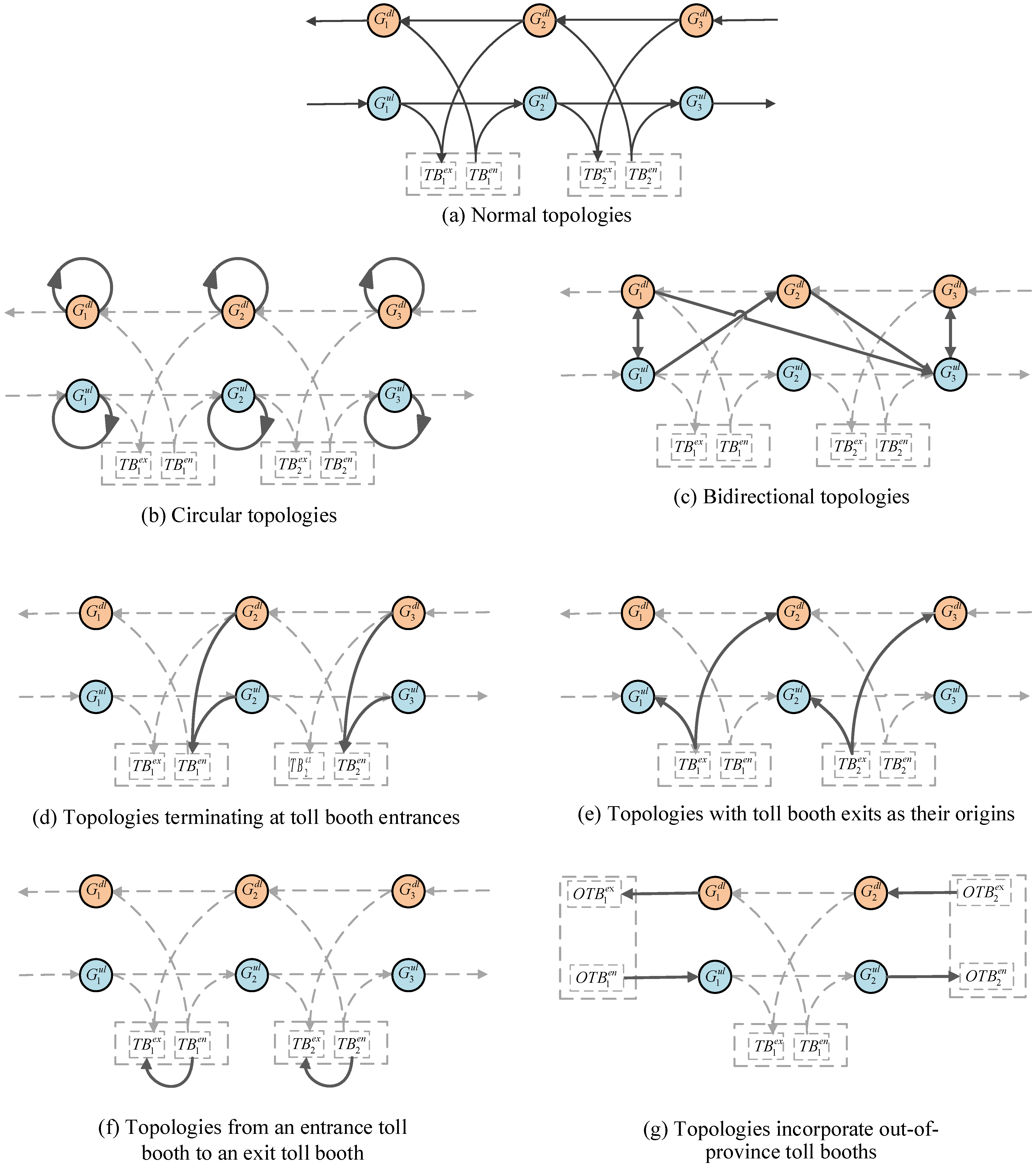
- Topologies not included in the ETC node set: In these topologies, the starting or ending point, or both, are not part of the node set. Thus, these topologies can be directly eliminated.
- Circular topologies: As depicted in Figure 2b, in these topologies, the start and end nodes are identical. This type of erroneous topology can be easily removed.
- Bidirectional topologies (Figure 2c): These candidate topologies feature nodes from the upward (downward) lane that directly reach nodes of the downward (upward) lane.
- Topologies terminating at toll booth entrances (Figure 2d): Similar to the case of topologies originating from exits, these topologies conclude at a toll booth entrance.
- Topologies originating from toll booth exits (Figure 2e): These topologies commence from a toll booth exit. However, in actual trajectories, toll booth exits typically appear at the end, hence such topologies do not exist.
- Topologies from an entrance toll booth to an exit toll booth (Figure 2f): These candidate topologies commence from an entrance toll booth and conclude at an exit toll booth. However, in actual trajectories, several gantries must be passed between the entrance and exit toll booths, rendering such topologies clearly erroneous and subject to direct elimination.
- Topologies incorporating out-of-province toll booths (Figure 2g): These topologies feature a toll booth node outside the province as the starting point or endpoint. In the figure, the toll station outside the province is OTB. Due to the presence of inter-provincial ETC transaction data in the actual dataset, topologies may contain nodes of out-of-province toll booths. These nodes can be easily identified as their toll booth names differ from those of in-province nodes, despite having identical IDs.
3.5. Feature Vector Modeling
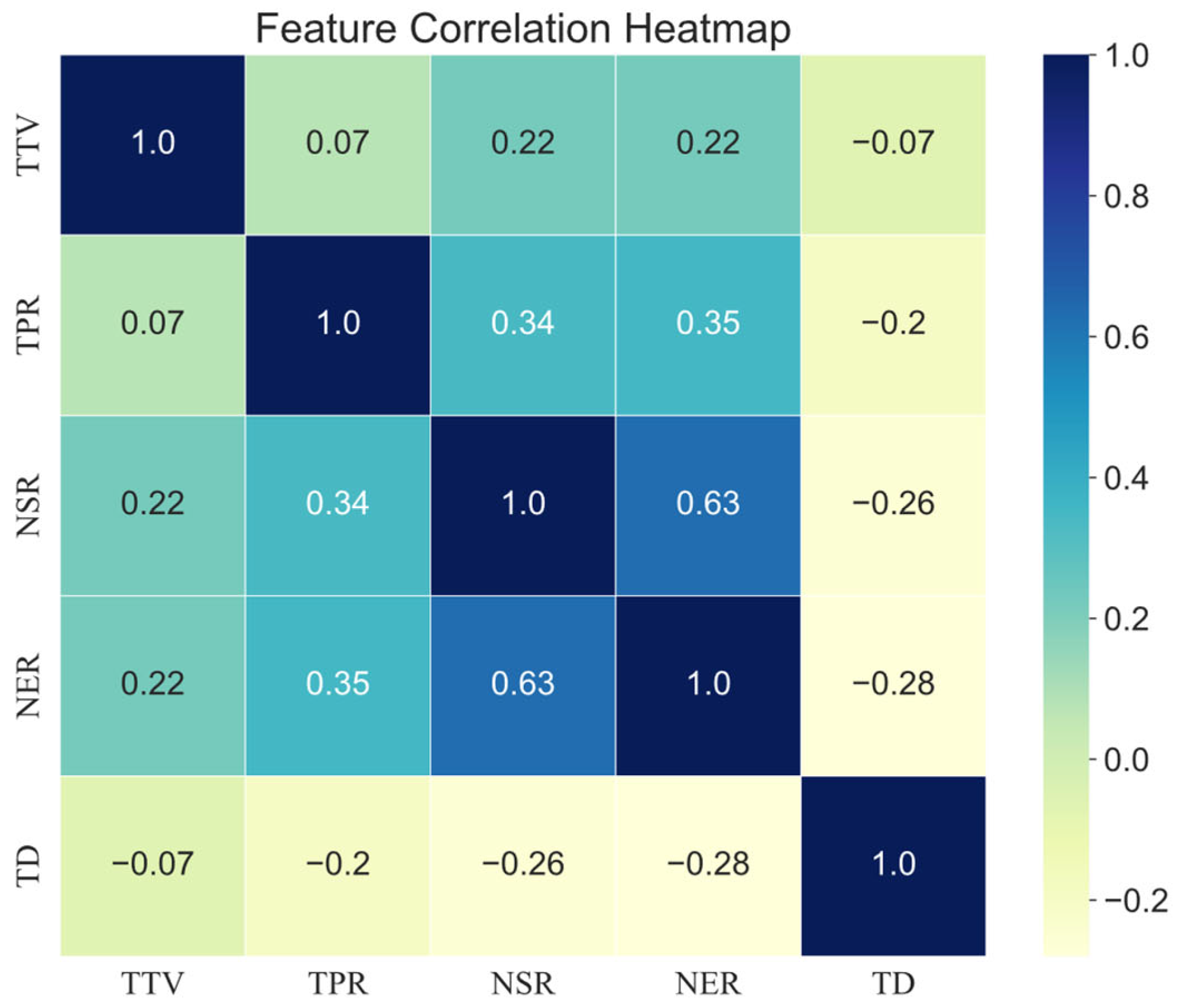
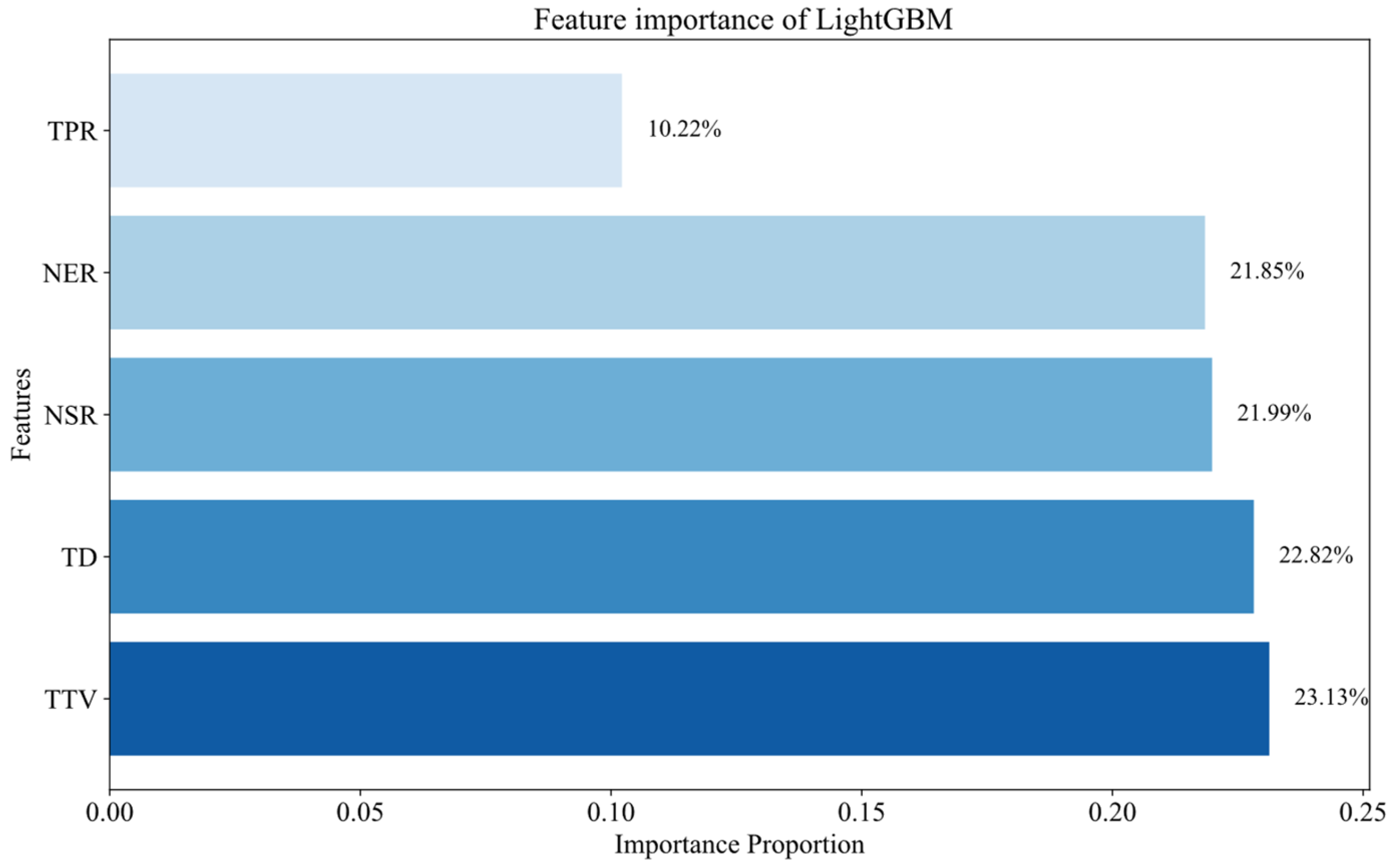
- Topology Traffic Volume (TTV): TTV, as a basic indicator of traffic flow, can reflect the importance of the topology in the traffic system. By analyzing this feature, we can understand the traffic differences in different topologies. TTV is calculated using Equation (1), where represents the number of trajectories of topology (a, b) on the i-th day, and N represents the number of days considered. In this study, N = 5.
- Topological Passage Rate (TPR): To calculate this feature, first, we calculate the number of trajectories containing both nodes a and b within a 5-day span, regardless of whether these two nodes are directly connected. We refer to this as the Coexisting Nodes Trajectory Volume (CNTV). The calculation formula for CNTV is shown in Equation (2), where represents the number of trajectories containing nodes A and B on the i-th day. The reason for choosing the TPR feature is that some topologies may have a large number of erroneous transactions or omissions, resulting in a high value of CNTV. By calculating the ratio of CNTV to TTV, we can more accurately assess the possibility of each topology in actual work. Then, we calculate the Topological Passage Rate, through the formula TPR = TTV/CNTV.
- Normalized Start Rate (NSR): In the actual high-speed ETC gantry topology, each starting node has 1 to 4 endpoints, and the rest of the topologies are likely to be generated by erroneous data. Therefore, by calculating the proportion of the traffic of candidate topology (a, b) in all the topologies starting from a, we can evaluate the possibility of this topology in actual work. Therefore, NSR is one of the crucial features for evaluating the existence probability of a topology. The computation formula for NSR is as shown in Equation (4), where M denotes the number of end nodes reached by the initial node a in the candidate topology.
- Normalized End Rate (NER): NER is the normalized rate of the end node, calculating the ratio of the traffic of topology (a, b) to the total traffic of all topologies ending at b. Since one end node may be connected to multiple start nodes, we need to consider all in-degree topologies of this end node. The calculation of NER is similar to that of NSR, but it is grouped by end node b. The computation formula for NSR is as shown in Equation (5).
3.6. Authenticity Verification and Accuracy Annotation of Candidate Topologies
3.7. Dynamic Generation Method of Highway ETC Gantry Topology Based on LightGBM
- Gradient Boosting: LightGBM is a model based on gradient boosting. Throughout the training process, it repetitively builds decision trees, striving to diminish the discrepancy between the predicted value, and the true value, y, at every step, thereby continually enhancing the prediction accuracy of the model. Its loss function is defined as . The iterative model can be expressed as:where represents the learning rate.
- Decision Tree Construction: Within LightGBM, the decision tree utilizes a depth-first approach for splitting, and it carries out efficient node splits according to the histogram of features. Additionally, LightGBM is capable of handling categorical features and employs a Gradient-based One-Side Sampling (GOSS) method [45] in feature selection, significantly enhancing training efficiency on high-dimensional data. GOSS is a sampling technique that preserves all large gradient samples and randomly selects a fraction of small gradient samples. This practice maintains the data’s distribution while reducing computational cost. The update of tree nodes is represented in a form approximated by the least squares method, as shown in Equation (8):where and denote the first and second order gradients, respectively. To maximize the model’s performance at each split, LightGBM seeks the optimal split point at every node division. The method of locating the best split point is achieved by maximizing the information gain. The specific calculation of information gain is as follows:where , , and are the optimal output values for each leaf node.
- Ensemble Prediction: After constructing N decision trees, LightGBM aggregates them for prediction. For a new input sample x, it is fed into each decision tree, and the obtained prediction result is the weighted average of all decision tree prediction results:
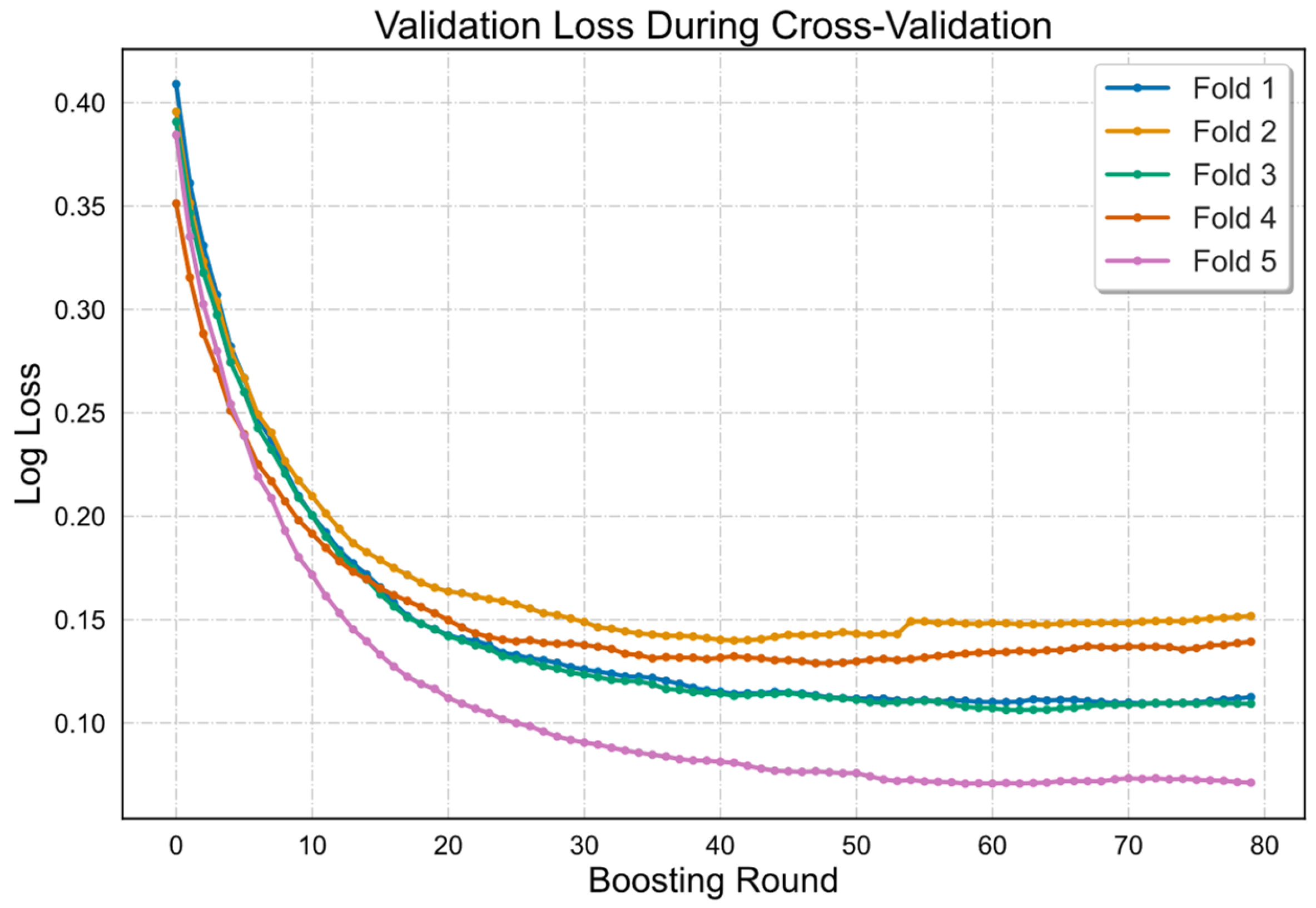
- Hyperparameter Optimization: A grid search is employed for hyperparameter optimization. The primary hyperparameters encompass the number of decision trees, the maximum depth of each tree, the learning rate, the number of features, etc. A parameter grid is defined, and the optimal hyperparameter combination is identified by iterating over potential parameter combinations.
4. Experiment and Results Analysis
4.1. Construction of Feature Vectors
4.2. Experimental Setup and Parameter Selection
4.3. Empirical Outcomes and Integrated Appraisal
4.4. Results of Gantry Topology Generation
5. Conclusions
Author Contributions
Funding
Data Availability Statement
Conflicts of Interest
Glossary
| Acronym | Full Form |
| AB | Adaptive Boosting |
| API | Application Programming Interface |
| DBSCAN | Density-Based Spatial Clustering of Applications with Noise |
| DT | Decision Tree |
| ETC | Electronic Toll Collection |
| GBDT | Gradient Boosting Decision Tree |
| GB | Gradient Boosting |
| GPC | Gaussian Process Classifier |
| GNSS | Global Navigation Satellite System |
| GPS | Global Positioning System |
| KDE | Kernel Density Estimation |
| KNN | k-Nearest Neighbors |
| LCSS | Longest Common Subsequence |
| LDA | Linear Discriminant Analysis |
| LightGBM | Light Gradient Boosting Machine |
| LR | Logistic Regression |
| MTC | Manual Toll Collection |
| NB | Naive Bayes Classifier |
| NSR | Normalized Start Rate |
| OBU | On-Board Unit |
| QDA | Quadratic Discriminant Analysis |
| RF | Random Forest |
| RSU | Road Side Unit |
| SGD | Stochastic Gradient Descent |
| SVM | Support Vector Machine |
| TD | Topology Distance |
| TTV | Topology Traffic Volume |
| XGB | XGBoost (Extreme Gradient Boosting) |
| 5 | 0.9763 |
Appendix A
| Parameter | Description | Value |
|---|---|---|
| C | Inverse regularization | 1 |
| class_weight | Class weights | None |
| dual | Dual formulation | False |
| fit_intercept | Add constant to function | True |
| intercept_scaling | For solver ‘liblinear’ | 1 |
| l1_ratio | Elastic-Net mixing | None |
| max_iter | Max iterations | 100 |
| multi_class | Multiclass option | Auto |
| n_jobs | CPU cores for parallel | None |
| penalty | Norm in penalization | L2 |
| random_state | Random number seed | None |
| solver | Optimization algorithm | Lbfgs |
| tol | Stopping criteria | 0.0001 |
| verbose | Verbose for liblinear | 0 |
| warm_start | Reuse previous solution | False |
| Parameter | Description | Value |
|---|---|---|
| priors | Prior probabilities | None |
| var_smoothing | Portion of the largest variance | 1 × 10⁻⁹ |
| priors | Prior probabilities | None |
| Parameter | Description | Value |
|---|---|---|
| covariance_estimator | Covariance estimator | None |
| n_components | Number of components | None |
| priors | Prior probabilities | None |
| shrinkage | Shrinkage parameter | None |
| solver | Solver for computation | Svd |
| store_covariance | If True, compute covariance | False |
| tol | Tolerance for stopping criteria | 0.0001 |
| Parameter | Description | Value |
|---|---|---|
| algorithm | Algorithm used | Auto |
| leaf_size | Leaf size | 30 |
| metric | Distance metric | Minkowski |
| metric_params | Metric params | None |
| n_jobs | Num of jobs | None |
| n_neighbors | Num of neighbors | 5 |
| p | Power parameter | 2 |
| weights | Weight function | Uniform |
| Parameter | Description | Value |
|---|---|---|
| ccp_alpha | Cost complexity pruning | 0 |
| class_weight | Class weights | None |
| criterion | Criterion to split | Gini |
| max_depth | Max depth of tree | None |
| max_features | Max features for split | None |
| max_leaf_nodes | Max leaf nodes | None |
| min_impurity_decrease | Node impurity decrease | 0 |
| min_samples_leaf | Min samples at leaf | 1 |
| min_samples_split | Min samples to split | 2 |
| min_weight_fraction_leaf | Min weight fraction | 0 |
| random_state | Random seed | None |
| splitter | Split strategy | Best |
| Parameter | Description | Value |
|---|---|---|
| bootstrap | Bootstrap samples | True |
| ccp_alpha | Cost complexity pruning | 0 |
| class_weight | Class weights | None |
| criterion | Split criterion | None |
| max_depth | Max tree depth | None |
| max_features | Max features | None |
| max_leaf_nodes | Max leaf nodes | None |
| max_samples | Max samples | None |
| min_impurity_decrease | Min impurity decrease | 0 |
| min_samples_leaf | Min samples at leaf | 1 |
| min_samples_split | Min samples to split | 2 |
| min_weight_fraction_leaf | Min weight fraction | 0 |
| n_estimators | Num of trees | 100 |
| n_jobs | Num of jobs | None |
| oob_score | OOB score | False |
| random_state | Random seed | None |
| verbose | Logging level | 0 |
| warm_start | Reuse previous solution | False |
| Parameter | Description | Value |
|---|---|---|
| C | Penalty parameter | 1 |
| break_ties | Break ties | False |
| cache_size | Cache size | 200 |
| class_weight | Class weights | None |
| coef0 | Kernel coef | 0 |
| decision_function_shape | Decision function | Ovr |
| degree | Kernel degree | 3 |
| gamma | Kernel coef | Scale |
| kernel | Kernel type | Rbf |
| max_iter | Max iterations | −1 |
| probability | Estimate prob | True |
| random_state | Random seed | None |
| shrinking | Use shrinking | True |
| tol | Tolerance | 0.001 |
| verbose | Verbose | False |
| Parameter | Description | Value |
|---|---|---|
| ccp_alpha | Pruning parameter | 0 |
| criterion | Split criterion | Friedman_mse |
| init | Initial estimator | None |
| learning_rate | Learning rate | 0.1 |
| loss | Loss function | Deviance |
| max_depth | Max depth | 3 |
| max_features | Max features | None |
| max_leaf_nodes | Max leaf nodes | None |
| min_impurity_decrease | Min impurity decrease | 0 |
| min_samples_leaf | Min samples at leaf | 1 |
| min_samples_split | Min samples to split | 2 |
| min_weight_fraction_leaf | Min weight fraction | 0 |
| n_estimators | Num of estimators | 100 |
| n_iter_no_change | Iterations no change | None |
| random_state | Random seed | None |
| subsample | Subsample fraction | 1 |
| tol | Tolerance | 0.0001 |
| validation_fraction | Validation fraction | 0.1 |
| verbose | Verbose | 0 |
| warm_start | Reuse previous solution | False |
| Parameter | Description | Value |
|---|---|---|
| algorithm | Algorithm type | Samme.r |
| base_estimator | Base estimator | None |
| learning_rate | Learning rate | 1 |
| n_estimators | Num of estimators | 50 |
| random_state | Random seed | None |
| verbose | Verbose for liblinear | 0 |
| warm_start | Reuse previous solution | False |
| Parameter | Description | Value |
|---|---|---|
| use_label_encoder | Use label encoder | False |
| enable_categorical | Categorical data | False |
| eval_metric | Evaluation metric | Logloss |
| objective | Objective function | Binary:logistic |
| n_estimators | Num of estimators | 100 |
| Parameter | Description | Value |
|---|---|---|
| priors | Class priors | None |
| reg_param | Regularization | 0 |
| store_covariance | Store covariance | False |
| tol | Tolerance | 0.0001 |
| Parameter | Description | Value |
|---|---|---|
| copy_X_train | Copy training data | True |
| kernel | Kernel function | None |
| max_iter_predict | Max iterations | 100 |
| multi_class | Multi-class strategy | One_vs_rest |
| n_jobs | Num of jobs | None |
| n_restarts_optimizer | Num of restarts | 0 |
| optimizer | Optimizer | Fmin_l_bfgs_b |
| random_state | Random seed | None |
| warm_start | Reuse previous solution | False |
| Parameter | Description | Value |
|---|---|---|
| alpha | Regularization param | 0.0001 |
| average | Average coef | False |
| class_weight | Class weights | |
| early_stopping | Early stopping | False |
| epsilon | Epsilon | 0.1 |
| eta0 | Initial learning rate | 0 |
| fit_intercept | Fit intercept | True |
| l1_ratio | L1 ratio | 0.15 |
| learning_rate | Learning rate | Optimal |
| loss | Loss function | Hinge |
| max_iter | Max iterations | 1000 |
| n_iter_no_change | Iterations no change | 5 |
| n_jobs | Num of jobs | None |
| penalty | Penalty | L2 |
| power_t | Power t | 0.5 |
| random_state | Random seed | None |
| shuffle | Shuffle | True |
| tol | Tolerance | 0.001 |
| validation_fraction | Validation fraction | 0.1 |
| verbose | Verbose | 0 |
| warm_start | Reuse previous solution | False |
| Parameter | Description | Value |
|---|---|---|
| C | Regularization param | 1 |
| class_weight | Class weights | None |
| dual | Dual formulation | True |
| fit_intercept | Fit intercept | True |
| intercept_scaling | Intercept scaling | 1 |
| loss | Loss function | Squared_hinge |
| max_iter | Max iterations | 1000 |
| multi_class | Multi-class strategy | None |
| penalty | Penalty | L2 |
| random_state | Random seed | None |
| tol | Tolerance | 0.0001 |
References
- Ministry of Transport, National Development and Reform Commission, Ministry of Finance. Notice on Issuing the Implementation Plan for the Full Promotion of Differentiated Toll Collection on Highways. Jiaogongluhan No. 228. 2021. Available online: https://www.gov.cn/zhengce/zhengceku/2021-06/15/content_5617919.htm (accessed on 30 July 2023).
- Cai, Q.; Yi, D.; Zou, F.; Wang, W.; Luo, G.; Cai, X. An Arch-Bridge Topology-Based Expressway Network Structure and Automatic Generation. Appl. Sci. 2023, 13, 5031. [Google Scholar] [CrossRef]
- Fujian Provincial State-Owned Assets Supervision and Administration Commission. Fujian: ETC Usage Rate Ranks First in the Country. 12 December 2019. Available online: http://www.sasac.gov.cn/n2588025/n2588129/c13072896/content.html (accessed on 30 July 2023).
- Amap. Web Service API. Amap API. Available online: https://lbs.amap.com/api/webservice/summary/ (accessed on 27 July 2023).
- QGIS Development Team. QGIS Desktop User Guide/Manual (QGIS 3.28). Available online: https://docs.qgis.org/3.28/en/docs/user_manual/ (accessed on 27 July 2023).
- Kass, M.; Witkin, A.; Terzopoulos, D. Snakes: Active contour models. Int. J. Comput. Vis. 1988, 1, 321–331. [Google Scholar] [CrossRef]
- Péteri, R.; Ranchin, T. Extraction of network-like structures using a multiscale representation. IEEE Geosci. Remote Sens. Lett. 2005, 2, 402–406. [Google Scholar]
- Laptev, I.; Caputo, B.; Schuldt, C.; Lindeberg, T. Local velocity-adapted motion events for spatio-temporal recognition. Comput. Vis. Image Underst. 2004, 108, 207–229. [Google Scholar] [CrossRef]
- Gruen, A.; Li, H. Linear feature extraction with dynamic programming and Globally Least Squares. ISPRS J. Photogramm. Remote Sens. 1995, 50, 23–30. [Google Scholar]
- Mokhtarzade, M.; Zoej, M.V. Road detection from high-resolution satellite images using artificial neural networks. Int. J. Appl. Earth Obs. Geoinf. 2007, 9, 32–40. [Google Scholar] [CrossRef]
- Yager, K.; Sowmya, A. Road detection from aerial images using SVMs. Mach. Vis. Appl. 2008, 19, 261–274. [Google Scholar]
- Mnih, V.; Hinton, G.E. Learning to Detect Roads in High-Resolution Aerial Images; Springer: Berlin/Heidelberg, Germany, 2010; pp. 210–223. [Google Scholar]
- He, K.; Zhang, X.; Ren, S.; Sun, J. Deep residual learning for image recognition. In Proceedings of the IEEE Conference on Computer Vision and Pattern Recognition, Las Vegas, NV, USA, 27–30 June 2016; pp. 770–778. [Google Scholar]
- Saito, S.; Yamashita, T.; Aoki, Y. Multiple object extraction from aerial imagery with convolutional neural networks. Electron. Imaging 2016, 2016, 1–9. [Google Scholar] [CrossRef]
- Long, J.; Shelhamer, E.; Darrell, T. Fully convolutional networks for semantic segmentation. In Proceedings of the IEEE Conference on Computer Vision and Pattern Recognition, Boston, MA, USA, 7–12 June 2015; pp. 3431–3440. [Google Scholar]
- Maggiori, E.; Tarabalka, Y.; Charpiat, G.; Alliez, P. Fully convolutional neural networks for remote sensing image classification. In Proceedings of the 2016 IEEE International Geoscience and Remote Sensing Symposium (IGARSS), Beijing, China, 10–15 June 2016; pp. 5071–5074. [Google Scholar]
- Ševo, I.; Avramović, A. Convolutional Neural Network Based Automatic Object Detection on Aerial Images. IEEE Geosci. Remote Sens. Lett. 2016, 13, 740–744. [Google Scholar] [CrossRef]
- Volpi, M.; Tuia, D. Dense Semantic Labeling of Subdecimeter Resolution Images with Convolutional Neural Networks. IEEE Trans. Geosci. Remote Sens. 2017, 55, 881–893. [Google Scholar] [CrossRef]
- Maggiori, E.; Tarabalka, Y.; Charpiat, G.; Alliez, P. Convolutional neural networks for large-scale remote-sensing image classification. IEEE Trans. Geosci. Remote Sens. 2017, 55, 645–657. [Google Scholar] [CrossRef]
- Keramitsoglou, I.; Kontoes, C.; Sifakis, N.; Konstantinidis, P.; Fitoka, E. Deep learning for operational land cover mapping using Sentinel-2 data. J. Appl. Remote Sens. 2020, 14, 014503. [Google Scholar]
- Wagstaff, K.; Cardie, C.; Rogers, S.; Schroedl, S. Constrained k-means clustering with background knowledge. In Proceedings of the Eighteenth International Conference on Machine Learning (ICML), San Francisco, CA, USA, 28 June–1 July 2001; Volume 1, pp. 577–584. [Google Scholar]
- Schroedl, S.; Wagstaff, K.; Rogers, S.; Langley, P.; Wilson, C. Mining GPS traces for map refinement. Data Min. Knowl. Discov. 2004, 9, 59–87. [Google Scholar] [CrossRef]
- Worrall, S.; Nebot, E. Automated process for generating digitised maps through GPS data compression. In Proceedings of the Australasian Conference on Robotics and Automation (ACRA), Brisbane, Australia, 10–12 December 2007; Volume 6. [Google Scholar]
- Sasaki, Y.; Yu, J.; Ishikawa, Y. Road segment interpolation for incomplete road data. In Proceedings of the IEEE International Conference on Big Data and Smart Computing, Kyoto, Japan, 27 February–2 March 2019; pp. 1–8. [Google Scholar]
- Edelkamp, S.; Schrödl, S. Route planning and map inference with global positioning traces. In Computer Science in Perspective; Springer: Berlin/Heidelberg, Germany, 2003; pp. 128–151. [Google Scholar]
- Chen, C.; Lu, C.; Huang, Q.; Yang, Q.; Gunopulos, D.; Guibas, L. City-scale map creation and updating using GPS collections. In Proceedings of the 22nd ACM SIGKDD International Conference on Knowledge Discovery and Data Mining, San Francisco, CA, USA, 13–17 August 2016; pp. 1465–1474. [Google Scholar]
- Huang, J.; Zhang, Y.; Deng, M.; He, Z. Mining crowdsourced trajectory and geo-tagged data for spatial-semantic road map construction. Trans. GIS 2022, 26, 735–754. [Google Scholar] [CrossRef]
- Silverman, B.W. Density Estimation for Statistics and Data Analysis; Routledge: Abingdon, UK, 2018. [Google Scholar]
- Fu, Z.; Fan, L.; Sun, Y.; Tian, Z. Density adaptive approach for generating road network from GPS trajectories. IEEE Access 2020, 8, 51388–51399. [Google Scholar] [CrossRef]
- Uduwaragoda, E.; Perera, A.S.; Dias, S.A.D. Generating lane level road data from vehicle trajectories using kernel density estimation. In Proceedings of the 16th International IEEE Conference on Intelligent Transportation Systems (ITSC 2013), The Hague, The Netherlands, 6–9 October 2013; pp. 384–391. [Google Scholar]
- Kuntzsch, C.; Sester, M.; Brenner, C. Generative models for road network reconstruction. Int. J. Geogr. Inf. Sci. 2016, 30, 1012–1039. [Google Scholar] [CrossRef]
- Neuhold, R.; Haberl, M.; Fellendorf, M.; Pucher, G.; Dolancic, M.; Rudigier, M.; Pfister, J. Generating a lane-specific transportation network based on floating-car data. In Advances in Human Aspects of Transportation; Springer: Cham, Switzerland, 2017; pp. 1025–1037. [Google Scholar]
- Huang, Y.; Xiao, Z.; Yu, X.; Wang, D. Road network construction with complex intersections based on sparsely sampled private car trajectory data. ACM Trans. Knowl. Discov. Data (TKDD) 2019, 13, 1–28. [Google Scholar] [CrossRef]
- Deng, M.; Huang, J.; Zhang, Y.; Liu, H.; Tang, L.; Tang, J.; Yang, X. Generating urban road intersection models from low-frequency GPS trajectory data. Int. J. Geogr. Inf. Sci. 2018, 32, 2337–2361. [Google Scholar] [CrossRef]
- Wu, J.; Zhu, Y.; Ku, T.; Wang, L. Detecting Road Intersections from Coarse-gained GPS Traces Based on Clustering. J. Comput. 2013, 8, 2959–2965. [Google Scholar] [CrossRef]
- Xie, X.; Philips, W. Road intersection detection through finding common sub-tracks between pairwise GNSS traces. ISPRS Int. J. Geo-Inf. 2017, 6, 311. [Google Scholar] [CrossRef]
- Fathi, A.; Krumm, J. Detecting road intersections from GPS traces. In Proceedings of the International Conference on Geographic Information Science, Zurich, Switzerland, 14–17 September 2010; Springer: Berlin/Heidelberg, Germany, 2010; pp. 56–69. [Google Scholar]
- Karagiorgou, S.; Pfoser, D. On vehicle tracking data-based road network generation. In Proceedings of the 20th International Conference on Advances in Geographic Information Systems, Redondo Beach, CA, USA, 6–9 November 2012; pp. 89–98. [Google Scholar]
- Pu, M.; Mao, J.; Du, Y.; Shen, Y.; Jin, C. Road intersection detection based on direction ratio statistics analysis. In Proceedings of the 2019 20th IEEE International Conference on Mobile Data Management (MDM), Hong Kong, China, 10–13 June 2019; pp. 288–297. [Google Scholar]
- Zhao, L.; Mao, J.; Pu, M.; Liu, G.; Jin, C.; Qian, W.; Zhou, A.; Wen, X.; Hu, R.; Chai, H. Automatic calibration of road intersection topology using trajectories. In Proceedings of the 2020 IEEE 36th International Conference on Data Engineering (ICDE), Kuala Lumpur, Malaysia, 20–24 April 2020; pp. 1633–1644. [Google Scholar]
- Qing, R.; Liu, Y.; Zhao, Y.; Liao, Z.; Liu, Y. Using feature interaction among GPS Data for road intersection detection. In Proceedings of the 2nd International Workshop on Human-Centric Multimedia Analysis, Cheng Du, China, 20–24 October 2021; pp. 31–37. [Google Scholar]
- Liu, Y.; Qing, R.; Zhao, Y.; Liao, Z. Road Intersection Recognition via Combining Classification Model and Clustering Algorithm Based on GPS Data. ISPRS Int. J. Geo-Inf. 2022, 11, 487. [Google Scholar] [CrossRef]
- Ministry of Transport of the People’s Republic of China. Vehicle Classification of the Toll for Highway (JT/T 489-2019). 2019. Available online: https://jtst.mot.gov.cn/kfs/file/read/0de9ee528422ee3a99ff87b1c1295e8e (accessed on 30 July 2023).
- Ke, G.; Meng, Q.; Finley, T.; Wang, T.; Chen, W.; Ma, W.; Ye, Q.; Liu, T.Y. Lightgbm: A highly efficient gradient boosting decision tree. Adv. Neural Inf. Process. Syst. 2017, 30, 3149–3157. [Google Scholar] [CrossRef]
- Meng, Q.; Ke, G.; Wang, T.; Chen, W.; Ye, Q.; Ma, Z.M.; Liu, T.Y. A communication-efficient parallel algorithm for decision tree. Adv. Neural Inf. Process. Syst. 2016, 29, 1279–1287. [Google Scholar] [CrossRef]

| Index | Field Name | Field Properties | Example |
|---|---|---|---|
| 1 | GantryID | gantry id number | 340E11 |
| 2 | GantryName | gantry name | Jinhai to Nanzhou |
| 3 | GantryType | gantry type | 2 |
| 4 | GantryCor | gantry geographic coordinates | (119.308, 25.888) |
| 5 | OBUid | vehicular identifiers | 1452687261 |
| 6 | PassID | journey identifiers | 0142***561 |
| 7 | TradeTime | transactional timestamps | 2021/6/1 12:00:00 |
| 8 | ErrorCode | transaction error codes | 1 |
| Index | Field Name | Field Properties | Example |
|---|---|---|---|
| 1 | EnBoothID | entrance booth id number | 2100 |
| 2 | EnBoothName | entrance booth name | Jinhai toll booth |
| 3 | EnBoothType | entrance booth type | 0 |
| 4 | EnBoothCor | entrance booth geographic coordinates | (118.318, 26.778) |
| 5 | OBUid | vehicular identifiers | 1452687261 |
| 6 | PassID | journey identifiers | 0142***561 |
| 7 | TradeTime | transactional timestamps | 2021/6/1 12:00:00 |
| 8 | ErrorCode | transaction error codes | 1 |
| Index | Field Name | Field Properties | Example |
|---|---|---|---|
| 1 | ExBoothID | exit booth id number | 2100 |
| 2 | ExBoothName | exit booth name | Jinhai toll booth |
| 3 | ExBoothType | exit booth type | 1 |
| 4 | ExBoothCor | exit booth geographic coordinates | (118.316, 26.767) |
| 5 | OBUid | vehicular identifiers | 1452687261 |
| 6 | PassID | journey identifiers | 0142***561 |
| 7 | TradeTime | transactional timestamps | 2021/6/1 12:00:00 |
| 8 | ErrorCode | transaction error codes | 1 |
| Index | Field Name | Field Properties | Example |
|---|---|---|---|
| 1 | NodeID | node id number | 34E102 |
| 2 | NodeName | node name | Jinhai toll booth |
| 3 | NodeType | node type | 1 |
| 4 | NodeCor | node geographic coordinates | (118.456, 26.657) |
| 5 | TradeTime | transactional timestamps | 2021/6/1 12:00:00 |
| 6 | OBUid | vehicular identifiers | 1452687261 |
| 7 | PassID | journey identifiers | 0142***561 |
| PassID | Index | Transit Node Transaction Time | Transit Node ID | Transit Node Name | Transit Node Type | Transit Topological Segment |
|---|---|---|---|---|---|---|
| 0142***561 | 1 | 2021-06-01 08:00:00 | 2100EN | Zhongnan Jinghai Booth | 0 | |
| 2 | 2021-06-01 09:00:00 | 350001 | Jinghai to Xijin Hub | 2 | 2100EN–350001 | |
| 3 | 2021-06-01 10:00:00 | 350003 | Xijin Hub to Dongcheng | 2 | 350001–350003 | |
| 4 | 2021-06-01 11:00:00 | 350005 | Dongcheng to Xiyu Hub | 2 | 350003–350005 | |
| 5 | 2021-06-01 12:00:00 | 350007 | Xiyu Hub to Nancheng | 2 | 350005–350007 | |
| 6 | 2021-06-01 13:00:00 | 2200EX | Zhongnan Nancheng Booth | 1 | 350007–2200EX |
| Category | Number of Nodes |
|---|---|
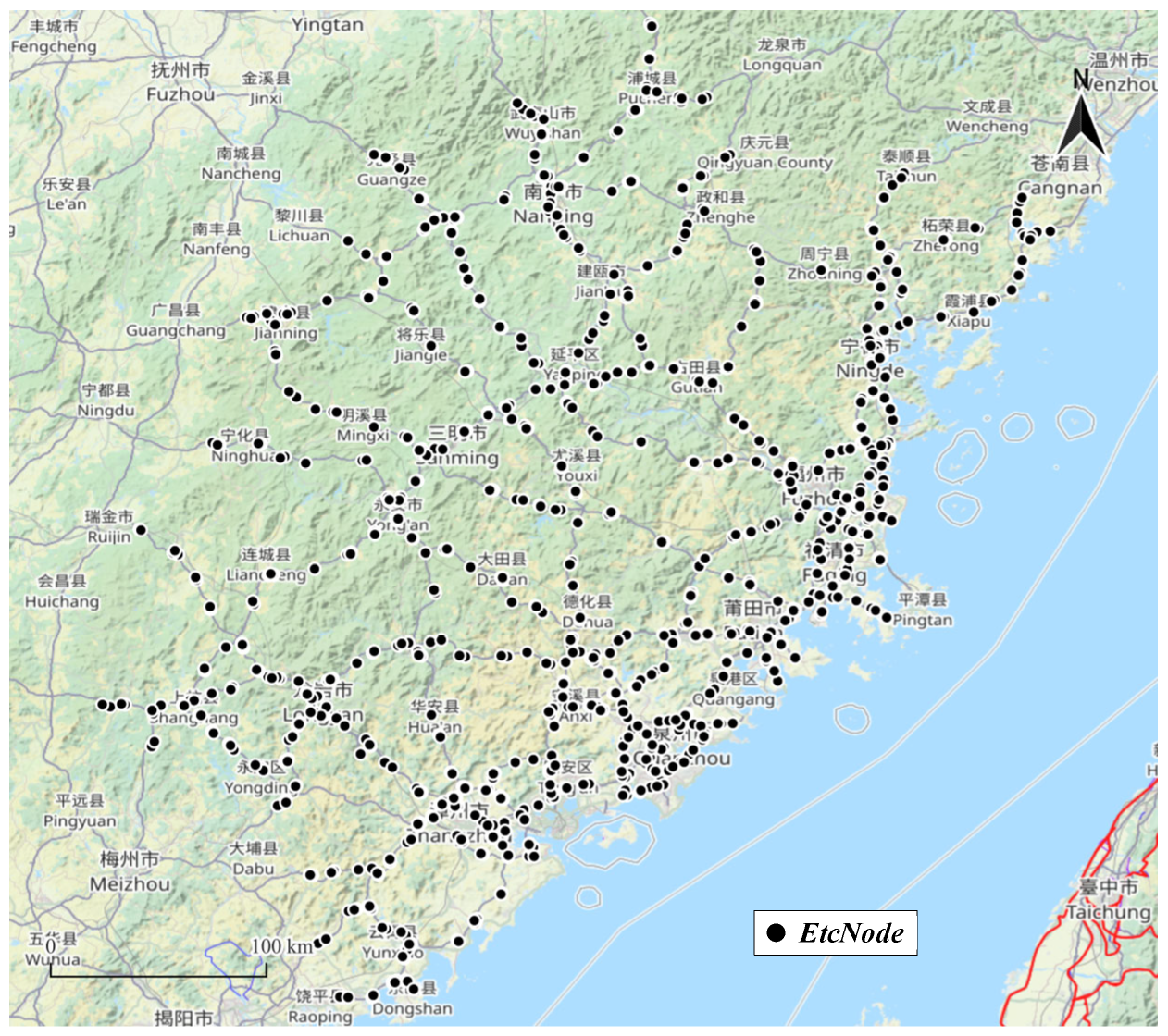
| Gantry Nodes | 1051 |
| Entry Toll Booth Nodes | 378 |
| Exit Toll Booth Nodes | 376 |
| Total | 1805 |
| Index | Field Name | Field Properties | Example |
|---|---|---|---|
| 1 | Topology | topology array | [‘350E01’, ‘350E03’] |
| 2 | StartID | start node id | 350E01 |
| 3 | EndID | end node id | 350E03 |
| 4 | StartName | start node name | Jinhai to Nanzhou |
| 5 | EndName | end node name | Nanzhou to Xicheng |
| 6 | StartType | start node type | 2 |
| 7 | EneType | end node type | 2 |
| 8 | StartCor | start node geographic coordinate | (118.2434, 24.6884) |
| 9 | EndCor | end node geographic coordinate | (118.4107, 24.7195) |
| 10 | TrafficVolume | topology traffic volume | 257,396 |
| 11 | TopologyDistance | topology route distance | 18,561 (m) |
| Candidate Topo | TTV | TPR | NSR | NER | TD | Label |
|---|---|---|---|---|---|---|
| [‘67**EN’, ‘34**19’] | 6091 | 0.99918 | 0.2431 | 0.1157 | 1357 | 1 |
| [‘67**EN’, ‘35**03’] | 1212 | 0.999176 | 0.212 | 0.4994 | 13723 | 0 |
| [‘34**07’, ‘34**0B’] | 1199 | 0.999167 | 0.1612 | 0.3223 | 1357 | 1 |
| [‘35**62’, ‘35**5F’] | 314 | 0.996825 | 0.397 | 0.139 | 1802 | 1 |
| [‘35**04’, ‘35**11’] | 933 | 0.996795 | 0.1447 | 0.6839 | 1346 | 1 |
| [‘34**15’, ‘34**19’] | 2788 | 0.996782 | 0.0281 | 0.1053 | 1545 | 1 |
| [‘79**EN’, ‘35**23’] | 128 | 0.711111 | 0.0242 | 0.0006 | 2554 | 0 |
| [‘35**13’, ‘35**23’] | 211 | 0.710438 | 0.0179 | 0.0012 | 6955 | 0 |
| [‘34**07’, ‘35**5F’] | 571 | 0.710199 | 0.1008 | 0.0049 | 4523 | 0 |
| [‘64**EN’, ‘34**19’] | 236 | 0.571429 | 0.0977 | 0.278 | 3254 | 1 |
| [‘47**EN’, ‘34**19’] | 6091 | 0.99918 | 0.2431 | 0.1157 | 1357 | 1 |
| [‘34**EN’, ‘35**03’] | 1212 | 0.999176 | 0.212 | 0.4994 | 13723 | 0 |
| Parameter Categories | Parameter | Search Range | Step Size | Optimal Value |
|---|---|---|---|---|
| general parameters | n_estimators | [10, 500] | 10 | 80 |
| learning_rate | [0.1, 0.01, 0.001] | - | 0.1 | |
| core parameters | max_depth | [3, 10] | 1 | 5 |
| num_leaves | [2, 50] | 1 | 7 | |
| min_child_samples | [5, 50] | 5 | 5 | |
| min_child_weight | [0.001, 0.01, 0.1] | - | 0.001 | |
| min_split_gain | [0, 0.1, 0.5] | - | 0 | |
| regularization parameters | reg_alpha | [0, 0.1, 0.5] | - | 0 |
| reg_lambda | [0, 0.1, 0.5] | - | 0 | |
| sampling parameters | subsample | [0.5, 0.9] | 0.2 | 0.5 |
| colsample_bytree | [0.5, 0.9] | 0.2 | 0.5 | |
| subsample_freq | [1, 5] | 2 | 3 |
| Model | Accuracy | Precision | Recall | F1-Score |
|---|---|---|---|---|
| LR | 0.8239 | 0.8918 | 0.8835 | 0.8877 |
| NB | 0.8705 | 0.8717 | 0.9797 | 0.9225 |
| LDA | 0.9403 | 0.9310 | 0.9982 | 0.9634 |
| KNN | 0.8574 | 0.8625 | 0.9741 | 0.9149 |
| DT | 0.9549 | 0.9688 | 0.9741 | 0.9714 |
| RF | 0.9651 | 0.9624 | 0.9945 | 0.9782 |
| SVM | 0.8617 | 0.8517 | 0.9982 | 0.9191 |
| GB | 0.9636 | 0.9624 | 0.9926 | 0.9773 |
| AB | 0.9578 | 0.9571 | 0.9908 | 0.9737 |
| XGB | 0.9651 | 0.9691 | 0.9871 | 0.9780 |
| LightGBM | 0.9709 | 0.9668 | 0.9982 | 0.9822 |
| QDA | 0.9607 | 0.9606 | 0.9908 | 0.9754 |
| GPC | 0.4032 | 0.9456 | 0.2569 | 0.4041 |
| SGD | 0.7365 | 0.9186 | 0.7301 | 0.8136 |
| Linear SVM | 0.7875 | 0.7875 | 1.0000 | 0.8811 |
| Fold | Accuracy | Precision | Recall | F1-Score |
|---|---|---|---|---|
| 1 | 0.9672 | 0.9631 | 0.9978 | 0.9801 |
| 2 | 0.9599 | 0.9614 | 0.9911 | 0.9760 |
| 3 | 0.9599 | 0.9577 | 0.9956 | 0.9763 |
| 4 | 0.9563 | 0.9667 | 0.9831 | 0.9748 |
| 5 | 0.9763 | 0.9803 | 0.9912 | 0.9857 |
Disclaimer/Publisher’s Note: The statements, opinions and data contained in all publications are solely those of the individual author(s) and contributor(s) and not of MDPI and/or the editor(s). MDPI and/or the editor(s) disclaim responsibility for any injury to people or property resulting from any ideas, methods, instructions or products referred to in the content. |
© 2023 by the authors. Licensee MDPI, Basel, Switzerland. This article is an open access article distributed under the terms and conditions of the Creative Commons Attribution (CC BY) license (https://creativecommons.org/licenses/by/4.0/).
Share and Cite
Zou, F.; Wang, W.; Cai, Q.; Guo, F.; Shi, R. Dynamic Generation Method of Highway ETC Gantry Topology Based on LightGBM. Mathematics 2023, 11, 3413. https://doi.org/10.3390/math11153413
Zou F, Wang W, Cai Q, Guo F, Shi R. Dynamic Generation Method of Highway ETC Gantry Topology Based on LightGBM. Mathematics. 2023; 11(15):3413. https://doi.org/10.3390/math11153413
Chicago/Turabian StyleZou, Fumin, Weihai Wang, Qiqin Cai, Feng Guo, and Rouyue Shi. 2023. "Dynamic Generation Method of Highway ETC Gantry Topology Based on LightGBM" Mathematics 11, no. 15: 3413. https://doi.org/10.3390/math11153413
APA StyleZou, F., Wang, W., Cai, Q., Guo, F., & Shi, R. (2023). Dynamic Generation Method of Highway ETC Gantry Topology Based on LightGBM. Mathematics, 11(15), 3413. https://doi.org/10.3390/math11153413


