Abstract
Time dilation (TD) is a principal concept in the special theory of relativity (STR). The Einstein TD formula is the relation between the proper time measured in a moving frame of reference with velocity v and the dilated time t measured by a stationary observer. In this paper, an integral approach is firstly presented to rededuce the Einstein TD formula. Then, the concept of TD is introduced and examined in view of the fractional calculus (FC) by means of the Caputo fractional derivative definition (CFD). In contrast to the explicit standard TD formula, it is found that the fractional TD (FTD) is governed by a transcendental equation in terms of the hyperbolic function and the fractional-order . For small v compared with the speed of light c (i.e., ), our results tend to Newtonian mechanics, i.e., . For v comparable to c such as , our numerical results are compared with the experimental ones for the TD of the muon particles . Moreover, the influence of the arbitrary-order on the FTD is analyzed. It is also declared that at a specific , there is an agreement between the present theoretical results and the corresponding experimental ones for the muon particles .
MSC:
83A05; 34A34
1. Introduction
Fractional calculus (FC) is an extension of classical calculus (CC). FC has been used to generalize/investigate numerous physical phenomena [1,2,3]. In the literature, various engineering and physical models have been studied in view of FC. Narahari et al. [4] applied FC to the dynamics of the fractional oscillator. In [5], Sebaa et al. investigated the ultrasonic wave propagation in human cancelous bone in FC. Tarasov [6] discussed the fractional Heisenberg equation. The fractional-order differential equation model of HIV infection has been analyzed by Ding and Yea [7]. Wang et al. [8] introduced the time-fractional diffusion equation and its applications in fractional quantum mechanics. Other interesting models in different areas have been considered by Song et al. [9], Gomez-Aguilara et al. [10], Machado et al. [11], Garcia [12], Machado [13], and Liaqat et al. [14].
In addition, Ebaid [15] and Ebaid et al. [16] analyzed the fractional model describing the projectile motion by means of the Caputo fractional derivative (CFD). Moreover, Ebaid et al. [16] compared their results utilizing the CFD with the available experimental data, while Ahmed et al. [17] imposed the Riemann–Liouville fractional derivative (RLFD) to analyze the same problem. In Refs. [17,18], the authors investigated the astronomical model of the surface brightness in the Milky Way utilizing the CFD. Furthermore, it was shown in Ref. [19] that the exact solution of such a model is available using an analytical approach. El-Zahar et al. [20] extended the application of the RLFD to solve the same astronomical model in a closed form. In Refs. [21,22,23,24,25,26,27,28,29], several ideas and applications of FC have been introduced. Very recently, Aljohani et al. [30] studied the fractional chlorine transport model, while Ebaid and Al-Jeaid [31] obtained the dual solution for a class of engineering oscillatory problems via the RLFD.
The concept of time dilation (TD) may have appeared with the advent of the special theory of relativity; see Refs. [32,33]. According to this concept, our understanding of all physical phenomena that depend on the velocity of the observer has changed. Thus, we have now what is called relativistic mechanics, which leads to the corresponding results in the classical Newtonian mechanics in the case of small relative velocity of the observer compared with the speed of light. A simple derivation of the TD formula has been introduced in Ref. [34]. Indeed, empirical science has proven the truth of Einstein’s predictions about time dilation. In fact, the validity of Einstein’s TD formula has been demonstrated by conducting a variety of experiments. Consequently, relativistic mechanics has become the cornerstone of modern physics, especially when studying the decay of particles that move with velocities close to the speed of light, such as muons.
In this regard, the CERN experiment [35] revealed that the empirical results are in agreement with the theoretical ones with 95% accuracy. But a question remains open: Where did the rest of the accuracy (i.e., 5%) go? In other words, why do we not find complete agreement between CERN’s results and Einstein’s TD formula? Perhaps the answer lies in rededucing the TD formula through considering another approach like the FC concept, as an example. This is the main motivation to put forward the current study. Therefore, this issue will be rebranded in light of FC. To achieve this target, we rededuce the Einstein standard TD formula using the concept of integration in the CC. Hence, a proposed generalization of such an integral formula is addressed by incorporating FC. By this, the concept of TD will be extended/generalized, and thus, a fractional TD formula (FTD) is to be derived. Since the fractional integral depends mainly on an arbitrary order , the influence of on the results is addressed. Finally, several comparisons with the standard TD formula are performed, as well as with the experimental results.
2. Concepts of the FC
The Riemann–Liouville fractional integral of order is defined as [1,2,3]:
Let denote the order of the derivative in such a way that . Then, the Caputo fractional derivative (CFD) of a function is defined by [1,2,3]
Particularly, for , the CFD of a function is defined by
One of the main important properties of the CFD is given by
where and are the Gamma functions. For , we have from Equation (4) that
The hypergeometric function is defined by the integral:
The last two relations are used later to derive the formula of TD in view of FC, utilizing the CFD, and are symbolized by FTD. However, the following lemmas facilitate the derivation of the FTD formula.
Lemma 1.
For , we have
Proof.
Lemma 2.
For , we have the integral:
3. Derivation of Standard TD Formula via Integral Technique
Consider a photon projected vertically toward the mirror in Figure 1. A stationary observer will find the time taken by the photon to cut the distances DA (up) and AD (down after reflection) as
For another nonstationary observer moving with a relative velocity v in the x-direction, the path of the photon is seen as the diagonal OA (before reflection) and then the diagonal AB (just after reflection). Accordingly, the time t measured by the nonstationary observer is
where OA = AB. Based on the geometry of Figure 1, we have the following coordinates for the points A, D, and B
The relation between t and was obtained by Einstein as and known as Einstein’s TD formula. It was basically derived from the fact that the triangle OAD is a right-angled triangle. This relation is deduced in this section via integral formula. The first step is to express the length of the hypotenuse OA in the integral form:
where describes the straight line passing through the origin O = (0, 0) and the point A = .
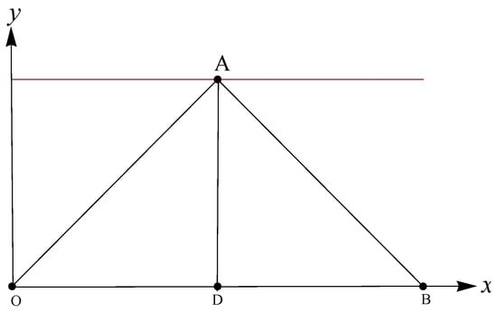
Figure 1.
Geometrical figure for the derivation of the standard TD formula via an integral approach.
The equation of the straight line OA is given by
or
Hence, Equation (20) gives
Substituting (23) into (18) yields
Solving this equation for t, we obtain
which is the Einstein’s TD formula in the special theory of relativity (STR).
4. The TD in FC (FTD)
In view of the FC, the first-order derivative can be replaced by the generalized derivative of arbitrary-order (). It may be important here to refer to the fact that the present CFD is chosen just to give an example for the application of fractional derivative operators to extend the concept of TD in FC. On occasion, other fractional derivative operators such as the RLFD [20] and the conformable derivative [21] can be utilized in separate works. Accordingly, a generalized form of Equation (20) may be defined by
Since , then
or
where
Inserting (28) into (26) gives
Suppose that
it then follows from (30) that
When comparing the integral in the right-hand side of Equation (32) with the integral I in (11), we find
Therefore,
Consequently, Equation (32) becomes
From (18) and (35), we obtain
The last equation can also be written in terms of t and as
It is noted from Equation (37) that the time t of the observer in motion cannot be obtained explicitly in terms of other parameters. However, the numerical solution of Equation (37) is available once the values of and v are assigned. In addition, the FTD formula (37) reduces to the standard TD formula as . This is the subject of the next section.
5. Derivation of Standard TD Formula as a Special Case:
The objective of this section is to derive the standard TD formula from the fractional one (37) as . To do so, we notice from Equation (33) that
Also, it is important here to mention the following property of the hypergeometric function :
Therefore,
where as . Equation (40) is equivalent to
Based on the above, we have from Equation (37) as that
which can be easily solved for t to give the standard TD formula:
6. Results and Discussion
This section is devoted to extract some numerical results for the time t measured by the observer in the moving frame with velocity v. Two cases for v are addressed here. The first case considers small values of v compared with the speed of light c (), i.e., nonrelativistic (NR) velocity. In this case, it is demonstrated that the present numerical results agree with those of the classical Newtonian mechanics, i.e., . The second case considers those values of v that are comparable to c, such as , which was used for studying the decay of muon particles [35]. In addition, the obtained numerical results are compared with the experimental results for the TD of the muon particles. Furthermore, the impact of the arbitrary-order on the values of the FTD is analyzed. Before launching to the main purpose of this discussion, we may rewrite Equation (37) as
Equation (44) is solved numerically at different values of , and the results are tabulated in Table 1 and Table 2 for [km/s] and [km/s], respectively. Two different values of the proper time are selected to conduct the numerical values of the time t in the moving frame. The obtained results in Table 1 and Table 2 reveal that for certain values of , specifically, . This means that the present results agree with Newtonian mechanics when is in the range for NR velocities.

Table 1.
The numerical values of t [s] (the proper time of observer’s reference frame) at different values of for NR velocity [km/s].
Table 2.
The numerical values of t [s] (the proper time of observer’s reference frame) at different values of for NR velocity [km/s].
However, at a relativistic velocity [km/s], the experiment [35] achieved some numerical results which are used here for the purpose of comparisons.
The experimental work [35] showed that the lifetime of the muon particles was 2.1966 [s], while the corresponding lifetimes measured in the moving frame of and were 64.419 [s]. In order to compare our results with the corresponding experimental ones in Ref. [35] for the muon particles , we consider the same inputs as [s] and [km/s]. Substituting these values into Equation (44) and solving the equation numerically for t, we obtain the results presented in Table 3 at different values of . It can be seen from Table 3 that the present values of the FTD approach the experimental value for the TD of muon particles when .
Table 3.
Comparisons between the present results for t [s] and the experimental value [35] for Muons particles at different values of at relativistic velocity [km/s] at [s].
One can expect that there is a certain value of at which the congruence between our theoretical results and the experimental value can occur. In order to detect such a certain value of , we plotted the behavior of in different ranges of in Figure 2 and Figure 3, specifically (Figure 2) and (Figure 3), by implementing the experimental values for v, , and t. Let denote the value of at which the congruence between our theoretical results and the experimental value occurs. Since the curve of in Figure 2 lies above the horizontal axis, there is no root for the equation in the range ; this means that . However, it is observed from Figure 3 that the equation has a single root in the interval [0.95, 1], which means that . Numerically, it is found that through using MATHEMATICA12 to solve the equation . The last result may give the answer to the question asked above. Hence, the current study sheds some light on the concept of TD from the FC point of view. Finally, the present idea may deserve further extensions by including other definitions in FC.
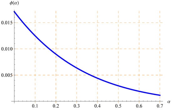
Figure 2.
Plots of in Equation (44) vs. at [km/s], [s], [s] in the range .
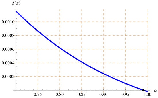
Figure 3.
Plots of in Equation (44) vs. at [km/s], [s], [s] in the range .
7. Conclusions
In this paper, the standard TD formula in the STR is rededuced utilizing an integral approach. Based on such integral approach, the TD is extended in fractional calculus (FC) using the CFD. It is shown that the fractional TD (FTD) is governed by a transcendental equation in terms of the hyperbolic function and the fractional-order , i.e., unlike the explicit standard TD formula in the STR. In addition, it is demonstrated that the present numerical results agree with those of the classical Newtonian mechanics, i.e., , when v is not comparable to c (i.e., ). Moreover, the current numerical results are compared with the experimental ones for the TD of the muon particles . The influence of the arbitrary-order on the variation of the FTD is investigated. The value of at the agreement between the present theoretical results and the corresponding experimental ones is calculated for the TD of the muons particles . The present work may be introduced for the first time to introduce the concept of TD in view of FC. The famous relation between energy E and mass m, known as , may be considered as future directions and potential applications in related fields. Furthermore, the present concept of TD may deserve further extension through other different definitions in FC.
Author Contributions
Conceptualization, E.A.A., M.A. and A.E.; methodology, E.A.A., M.S.A., M.A. and A.E.; software, M.S.A. and A.E.; validation, E.R.E.-Z. and A.E.; formal analysis, M.A., A.E. and H.K.A.-J.; investigation, E.A.A. and M.S.A.; resources, A.E.; writing—original draft, H.K.A.-J.; writing—review & editing, A.E.; visualization, H.K.A.-J.; supervision, E.R.E.-Z.; project administration, E.R.E.-Z.; funding acquisition, E.R.E.-Z. All authors have read and agreed to the published version of the manuscript.
Funding
This study is supported via funding from Prince Sattam bin Abdulaziz University project number (PSAU/2023/R/1444).
Data Availability Statement
Not applicable.
Conflicts of Interest
The authors declare no conflict of interest.
References
- Miller, K.S.; Ross, B. An Introduction to the Fractional Calculus and Fractional Differential Equations; John Wiley & Sons: New York, NY, USA, 1993. [Google Scholar]
- Podlubny, I. Fractional Differential Equations; Academic Press: San Diego, CA, USA, 1999. [Google Scholar]
- Hilfer, R. Applications of Fractional Calculus in Physics; World Scientific Publishing Company: Singapore, 2000. [Google Scholar]
- Narahari Achar, B.N.; Hanneken, J.W.; Enck, T.; Clarke, T. Dynamics of the fractional oscillator. Physica A 2001, 297, 361–367. [Google Scholar] [CrossRef]
- Sebaa, N.; Fellah, Z.E.A.; Lauriks, W.; Depollier, C. Application of fractional calculus to ultrasonic wave propagation in human cancellous bone. Signal Process. 2006, 86, 2668–2677. [Google Scholar] [CrossRef]
- Tarasov, V.E. Fractional Heisenberg equation. Phys. Lett. A 2008, 372, 2984–2988. [Google Scholar] [CrossRef]
- Ding, Y.; Yea, H. A fractional-order differential equation model of HIV infection of CD4+T-cells. Math. Comput. Model. 2009, 50, 386–392. [Google Scholar] [CrossRef]
- Wang, S.; Xu, M.; Li, X. Green’s function of time fractional diffusion equation and its applications in fractional quantum mechanics. Nonlinear Anal. Real World Appl. 2009, 10, 1081–1086. [Google Scholar] [CrossRef]
- Song, L.; Xu, S.; Yang, J. Dynamical models of happiness with fractional order. Commun. Nonlinear Sci. Numer. Simul. 2010, 15, 616–628. [Google Scholar] [CrossRef]
- Gómez-Aguilara, J.F.; Rosales-García, J.J.; Bernal-Alvarado, J.J. Fractional mechanical oscillators. Rev. Mex. Física 2012, 58, 348–352. [Google Scholar]
- Machado, J.T.; Kiryakova, V.; Mainardi, F. Recent history of fractional calculus. Commun. Nonlinear Sci. Numer. Simul. 2011, 16, 1140–1153. [Google Scholar] [CrossRef]
- Garcia, J.J.R.; Calderon, M.G.; Ortiz, J.M.; Baleanu, D. Motion of a particle in a resisting medium using fractional calculus approach. Proc. Rom. Acad. Ser. A 2013, 14, 42–47. [Google Scholar]
- Machado, J.T. A fractional approach to the Fermi-Pasta-Ulam problem. Eur. Phys. J. Spec. Top. 2013, 222, 1795–1803. [Google Scholar] [CrossRef]
- Liaqat, M.I.; Akgül, A.; De la Sen, M.; Bayram, M. Approximate and Exact Solutions in the Sense of Conformable Derivatives of Quantum Mechanics Models Using a Novel Algorithm. Symmetry 2023, 15, 744. [Google Scholar] [CrossRef]
- Ebaid, A. Analysis of projectile motion in view of the fractional calculus. Appl. Math. Model. 2011, 35, 1231–1239. [Google Scholar] [CrossRef]
- Ebaid, A.; El-Zahar, E.R.; Aljohani, A.F.; Salah, B.; Krid, M.; Machado, J.T. Analysis of the two-dimensional fractional projectile motion in view of the experimental data. Nonlinear Dyn. 2019, 97, 1711–1720. [Google Scholar] [CrossRef]
- Ahmad, B.; Batarfi, H.; Nieto, J.J.; Oscar, O.-Z.; Shammakh, W. Projectile motion via Riemann-Liouville calculus. Adv. Differ. Equ. 2015, 63. [Google Scholar] [CrossRef]
- Kumar, D.; Singh, J.; Baleanu, D.; Rathore, S. Analysis of a fractional model of the Ambartsumian equation. Eur. Phys. J. Plus 2018, 133, 133–259. [Google Scholar] [CrossRef]
- Ebaid, A.; Cattani, C.; Al Juhani, A.S.; El-Zahar, E.R. A novel exact solution for the fractional Ambartsumian equation. Adv. Differ. Equ. 2021, 2021, 88. [Google Scholar] [CrossRef]
- El-Zahar, E.R.; Alotaibi, A.M.; Ebaid, A.; Aljohani, A.F.; Gómez Aguilar, J.F. The Riemann-Liouville fractional derivative for Ambartsumian equation. Results Phys. 2020, 19, 103551. [Google Scholar] [CrossRef]
- Ebaid, A.; Masaedeh, B.; El-Zahar, E. A new fractional model for the falling body problem. Chin. Phys. Lett. 2017, 34, 020201. [Google Scholar] [CrossRef]
- Khaled, S.M.; El-Zahar, E.R.; Ebaid, A. Solution of Ambartsumian delay differential equation with conformable derivative. Mathematics 2019, 7, 425. [Google Scholar] [CrossRef]
- Kaur, D.; Agarwal, P.; Rakshit, M.; Chand, M. Fractional Calculus involving (p,q)-Mathieu Type Series. Appl. Math. Nonlinear Sci. 2020, 5, 15–34. [Google Scholar] [CrossRef]
- Iqbal, Z.; Rehman, M.A.-U.; Imran, M.; Ahmed, N.; Fatima, U.; Akgül, A.; Rafiq, M.; Raza, A.; Djuraev, A.A.; Jarad, F. A finite difference scheme to solve a fractional order epidemic model of computer virus. AIMS Math. 2023, 8, 2337–2359. [Google Scholar] [CrossRef]
- Agarwal, P.; Singh, R. Modelling of transmission dynamics of Nipah virus (Niv): A fractional order approach. Phys. A Stat. Mech. Its Appl. 2020, 547, 124243. [Google Scholar] [CrossRef]
- Feng, Y.-Y.; Yang, X.-J.; Liu, J.-G. On overall behavior of Maxwell mechanical model by the combined Caputo fractional derivative. Chin. J. Phys. 2020, 66, 269–276. [Google Scholar] [CrossRef]
- Sweilam, N.H.; Al-Mekhlafi, S.M.; Assiri, T.; Atangana, A. Optimal control for cancer treatment mathematical model using Atangana-Baleanu-Caputo fractional derivative. Adv. Differ. Equ. 2020, 2020, 334. [Google Scholar] [CrossRef]
- Atangana, A.; Qureshi, S. Mathematical Modeling of an Autonomous Nonlinear Dynamical System for Malaria Transmission Using Caputo Derivative. In Fractional Order Analysis: Theory, Methods and Applications; John Wiley & Sons: New York, NY, USA, 2020. [Google Scholar] [CrossRef]
- Fang, J.; Nadeem, M.; Habib, M.; Akgül, A. Numerical Investigation of Nonlinear Shock Wave Equations with Fractional Order in Propagating Disturbance. Symmetry 2022, 14, 1179. [Google Scholar] [CrossRef]
- Aljohani, A.F.; Ebaid, A.; Algehyne, E.A.; Mahrous, Y.M.; Cattani, C.; Al-Jeaid, H.K. The Mittag-Leffler Function for Re-Evaluating the Chlorine Transport Model: Comparative Analysis. Fractal Fract. 2022, 6, 125. [Google Scholar] [CrossRef]
- Ebaid, A.; Al-Jeaid, H.K. The Mittag–Leffler Functions for a Class of First-Order Fractional Initial Value Problems: Dual Solution via Riemann–Liouville Fractional Derivative. Fractal Fract. 2022, 6, 85. [Google Scholar] [CrossRef]
- Einstein, A. Zur Elektrodynamik bewegter Korper. Ann. Der Phys. 1905, 322, 891–921. [Google Scholar] [CrossRef]
- Forshaw, J.R.; Smith, A.G. Dynamics and Relativity; Wiley: Chichester, UK, 2009. [Google Scholar]
- Behroozi, F. A Simple Derivation of Time Dilation and Length Contraction in Special Relativity. Phys. Teach. 2014, 52, 410–412. [Google Scholar] [CrossRef]
- Bailey, J.; Borer, K.; Combley, F.; Drumm, H.; Krienen, F.; Lange, F.; Picasso, E.; Von Ruden, W.; Farley, F.J.M.; Field, J.H.; et al. Measurements of relativistic time dilatation for positive and negative muons in a circular orbit. Nature 1977, 268, 301–305. [Google Scholar] [CrossRef]
Disclaimer/Publisher’s Note: The statements, opinions and data contained in all publications are solely those of the individual author(s) and contributor(s) and not of MDPI and/or the editor(s). MDPI and/or the editor(s) disclaim responsibility for any injury to people or property resulting from any ideas, methods, instructions or products referred to in the content. |
© 2023 by the authors. Licensee MDPI, Basel, Switzerland. This article is an open access article distributed under the terms and conditions of the Creative Commons Attribution (CC BY) license (https://creativecommons.org/licenses/by/4.0/).