Article

Analysis of Evolving Hazard Overflows and Construction of an Alert System in the Chinese Finance Industry Using Statistical Learning Methods

Economics and Management School, Wuhan University, Wuhan 430000, China
Mathematics 2023, 11(15), 3279; https://doi.org/10.3390/math11153279
Submission received: 4 June 2023 / Revised: 11 July 2023 / Accepted: 24 July 2023 / Published: 26 July 2023

Abstract

:
With the global economic situation still uncertain and various businesses interconnected within the finance system, financial hazards exhibit characteristics such as rapid propagation and wide scope. Therefore, it is of great significance to analyze evolving changes and patterns of hazard overflow in the finance industry and construct a financial hazard alert system. We adopt the time-varying parameter vector auto-regressive model to examine the degree and evolving characteristics of financial hazard alerts from an industry perspective and construct financial hazard measurement indicators. To effectively prevent financial hazards and consider the non-linear causal relationship between financial hazards and macroeconomic variables, we utilize the long/short-term memory network model, which can capture temporal features, to construct a financial hazard alert system. Furthermore, we explore whether the inclusion of an online sentiment indicator can enhance the accuracy of financial hazard alerts, aiming to provide policy recommendations on strengthening financial market stability and establishing a hazard alert mechanism under macro-prudential supervision.

1. Introduction

With the continuous improvement of financial innovation and the increasing complexity of transactions, the Chinese financial system has become increasingly interconnected, and financial hazards have gradually exhibited characteristics such as diversification and multi-channel transmission [1]. At the same time, a series of unexpected public events, such as China-US trade friction, the COVID-19 pandemic, and the Ukrainian crisis, have not only intensified uncertainty in the economic industry but also increased the difficulty of hazard prevention and control. Effectively addressing financial hazards remains a major challenge for related regulatory authorities. Therefore, exploring the evolving changes about financial hazard overflows and establishing a hazard alert system can help identify the overall hazard level of the finance industry, develop financial hazard prevention plans, and enhance the ability to guard against hazards [2].
Financial hazard overflow refers to the phenomenon in which hazards originating from financial institutions or markets in one area spread to other related financial institutions or markets, resulting in broader impacts. When a financial institution or market faces hazards and encounters problems, these risks can propagate into other financial institutions, markets, industries, or even countries, leading to a chain reaction effect and triggering systemic hazards. Therefore, one of the important characteristics of financial hazard is hazard overflow, and a considerable amount of research has focused on this area, which can be broadly classified into two categories. The first category involves using indicators such as Conditional Value-at-Risk (CoVaR) and Marginal Expected Shortfall to measure hazard overflow among financial institutions and analyze the mechanisms of financial hazard contagion. However, these methods fail to consider the interdependence between and volatility of financially relevant time-series data [3]. Therefore, some researchers have further employed time-varying generalized the auto-regressive conditional heteroscedasticity model and the rolling window dynamic Copula method to calculate indicators such as CoVaR to study systemic hazard overflows [4]. The second category involves analyzing financial hazard overflow via variance decomposition-based information overflow indicators and examining the evolving changes in hazard overflow via rolling windows [5]. However, in the process of variance decomposition, the contributions of individual factors are combined into a single overall indicator, leading to partial information loss. Therefore, the method’s limitations lie in its potential inability to provide detailed information about hazard overflow or the impact level of specific factors. Additionally, when the evolving changes of hazard overflow are analyzed using rolling windows, the variance decomposition results for each window period are aggregated into a single indicator or value to reflect the hazard overflow within that window period. This aggregation may result in the inaccurate reflection of certain details or specific factors, leading to information loss. The information referred to here includes the contributions of individual financial institutions or markets to overall hazard overflow, the impact level of specific factors, and the hazard overflow within each window period [6]. Therefore, some researchers have used Time-Varying Parameter Vector Auto-Regressive (TVP-VAR) models to construct hazard overflow indicators and analyze their evolving characteristics [7]. Others have employed complex network techniques to study financial hazard overflow, such as examining the evolution of extreme hazard overflow among nine sub-markets in the financial market using weighted networks [8]. Furthermore, Yang et al. [9] have studied financial market contagion relationships among countries along the Belt and Road using the TENET network model.
The term “hazard alert system” refers to the timely issuance of alerting signals derived via monitoring, analysis, and evaluation of various hazard factors in financial markets, enabling financial institutions, government agencies, and investors to take appropriate measures to address potential hazards. The purpose of a hazard alert system is to detect and identify early signs of potential financial crises or systemic hazards so that timely actions can be taken to mitigate the impact of hazards or prevent the occurrence of a crisis [10]. Hazard alert models such as the factor hazard model and stochastic time-varying model were initially developed to target currency crises or international payment crises [11]. However, these models have not provided satisfactory explanations about financial time-series data [12]. With the development of technologies such as artificial intelligence (AI) and big data, an increasing number of computer techniques are being applied in the field of economics [13,14]. Machine learning, in particular, has been widely used in financial forecasting, with some researchers finding that support vector machine (SVM) exhibit high prediction accuracy [15]. Other researchers believe that the artificial neural network (ANN) model yields more accurate prediction results [16]. Traditional machine learning methods have certain limitations in data processing, while deep learning methods can overcome these issues. Specifically, traditional machine learning methods typically rely on manually selected and engineered features and employ shallow models for prediction. In the field of financial forecasting, financial data often exhibits highly complex structures and dynamics, containing numerous nonlinear relationships and random fluctuations. Traditional machine learning methods may struggle to capture these intricate relationships and patterns adequately or require the expertise of domain specialists to select and construct features. In contrast, deep learning methods possess greater data-processing capabilities. By utilizing multi-layer neural network architectures, deep learning can automatically learn higher-level representations of features from raw data and model complex relationships through multiple layers of nonlinear transformations. Deep learning methods are adept at handling data on a large scale and extracting more abstract features, enabling them to better adapt to the complexity and temporal nature of financial data. Therefore, applying deep learning methods to the prediction of financial time-series data is reasonable and effective. For example, in the prediction of stock prices or returns, Long Short-Term Memory (LSTM) models have been shown to outperform traditional machine learning models [17]. To further improve prediction accuracy, Zhang et al. [18,19] used an Average Stochastic Gradient Descent and Weight-Dropped LSTM (AWD-LSTM) model to overcome over-fitting, unstable training data, and other weaknesses, and significant achievements have been made.
By reviewing the studies above and Table 1, it can be observed that currently, research on financial hazard overflow and hazard alert systems have been conducted separately, to the best of my knowledge. Comprehensive research on these topics requires knowledge from multiple domains, including finance, economics, hazard management, and computer science. In addition, it may necessitate collaboration and communication among experts from different fields to conduct integrated research. However, once the study of financial hazard overflow and hazard alert system is combined, it enables hazardous generation, propagation, and monitoring and warning mechanisms to be comprehensively considered, providing a more comprehensive and in-depth understanding. This integrated research can help people better comprehend the nature of financial hazard and explore the interactions between hazard propagation and warning mechanisms. Through comprehensive research, more accurate and comprehensive hazard assessments and decision support can be provided, thereby strengthening financial stability and hazard management capabilities. Indeed, this is precisely the unique aspect of the proposed method. Specifically, this paper selects 30 financial institutions as research samples and uses the Time-Varying Parameter Vector Auto-Regressive (TVP-VAR) model to study the hazard overflow effect in the financial industry and construct financial hazard measurement indicators. It examines the nonlinear relationship between macroeconomic state variables such as returns, volatility, short-term liquidity spreads, and financial hazards. Additionally, the paper incorporates OSIs (Online Sentiment Indicators) into the LSTM model to construct a financial hazard alert system. The overall sketch is shown in Figure 1, and the contributions of this paper are twofold:
(1) First, we use the TVP-VAR model to study evolving hazard overflow effects and directional overflow from the perspective of the financial industry, enriching the theoretical foundation of hazard prevention and control;
(2) Second, we use the LSTM model to verify the alert results of macroeconomic state variables on financial hazards and further investigate whether OSIs can improve alert accuracy, providing reference for global economic hazard prevention and macro-prudential regulation.

2. Materials and Methods

2.1. Analysis of Evolving Hazard Overflows Using TVP-VAR

Jimenez et al. [20] used variance decomposition to study the direction and intensity of financial hazard overflow and employed rolling windows to analyze the evolving effects. In contrast, Adjei [21] utilized TVP-VAR, which does not involve rolling windows analysis. This approach allows for a more flexible and robust capture of potential changes in the underlying structure of the data, thus providing a better characterization of hazard overflow and contagion properties. Our study takes the advantages of both [20,21], specifically, using daily high and low prices to calculate the variance of each institution on a daily basis, and further computing the annualized daily volatility.
σ i t 2 = 0.361 [ ln ( P i t max ) ln ( P i t min ) ] 2
σ ^ i t = 100 365 σ i t 2
in which σ i t 2 represents the estimated daily variance of institution i (i.e., an industry) at day t, P i t max represents the maximum (high) price in institution i at day t, P i t min represents the minimum price of institution i at day t, and σ ^ i t represents the annualized daily volatility of institution i at day t. Due to the relationship between the daily range of prices and the volatility and variance of prices in the financial field, the constant 0.361 is an empirical value used to adjust the calculation results of the daily range variance to better align with market reality. The constant 365 represents the number of trading days in a year, and multiplying by 365 serves to convert the daily variance to an annualized variance. When daily volatility is scaled to an annual scale, it provides a better reflection of the institution’s annual volatility level. Multiplying by 100 is performed to express the volatility as a percentage. Representing volatility as a percentage allows for a more intuitive understanding and comparison of the volatility of different institutions [22].
Furthermore, the TVP-VAR(p) process is established as follows:
{ y t = A t Z t 1 + ε t s . t . ε t | Ω t 1 ~ N ( 0 , Σ t )
{ v e c ( A t ) = v e c ( A t 1 ) + ξ t s . t . ξ t | Ω t 1 ~ N ( 0 , Ξ t )
in which y t represents the column vector of volatility at day t, Z t 1 = ( y t 1 , y t 2 , , y t p ) T   and   A t = ( A 1 t , A 2 t , , A p t ) T represent time-varying coefficients, v e c ( · ) is the vectorized representation, and Σ t and Ξ t represent time-varying variance–covariance matrices. The time-varying coefficients and time-varying variance–covariance matrices are estimated iteratively with the Kalman filter. Due to space limitations, please refer to [23] for more details. The constraints in (3) and (4) are the classical assumptions for the probability distribution of the random error terms in time-series analysis. Specifically, given the information observed up to day t − 1, the distribution of the random variable follows a normal distribution with a mean of 0 and a covariance matrix of Σ t or Ξ t . This assumption is commonly used in statistical inference and modeling methods. In this context, ε t or ξ t and Σ t or Ξ t represent the conditional distribution relationship. ε t represents the random error term in the observation equation, indicating the error in the observed data. On the other hand, ξ t represents the state error term in the state equation, reflecting the variability in parameters or states. Therefore, their distributions are not the same.
With time-varying coefficients and a time-varying covariance matrix, the variance decomposition is calculated [21], transforming the TVP-VAR model into:
{ y t = J T ( M t k 1 Z t k 1 + j = 0 k M t j η t j ) s . t .   M t = ( A t I m ( p 1 ) 0 m ( p 1 ) × m )   η t = ( ε t 0 0 ) T = J ε t J = ( 1 , 0 , , 0 ) T .
Variance decomposition is defined as the proportion of xj in the prediction error variance of H steps forward when variable xi is impacted at time t, in which the contribution of xj to the changes is variable xi. Generalized Forecast Error Variance Decomposition (GFEVD), i.e., matrix dij,t(H), is as follows:
{ d i j , t ( H ) = σ i i , t 1 h = 0 H 1 ( e i T B h , t Σ u , t e j ) 2 h = 0 H 1 ( e i T B h , t Σ u , t B h , t T e i ) . s . t . B h , t = J T M t h J , h = 0 , 1 ,
where σ i i , t 1 represents the i-th element on the diagonal of the matrix. Σ u , t , and Σ u , t represent the time-varying covariance matrix of the disturbance vector ut. ej denotes the unit vector in which the j-th element is 1 and the rest are 0. H represents the forecast horizon, and h represents the lag order of the disturbance vector. To better measure the volatility overflow effect, the variation matrix is normalized, that is:
{ j = 1 m d ˜ i j , t ( H ) = 1 i , j = 1 m d ˜ i j , t ( H ) = m ,
and GFEVD ( d ˜ i j , t ( H ) ) is calculated as:
d ˜ i j , t ( H ) = d i j , t ( H ) j = 1 m d i j , t ( H )
in which d ˜ i j , t reflects the degree of hazard overflow between financial industry i and financial industry j at day t.
Further, the hazardous exposure effect and hazard overflow effect of the i-th industry at day t are defined as the in-degree (from) and out-degree (to), respectively:
S i , t f r o m = j = 1 i j m d ˜ i j , t
S i , t t o = i = 1 i j m d ˜ i j , t .
Finally, the net overflow effect and Financial Hazard Overflow (FHO) indicator of industry i at time t are defined as follows:
N e t i , t = S i , t t o S i , t f r o m
F H O t = i , j = 1 , j i m d ˜ i j , t ( H ) i , j = 1 m d ˜ i j , t ( H ) × 100 = i , j = 1 , j i m d ˜ i j , t ( H ) m × 100
Table 2 presents the hazard overflows among different financial industries at day t.

2.2. Construction of an Hazard Alert System Using LSTM

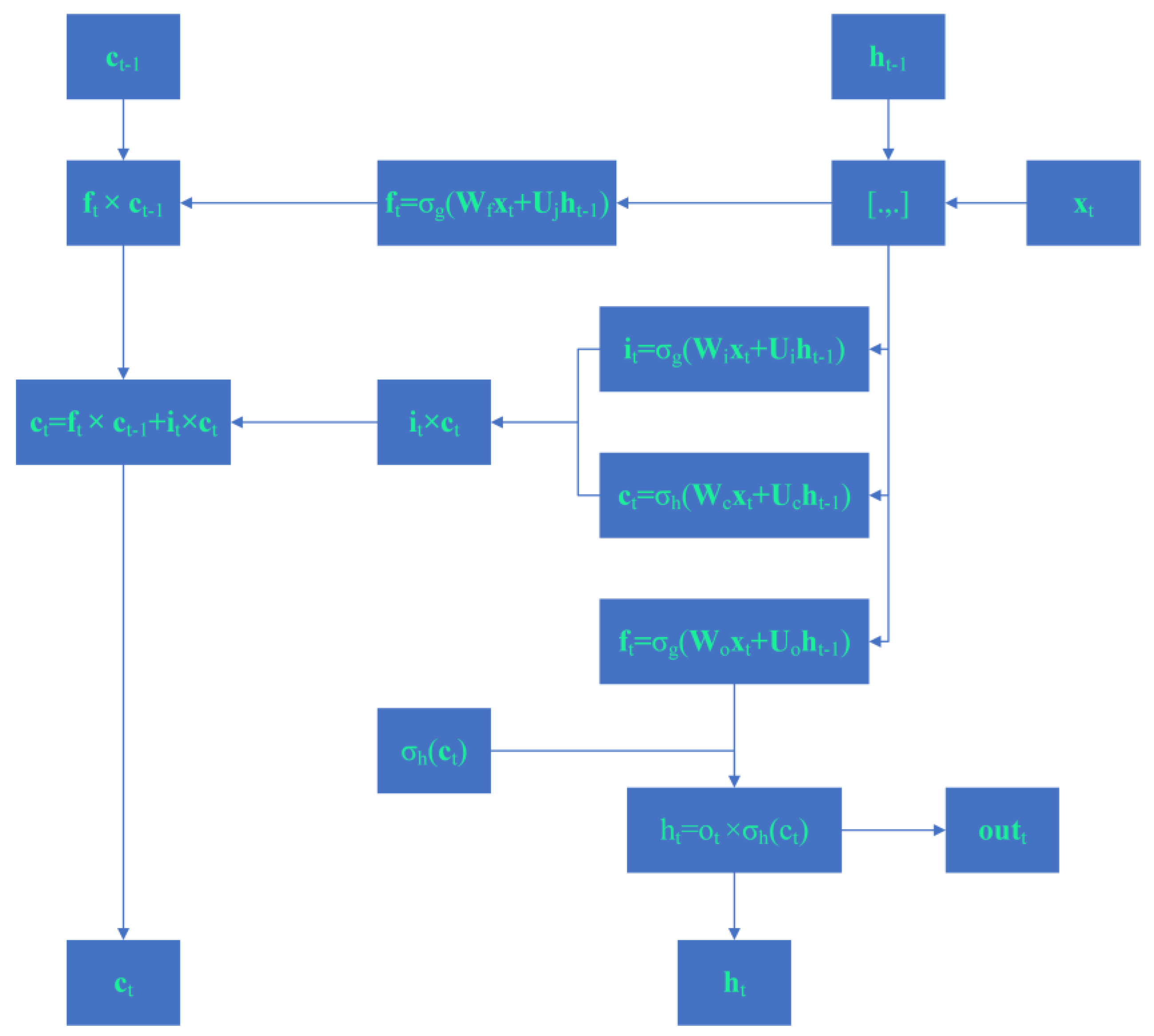
In this paper, the LSTM network is adopted as the alert model. LSTM is a type of recurrent neural network (RNN) that can address issues commonly found in RNNs, such as gradient explosion or vanishing gradient. It is suitable for processing and predicting time-series data. Figure 2 illustrates the recurrent unit structure of LSTM. The matrices W and U represent the weights for input connections and recurrent connections, respectively. These weights include bias terms, and the subscripts of the weights denote the input gate (i), output gate (o), forget gate (f), and memory cell (c). σ denotes the activation function; × represents the Hadamard product. xt is the vector input to the LSTM unit, ft is the vector after the activation of the forget gate, it is the vector after the activation of the input gate, ot is the vector after the activation of the output gate, ht is the hidden state vector, ht−1 represents the hidden state of the previous time step, c ˜ t is the vector after the activation of the cell input, ct is the cell state vector, ct−1 represents the cell state of the previous time step, xt represents the input data, xt−1 represents the input data of the previous time step, and xt represents the output data. In this paper, LSTM is utilized to learn about historical financial alert indicators and attempt to predict future alert indicators. Please refer to Section 3.2.1 for more details.
The working mechanism of LSTM is as follows: The forget gate considers the information to be discarded from the cell, observing ht−1 and xt−1, and performs the operation ft = σg(Wfxt + Ujht−1). At this point, each cell state ct−1 outputs a value between 0 and 1, with 1 representing complete retention and 0 representing complete discard. The input gate considers preserving and updating information from the cell state, where it = σg(Wixt + Uiht−1) determines which values need to be updated. c ˜ t = σ h ( W c x t + U c h t 1 ) generates a candidate vector that can be added to the cell for combination. The calculation i t × c ˜ t is performed to update the old state. The output gate considers outputting information based on the filtered cell state σh(ct), resulting in a value between −1 and 1. The corresponding output ht is then calculated by combining it with the output gate state.
In order to assess the predictive accuracy of the LSTM network model, Mean Absolute Error (MAE) and Mean Square Error (MSE) have been chosen as evaluation metrics. The smaller the values of these two metrics, the closer the model’s predictions are to ground truths, indicating a better predictive performance of the model. The specific formulas for calculating these metrics are as follows:
M A E = 1 N i = 1 N | g ˜ i p i |
M S E = 1 N i = 1 N ( g ˜ i p i ) 2
where g and p represent the ground truth and model prediction value respectively, and N is the sample size.

3. Research and Analysis

3.1. Analysis about Evolving Hazard Overflows

3.1.1. Data Source and Analysis

The banking industry is the mainstay of the financial system and also the primary focus of hazard monitoring and macroprudential supervision. In addition, the insurance industry, securities industry, and diversified financial industry play important roles in the financial system. To study hazard overflow, we selected financial institutions listed on the Shanghai and Shenzhen stock exchanges before 1 January 2010 as samples representing the banking, insurance, securities, and diversified financial sub-industries. After excluding financial institutions with missing data, the final sample included 14 banks, 3 insurance companies, 8 securities firms, and 5 diversified financial firms, and Table 3 provides the list and identification numbers of the selected institutions. If monthly or quarterly data had been selected, it would not have effectively tracked the changes in the financial market and could have led to significant research errors. Therefore, we calculated volatility using the daily high and low prices of each financial institution, covering the period from 1 January 2010, to 31 December 2022. All data are sourced from the China Stock Market Accounting Research [24] and Wind databases [25].
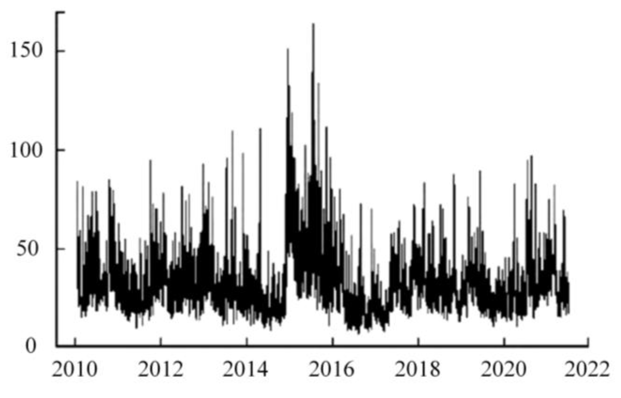
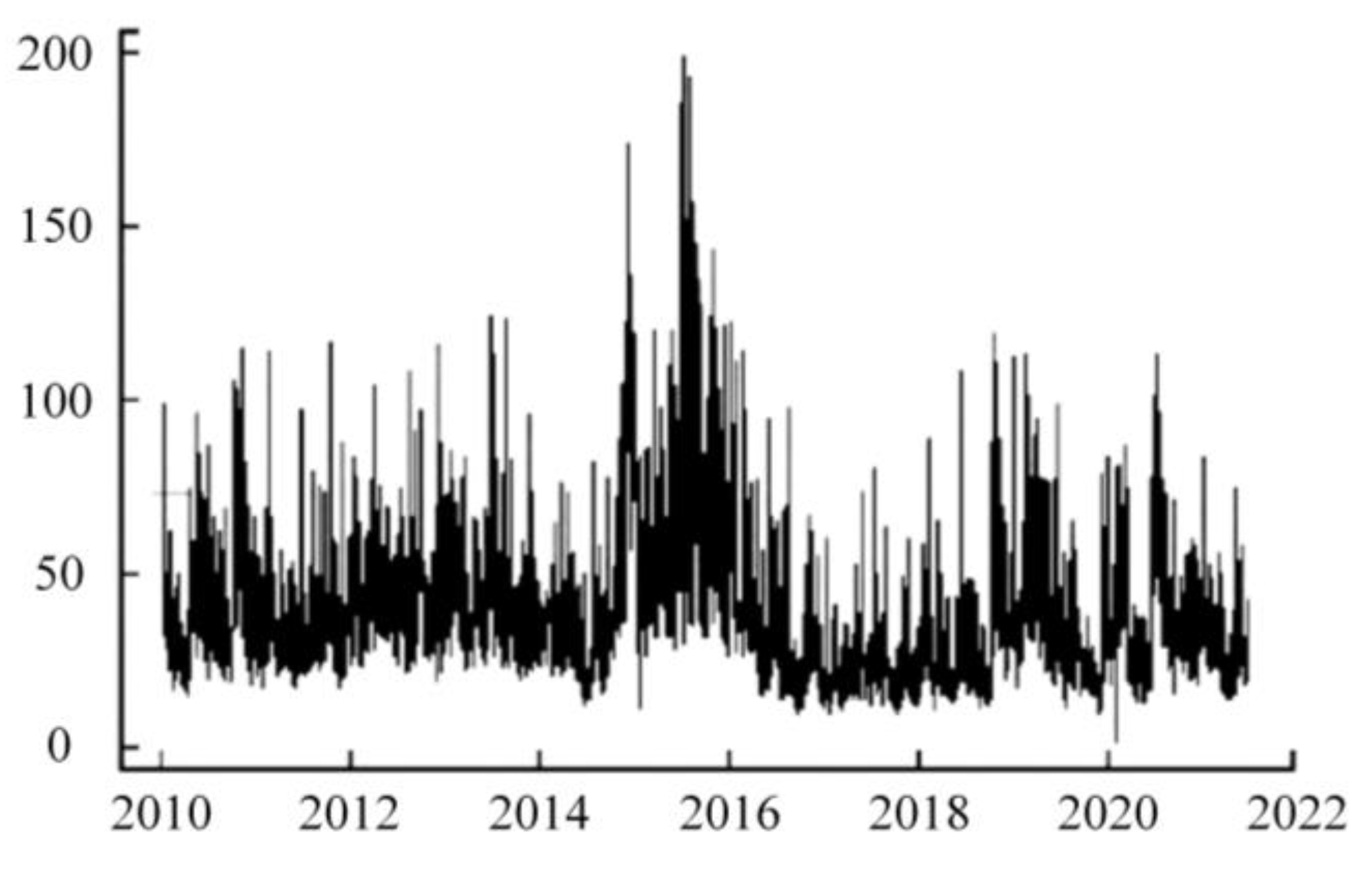
Figure 3, Figure 4, Figure 5 and Figure 6 show the time-series plots of average volatility for the four industries.
Overall, the volatility patterns of the four industries are similar. The most significant volatility occurred in 2015, reaching its peak. This could be attributed to the deleveraging policy implemented by regulatory authorities in the second half of 2015, which caused market panic and a massive sell-off of stocks by investors, leading to extreme turbulence in the stock market. Volatility also occurred during the liquidity crunch in 2013, the COVID-19 crisis in 2020, and the Ukrainian crisis in 2022, indicating that the constructed volatility measure in this paper effectively captures the changes in industry hazard.
Table 4 provides statistical descriptions of the volatility in the four industries.
As shown in Table 4, the banking industry has the lowest mean volatility of 26.09 and the lowest standard deviation of 15.60, indicating the smallest fluctuation in volatility among the four industries. In contrast, the securities industry exhibits the highest level of volatility, suggesting that the banking industry has relatively stable volatility, while the securities industry experiences greater volatility stability issues.

3.1.2. Analysis of Evolving Hazard Overflows

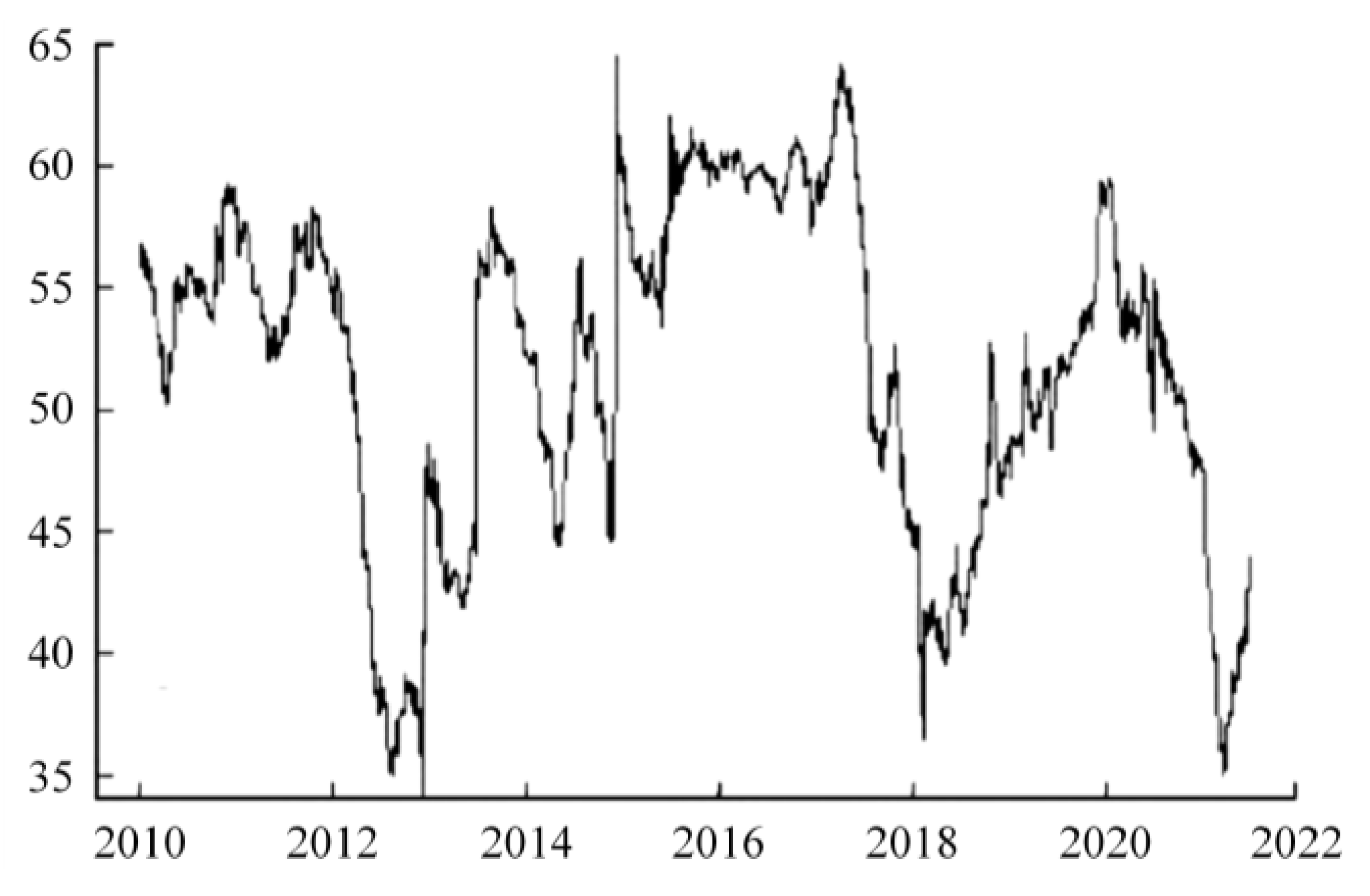
In this section, the TVP-VAR model is used to analyze the evolving hazard overflows in four financial industries in China. Specifically, this section discusses hazard overflows from overall to specific. Figure 7 shows the time-series plot of hazard overflows in the financial system.
Figure 7 shows that the range of the financial hazard overflow indicator is between 35% and 65%. Around 2013, 2015, and 2020, the financial hazard overflow indicator increased significantly, indicating that events such as the liquidity crunch, stock market crash, COVID-19 pandemic, and Ukrainian crisis have impacted the financial industry, intensifying financial hazards. This also confirms that the financial hazard overflow indicator calculated using the proposed TVP-VAR model can serve as a measure of financial hazard, effectively capturing the time-varying characteristics of financial hazards. Specifically, from 2010 to 2012, the financial hazard overflow indicator remained at the high level of 50–60%, possibly influenced by events such as the European debt crisis. After 2012, there was a noticeable downward trend. Following the impact of the liquidity crunch in 2013, the financial hazard overflow indicator increased from around 42% to 58% and remained high until 2014, when it started to decline. In the second half of 2015, the deleveraging policy implemented by regulators led to significant turbulence in the stock market, causing a sharp increase in financial hazard. During this period, the financial hazard overflow indicator reached a peak of 65% and remained elevated for a considerable period. In 2018, the overflow indicator increased due to events such as China–US trade friction. Additionally, in early 2020, the outbreak of the COVID-19 pandemic and its rapid global spread, as well as the crisis in Ukraine in 2022, changed investors’ expectations and hazard preferences, leading to a strong adjustment in global stock markets and an increase in financial hazard. This resulted in the overflow indicator reaching a peak of 60% once again.
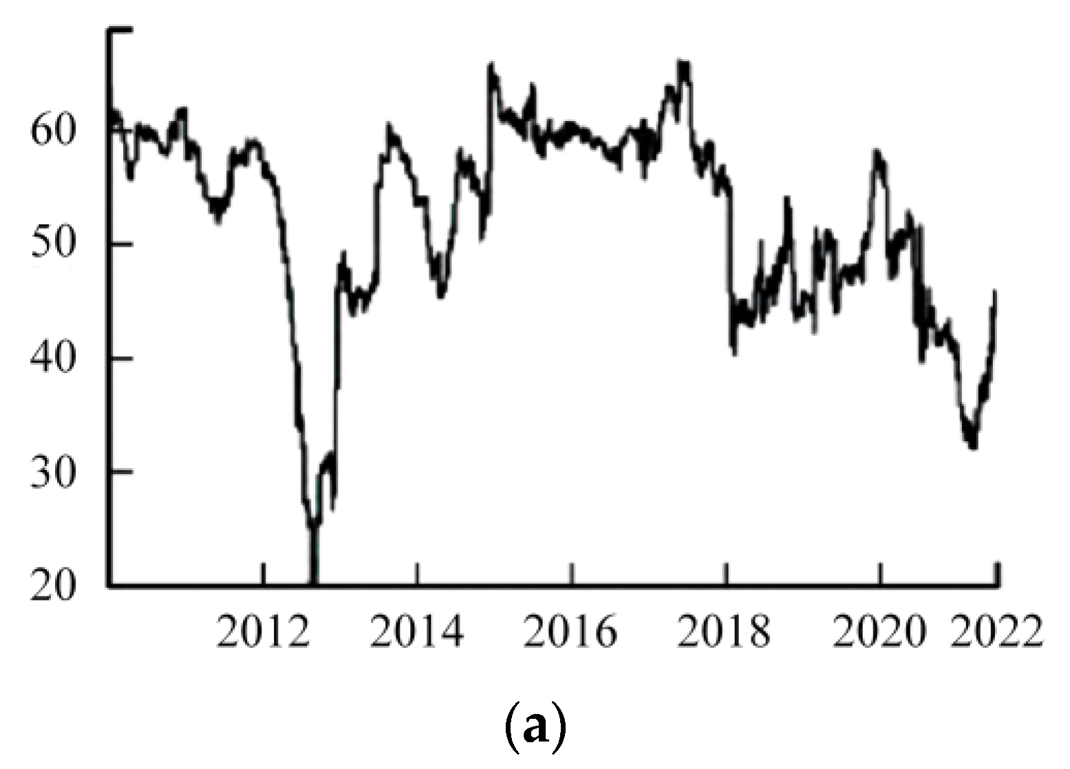
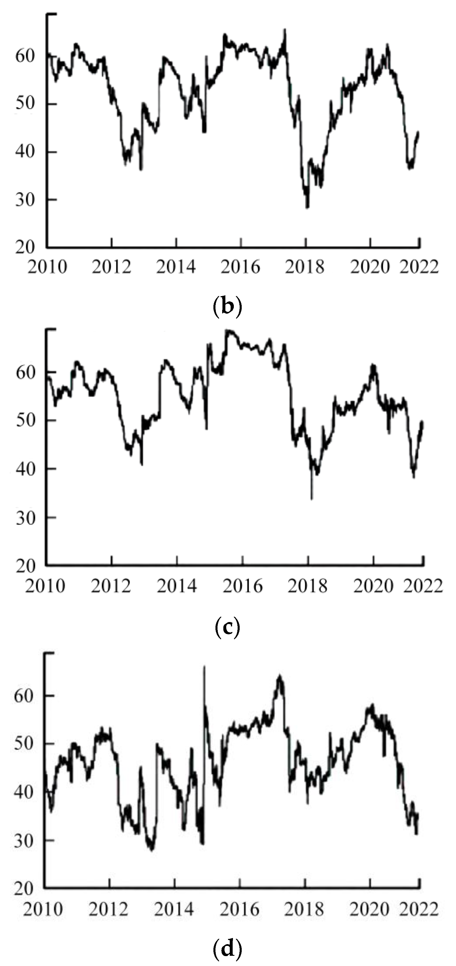
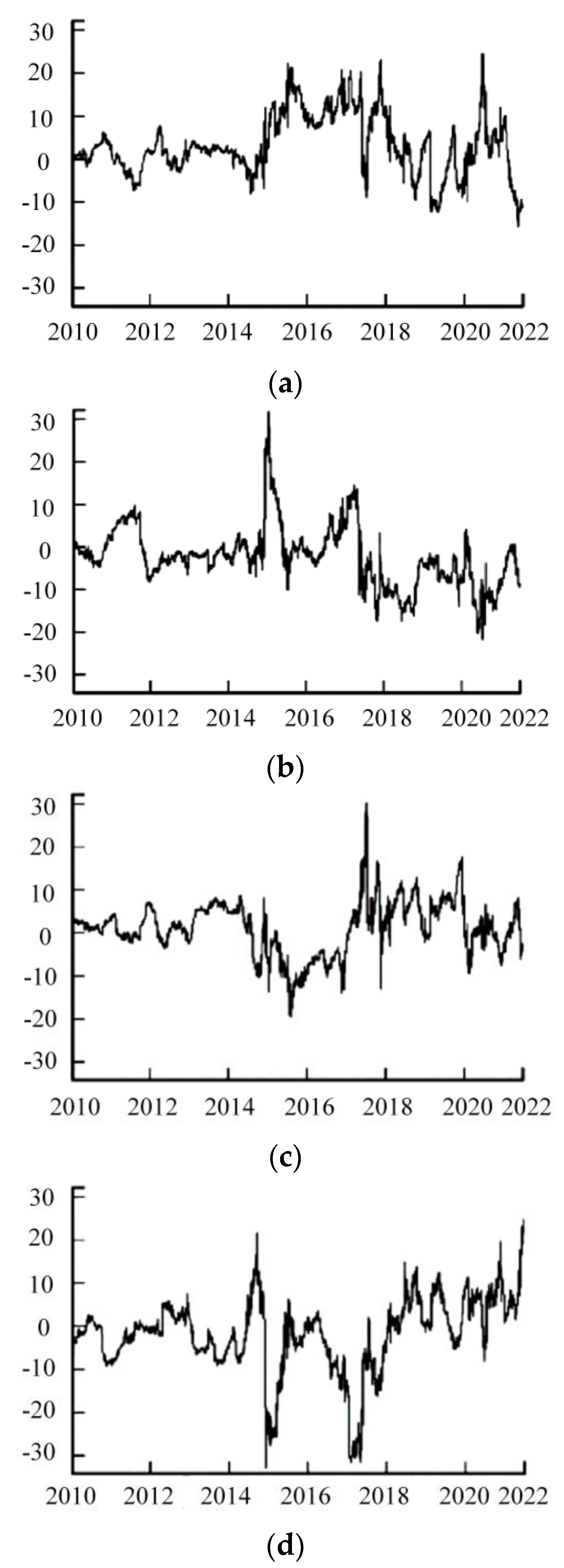
Figure 8a–d analyze the hazard exposures, i.e., the in-degree, of each financial industry and its evolving characteristics.
It can be observed that the in-degree of the four industries shows a similar trend to the financial hazard overflow indicator, indicating that external shocks to the financial system lead to increased hazard exposure in each industry, thereby exacerbating overall financial hazard. Currently, the in-degree of each industry is generally declining, indicating a decrease in the hazards faced by the financial industries in recent years.
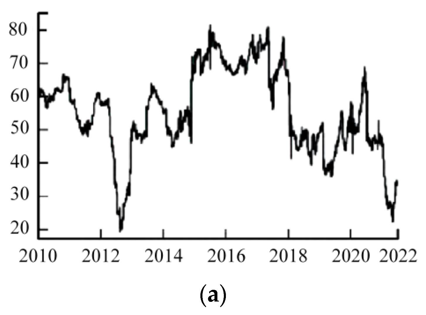
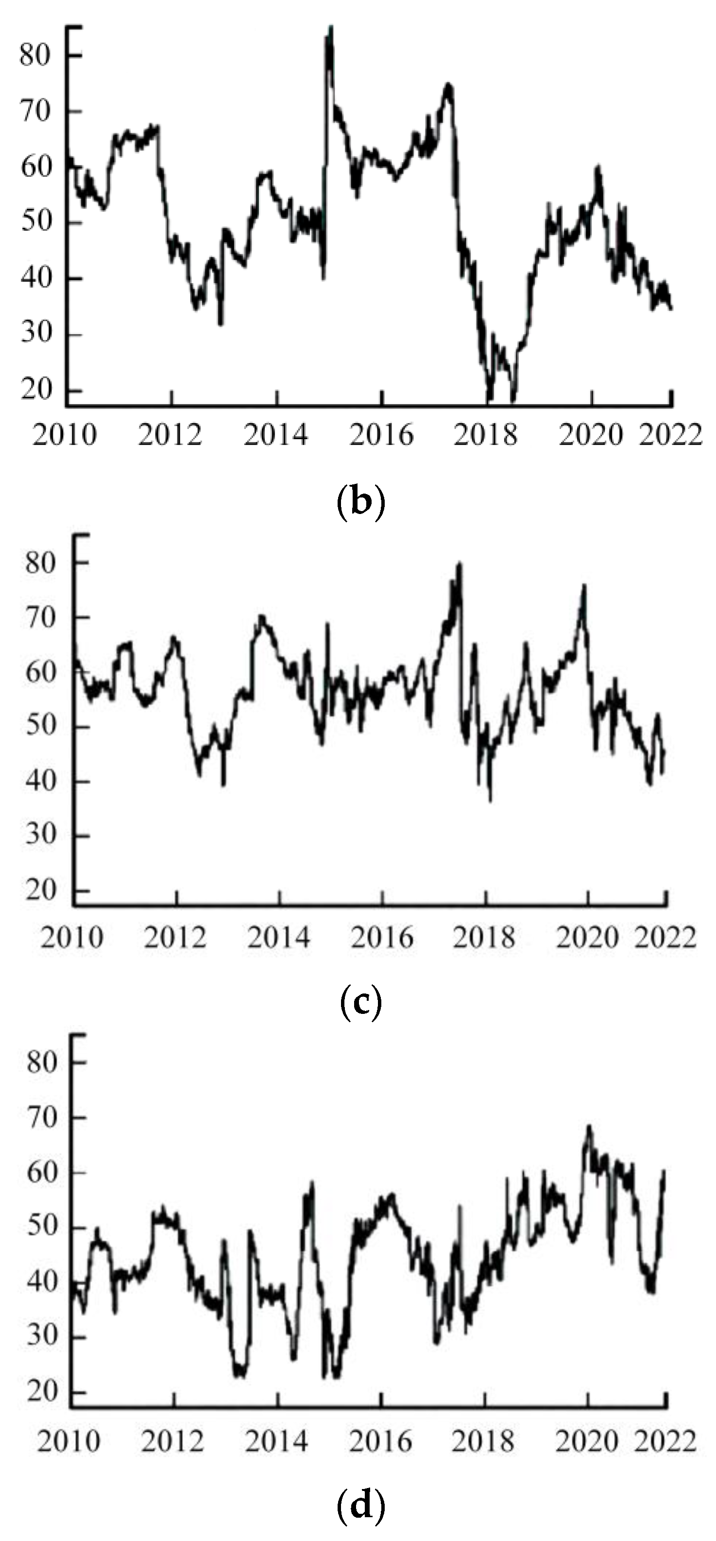
Figure 9a–d depict the hazard overflow, i.e., the out-degree, of each financial industry.
From Figure 9, it can be seen that the out-degree of the four industries shows an upward trend around significant crisis events in 2013, 2015, and 2020, indicating that crisis events intensify the hazard overflow of the financial industries, making each industry a potential carrier of hazard transmission. It is noteworthy that, during crisis events, hazard overflow in the banking industry is the highest, further proving that as the mainstay of the financial system, the banking industry and its related monetary policies and regulatory channels serve as the primary means of macroeconomic regulation and control of other industries [12].
Comparative analysis of the in-degree and out-degree of the financial industries reveals an asymmetry in hazard exposure and hazard overflow. The in-degree and out-degree of the banking and insurance industries are at relatively high levels, while the in-degree of the securities and diversified financial industries is generally higher than the out-degree. During financial system shocks, the in-degree and out-degree of the banking and insurance industries increase. Given that the banking industry is the foundation of the financial system and the insurance industry provides hazard protection to the financial system, these two industries are relatively stable. However, more attention should be given and efforts should be made to strengthen the hazard situation and hazard resistance capabilities of the securities and diversified financial industries.
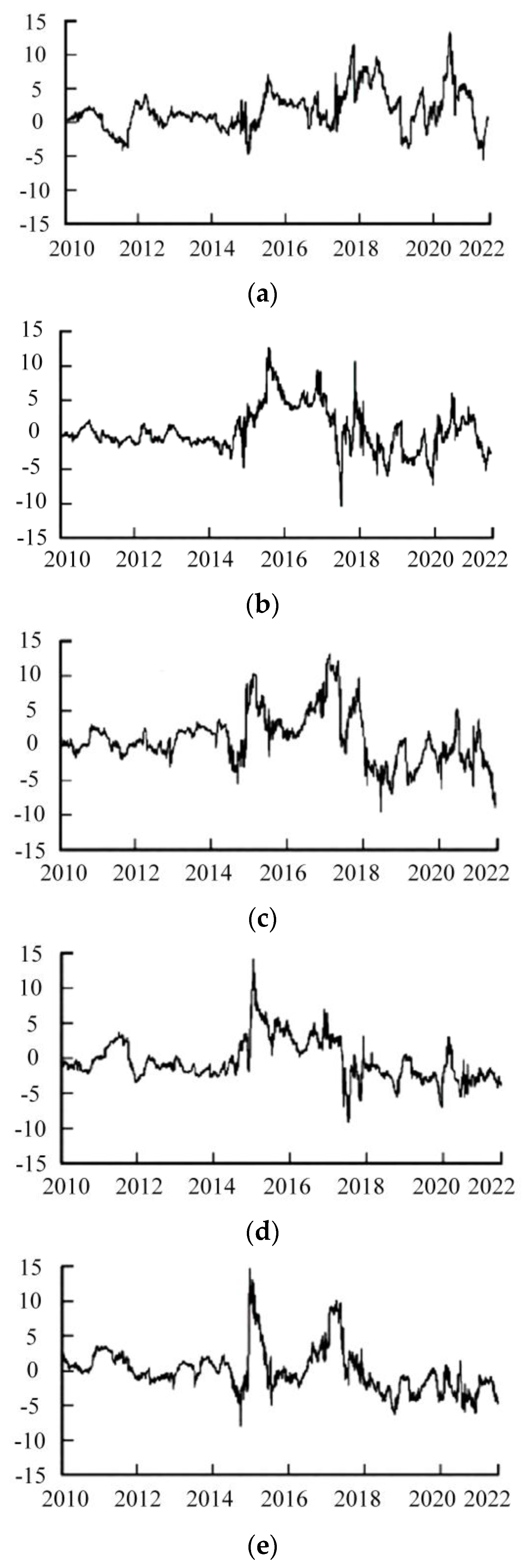
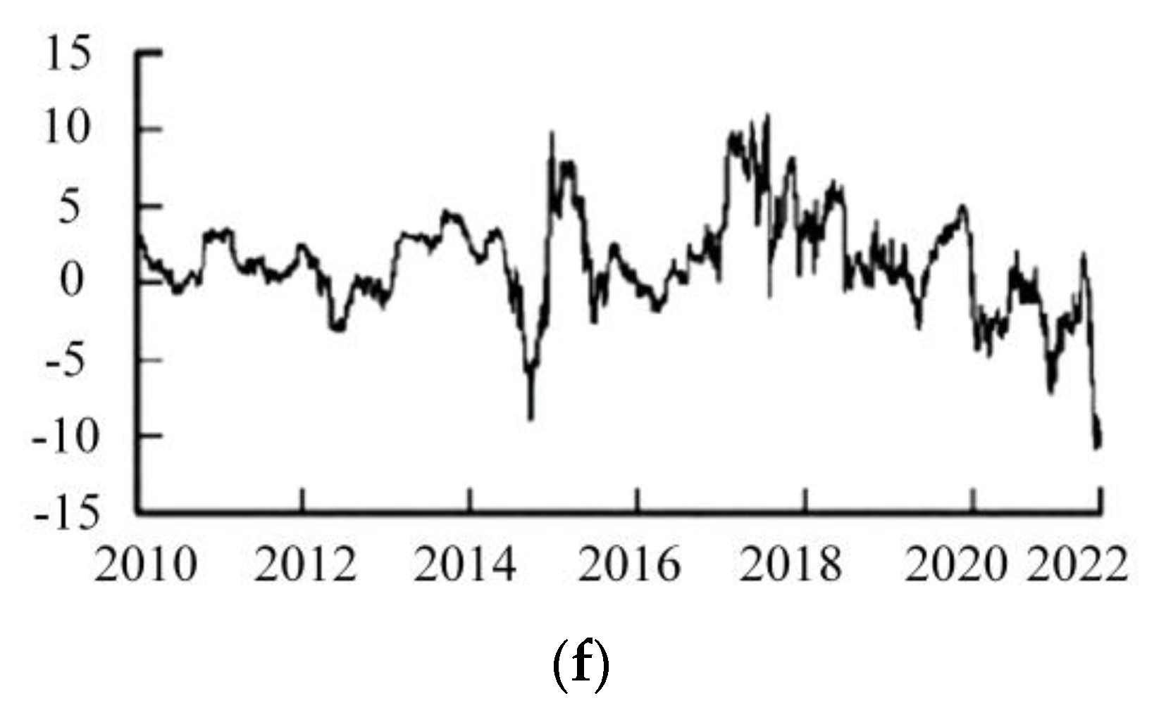
This section further examines hazard transmission direction in the financial industry by analyzing net overflows. Figure 10a,b depict the net overflows within individual financial industries, while Figure 11a–f illustrate the net overflows between pairs of industries. It can be observed that each industry exhibits distinct time-varying characteristics in terms of net overflows, and the net overflow patterns between any two industries also vary, indicating heterogeneity in the net overflows of each industry, which can be attributed to differences in asset size, business type, and regulatory authorities of each industry.
In Figure 10a,b, the banking industry shows mostly positive net overflows, indicating that in most cases, the hazard overflow in the banking industry exceeds the hazard it absorbs. During major crisis events such as the liquidity crunch, stock market crash, COVID-19 pandemic, and Ukrainian crisis, the net overflows in the banking industry increase significantly. The insurance industry experiences the highest net overflow during stock market crashes, while during the COVID-19 pandemic and the Ukrainian crisis, it primarily absorbs hazards. The securities and diversified financial industries act as hazard absorbers during both events.
In Figure 11a–f, there are both overflows and exposures to hazard between pairs of industries, indicating asymmetry and interconnectivity among the financial industries, resulting in complex hazard transmission. During crisis events, the net overflows between pairs of industries increase to varying degrees, indicating enhanced interdependence among the industries. Specifically, among the banking and insurance industries, the banking industry predominantly spills hazards over, while the insurance industry primarily absorbs hazards. Similarly, among the banking and securities industries, and the banking and diversified financial industries, the banking industry mostly spills hazards over, while the securities and diversified financial industries show minimal overflow to the banking industry. This is mainly due to the banking industry’s role as the foundation of financial market and its crucial role in maintaining financial stability. Among the insurance and securities industries, the insurance industry initially spills hazards over in 2015 but later absorbs hazards. The same pattern is observed in the insurance and diversified financial industries, as the insurance industry provides insurance services to financial institutions in other industries, leading to a certain degree of interconnection. In the securities and diversified financial industries, the securities industry primarily spills hazards over, while the diversified financial industry absorbs hazards.
The above analysis demonstrates that the financial hazard overflow indicator calculated using the TVP-VAR model effectively captures the time-varying characteristics and of financial hazards, reveals the inter-dependence among financial industries, and identifies the features and patterns of hazard overflows between industries. In addition, it can be observed that there is an asymmetry in hazard overflow among industries. External shocks enhance the interconnectedness among financial industries, leading to a significant increase in financial hazard overflow indicators. The banking industry exhibits a predominantly positive overflow, and there is an increasing trend during the shock period, indicating the significant role of banks as hazard control entities.

3.2. Analysis of Hazard Alert

3.2.1. Construction of Financial Hazard Alert Indexes and Experiment Settings

Drawing on the research of [1], we selected macro-state variables such as the logarithmic return and volatility of the Shanghai Composite Index and the short-term liquidity spread as alert indicators. As financial hazard also influences its own alert, we included financial hazard in the indicators. The frequency of the alert variables in this paper is daily, so monthly, quarterly, and annual data are not considered. Table 5 shows the final construction of the alert indexes.
We used the LSTM model to construct the alert system for financial hazard. Parameter adjustments were made based on the change in the loss function, and the data set was divided into a 3:1 ratio for training and testing. For the specific structure and parameters, please refer to Table 6.

3.2.2. Construction of the Hazard Alert System

Deep learning can better explore the nonlinear relationships between data and improve prediction accuracy. To verify the effectiveness of the proposed early-warning model, it is necessary to first examine whether macroeconomic variables such as the LR, VO, and SLS can serve as alert indicators for financial hazard. Traditional Granger causal tests can be used to measure the linear causal relationships between variables and determine if a variable can improve the predictive power for other variables. However, most financial time series exhibit nonlinear dynamic patterns, and the selected deep learning model in this paper is a nonlinear alert model. Therefore, non-linear Granger causal tests are adopted to examine the nonlinear relationships between the selected macroeconomic variables and financial hazard, as well as their predictive ability for financial hazard.
Before conducting non-linear Granger causal tests, it is first necessary to examine the existence of nonlinear dynamic relationships between the variables. Thus, following [21], the VAR model is used to filter the linear relationships between variables, with FHO chosen as the dependent variable for regression. The residual sequences are then tested using the BDS (Box Dimension) and RESET (Regression Error Specification Test) methods, with results of 10.822 and 8.017, respectively; both are significant at the 1% level, indicating the presence of nonlinear relationships among the variables. Furthermore, the non-parametric method proposed by [26] is employed for non-linear Granger causal tests. Table 7 shows the test results.
Table 7 clearly indicates the existence of nonlinear relationships between the selected macroeconomic variables and FHO. These variables can serve as alert indicators for FHO, and selecting nonlinear models for financial hazard alert research is justified.
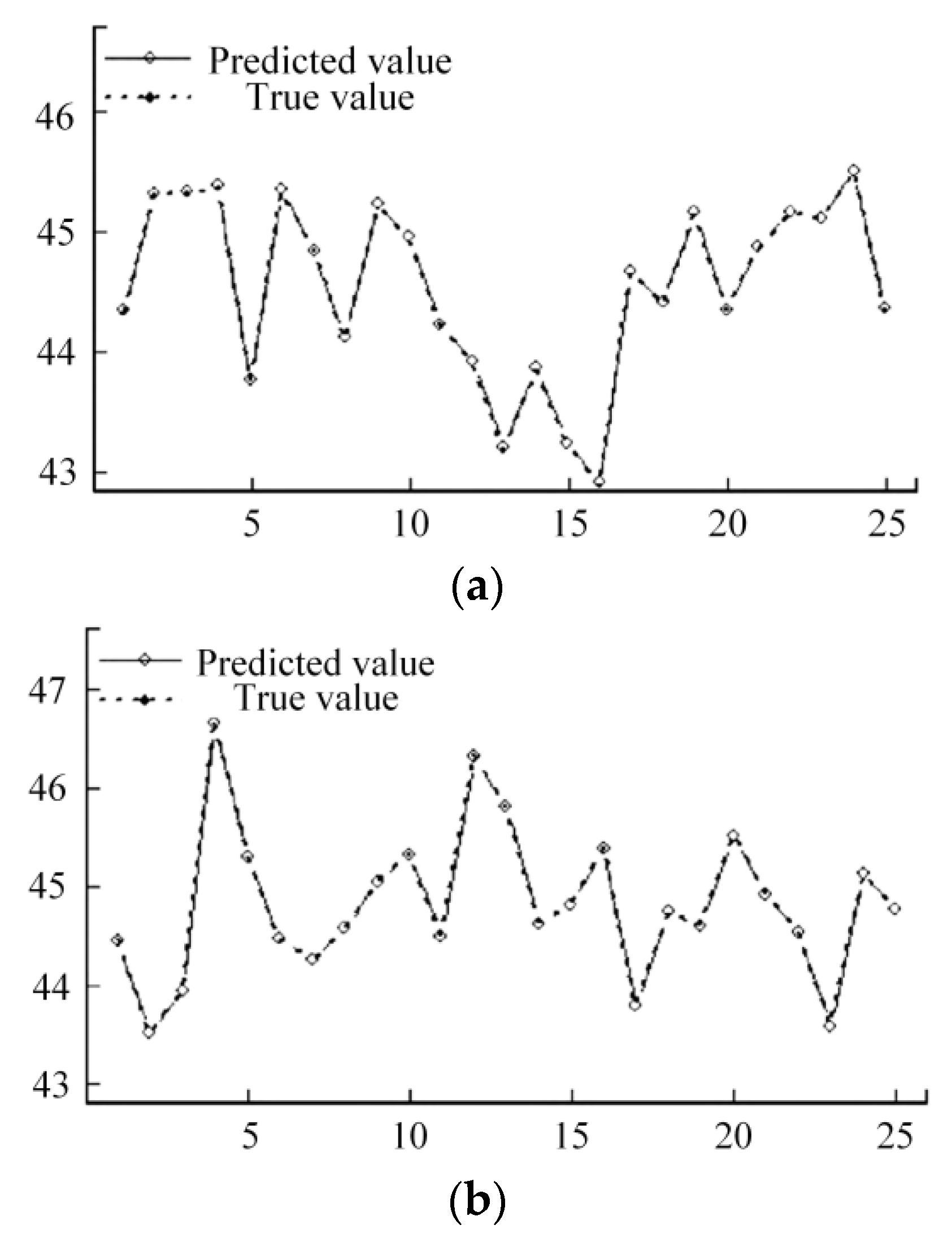
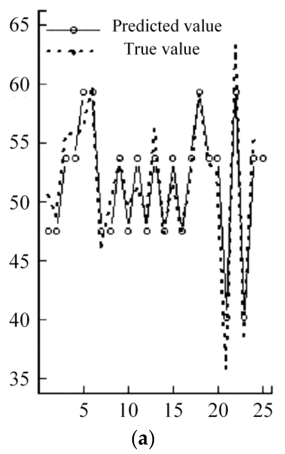
Figure 12a,b and Table 8 show the learning results and errors of the LSTM model for the training and testing sets, respectively. The training set is used to establish the model and learn its own parameters, while the testing set evaluates the generalization ability of the model. As seen in Figure 12, both the training and testing show good performance. Combined with the results in Table 8, the learning error on the testing set is generally small, indicating that the LSTM model constructed in this paper has good generalizability. It also suggests that the selected macroeconomic indexes can serve as effective early warning indexes for financial hazards.
To fully demonstrate the effectiveness of the proposed alert model, artificial neural network (ANN), support vector machine (SVM), random forest (RF), and decision tree (DT) are also chosen for training. Due to the large amount of data, Figure 13, Figure 14, Figure 15 and Figure 16 show the partial training results of each model for clear comparison.
From Figure 13, Figure 14, Figure 15 and Figure 16, it can be observed that the training and testing results of the DT are not ideal. The SVM and ANN models perform better, but visually, the learning results of the RT are comparable to the proposed LSTM model. Therefore, it is necessary to further calculate the learning errors of each model.
Table 9 provides the learning errors of the four models mentioned above.
When Table 8 and Table 9 are combined, it can be seen that the DT model has the largest learning errors in both the training and testing sets, indicating the least desirable training results and the poorest generalization ability. Compared to other models such as BP, SVM, and DT, the RF model shows relatively better learning results. However, when comparing the RF model with the LSTM model, both in terms of MAE and MSE, the LSTM model has the smallest errors. Additionally, the LSTM model demonstrates good predictive ability and generalizability. Therefore, the proposed LSTM model outperforms other models in effectively extracting information between variables and establishing a highly accurate alert model.

3.2.3. Further Analysis—Research on Financial Hazard Alert Incorporating OSI

The strong correlation between online sentiment and financial markets has been widely recognized. Lv et al. [27] indicates that investor sentiment is an important factor affecting stock market stability. Investor attention and sentiment changes can lead to stock volatility and impact systemic hazard. Therefore, incorporating online sentiment into the research on financial hazard alert is of significant importance. Currently, there is no unified standard for constructing OSIs among scholars. The methods can be broadly categorized into three types: obtaining OSIs via market surveys to capture investor opinions, using principal component analysis (PCA) to measure OSIs, and constructing OSIs via text-mining techniques [28,29]. In the era of big data and the internet, online financial media platforms such as stock forums and Bloomberg News provide investors with professional communication platforms. Analyzing relevant text information can better reflect OSIs.
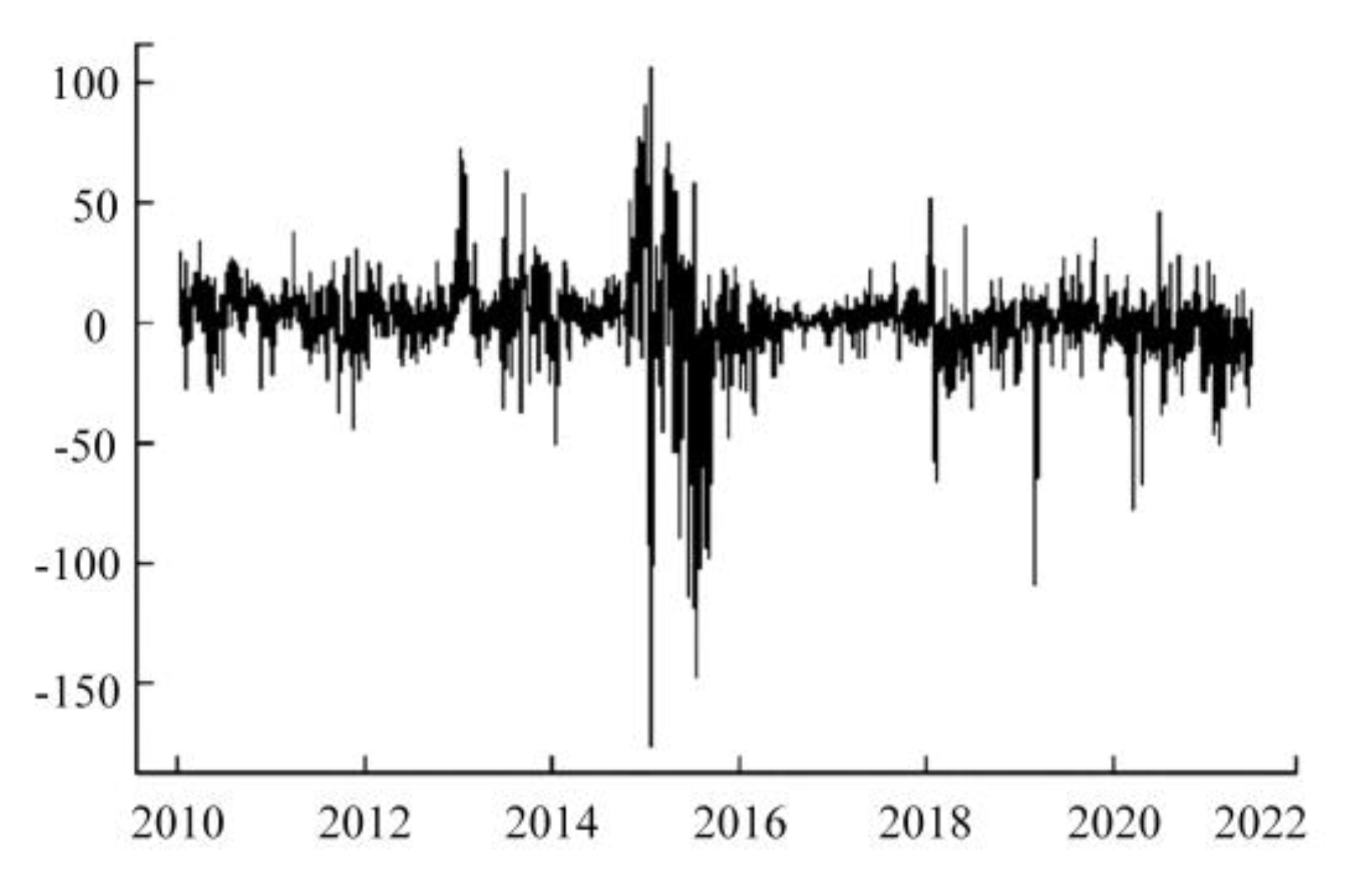
In this paper, we select the individual stock discussion area of 30 listed companies on the East Money website as the source of text information. We use Python to collect comment data from 1 January 2010 to 31 December 2022. The data include post titles, click-through rates, reply counts, usernames, posting time, and post content. After data cleansing, we utilize the Jieba word segmentation library to perform text segmentation and construct an OSI. Figure 17 shows the changes in online sentiment during the sample period.
From Figure 17, we can observe that the overall range of the OSI is [−200, 150], with most fluctuations occurring within the range of [−50, 50] around the scale line. Three periods with significant fluctuations are observed in 2013, 2015, and around 2020, which coincide with significant stock market volatility. Therefore, constructing the OSI in this paper can reasonably reflect changes in investor sentiment.
In the research on alert models incorporating OSIs, it is necessary to examine the predictive ability of the newly incorporated alert indicators for financial hazard. Therefore, based on the selected macro-variables, the OSI is included in the formation of a novel alert indicator system. Nonlinear tests are conducted on the proposed system with a BDS test statistic of 10.789 *** and a RESET test statistic of 7.473 ***. This indicates the existence of nonlinear relationships among the new indexes. Further non-linear Granger causal tests are performed to examine whether the proposed system has predictive power regarding financial hazard. The results indicate the presence of nonlinear causal relationships between the OSI-based alert indicators and financial hazard, thus confirming their potential as alert indicators in the financial hazard alert system.
In addition, we also utilize the LSTM model that has been established in this paper, along with other comparative models, to train with the newly OSI as input and financial hazard as output. Due to limited space, Table 10 only shows the learning errors of different models. MAEa and MSEa represent the learning errors of the alert indexes without the OSI, while MAEb and MSEb represent the learning errors with the inclusion of the OSI.
Through comparison, it is found that among various models, the proposed LSTM model has the smallest learning error, indicating its ability to improve prediction accuracy. Except in the DT model, incorporating the OSI enhances the training accuracy and generalizability of the models. This confirms that the OSI can serve as a financial hazard alert indicator and provide valuable insights for policymakers in formulating hazard policies.

4. Conclusions

In this paper, we conducted an analysis of evolving hazard overflows in the financial industry using statistical learning methods and constructed a financial hazard alert system. Based on our research, the following conclusions can be drawn. Firstly, the study of financial hazard overflow indicates that the overflow indicator calculated using the Time-Varying Parameter Vector Auto-Regressive model can effectively capture changes in financial hazard. Hazard overflow between industries exhibits asymmetry, where external shocks enhance the interconnectivity among the financial industries, leading to a significant increase in the financial hazard overflow indicator. The net overflow in the banking industry is mostly positive and tends to increase during shocks, indicating the significant role of banks as the main entities in hazard control. Secondly, the non-linear Granger causal test demonstrates that there is a non-linear relationship between the selected macroeconomic state variables and financial hazard. These variables can serve as alert indicators of financial hazard. The Long Short-Term Memory model, which can effectively capture and explore the non-linear relationships among data, is capable of incorporating these variables into the financial hazard alert system. Lastly, the constructed online sentiment indicator reflects changes in investor sentiment. The online sentiment indicator exhibits non-linear predictive capability for financial hazard. By incorporating this into the financial hazard alert system, alert accuracy can be further enhanced. This suggests a close correlation between online sentiment and financial hazard. Therefore, it is important to consider the impact of online sentiment and take accurate and effective measures to prevent the contagion and spread of financial hazards.

5. Managerial Insights

The research on financial hazard overflow and alert has significant practical implications in the following aspects:
(1) Hazard management: Understanding the overflow and transmission mechanisms of financial hazards helps institutions and governments take timely measures to address potential hazards. With a hazard alert system, potential signs of financial crises or systemic hazards can be detected in advance, enabling appropriate actions to mitigate hazard impact or prevent crises.
(2) Financial stability: Understanding the overflow effects of financial hazards helps assess interconnected hazards in the financial system and take measures to maintain financial stability. By studying financial hazard overflow, a better understanding of interdependencies among financial institutions and markets can be achieved, thereby enhancing the resilience and stability of the financial system.
(3) Cross-border hazard management: Research on financial hazard overflow aids in identifying hazard transmission channels in cross-border financial systems, facilitating international cooperation and cross-border regulation to collectively address global financial hazards. Understanding financial hazard overflow promotes international information sharing, establishment of cooperation mechanisms, and formulation of cross-border hazard management policies.
(4) Investment decision-making: Studies on hazard alert and overflow provide crucial reference information for investors. Understanding the degree and influencing factors of hazard overflow helps investors better evaluate portfolio hazards, optimize asset allocation, and reduce investment hazard.

Funding

This research received no external funding.

Data Availability Statement

No new data were created or analyzed in this study. Data sharing is not applicable to this article.

Conflicts of Interest

The author declares no conflict of interest.

References

  1. López-Espinosa, G.; Moreno, A.; Rubia, A.; Valderrama, L. Short-term wholesale funding and systemic risk: A global CoVaR approach. J. Bank. Financ. 2012, 36, 3150–3162. [Google Scholar] [CrossRef] [Green Version]
  2. Derbali, A.; Hallara, S. Systemic risk of European financial institutions: Estimation and ranking by the Marginal Expected Shortfall. Res. Int. Bus. Financ. 2016, 37, 113–134. [Google Scholar] [CrossRef] [Green Version]
  3. Engle, R. Systemic risk 10 years later. Annu. Rev. Financ. Econ. 2018, 10, 125–152. [Google Scholar] [CrossRef]
  4. Wu, F.; Zhang, Z.; Zhang, D.; Ji, Q. Identifying systemically important financial institutions in China: New evidence from a dynamic copula-CoVaR approach. Ann. Oper. Res. 2021, 1–35. [Google Scholar] [CrossRef]
  5. Cao, J.; Lei, L.; Zhang, R.; Lei, Q. Risk of spillovers between the Chinese and international crude oil futures’ markets: A dynamic Copula-CoES approach. J. Phys. Conf. Ser. 2021, 1941, 012059. [Google Scholar] [CrossRef]
  6. Aslam, F.; Ferreira, P.; Mughal, K.S.; Bashir, B. Intraday volatility spillovers among European financial markets during COVID-19. Int. J. Financ. Stud. 2021, 9, 5. [Google Scholar] [CrossRef]
  7. Zhao, Y.; Wei, S.; Guo, Y.; Yang, Q.; Li, Q.; Zhuang, F.; Liu, J.; Kou, G. Bankruptcy Prediction via Mixing Intra-Risk and Spillover-Risk. arXiv 2022, arXiv:2202.03874. [Google Scholar]
  8. Ni, Z.X.; Lu, X.; Xue, W.J. Can the belt and road strategy solve the problem of iron and steel production overcapacity in China? A study based on TVP-VAR-DMA. J. Int. Trade 2016, 3, 161–174. [Google Scholar]
  9. Yang, X.; Chen, S.; Liu, Z.; Yang, X.; Huang, C. Systemically important financial institutions in China: From view of tail risk spillover network. Appl. Econ. Lett. 2022, 29, 1833–1839. [Google Scholar] [CrossRef]
  10. Ma, X.; Sun, S.; Ding, C.; Wang, Y. A coupling analysis of multimodal transportation demands based on TVP-VAR models. Beijing Hangkong Hangtian Daxue Xuebao/J. Beijing Univ. Aeronaut. Astronaut. 2018, 44, 18–26. [Google Scholar]
  11. Wang, C.; Wei, Y. Simulation of financial risk spillover effect based on ARMA-GARCH and fuzzy calculation model. J. Intell. Fuzzy Syst. Appl. Eng. Technol. 2021, 40, 6555–6566. [Google Scholar] [CrossRef]
  12. Tan, L.; Tang, Q.G. Study on the risk spillover effect of Internet financial products. In Proceedings of the 2019 16th International Conference on Service Systems and Service Management (ICSSSM), Shenzhen, China, 13–15 July 2019; IEEE: Piscataway, NJ, USA, 2019; pp. 1–6. [Google Scholar]
  13. Moșteanu, N.R. International Financial Markets face to face with Artificial Intelligence and Digital Era. Theor. Appl. Econ. 2019, 26, 123–134. [Google Scholar]
  14. Pervin, M.; Roy, S.K.; Sannyashi, P.; Weber, G.W. Sustainable inventory model with environmental impact for non-instantaneous deteriorating items with composite demand. RAIRO-Oper. Res. 2023, 57, 237–261. [Google Scholar] [CrossRef]
  15. Chong, X. Hybrid PSO-SVM for Financial Early-Warning Model of Small and Medium-Sized Enterprises. In Proceedings of the 6th International Conference on Financial Innovation and Economic Development (ICFIED 2021), Sanya, China, 29–31 January 2021; Atlantis Press: Amsterdam, The Netherlands, 2021; pp. 107–114. [Google Scholar]
  16. Shi, Y.; Dai, W.; Long, W.; Li, B. Improved ACD-based financial trade durations prediction leveraging LSTM networks and Attention Mechanism. Math. Probl. Eng. 2021, 2021, 7854512. [Google Scholar] [CrossRef]
  17. Foglia, M.; Addi, A.; Angelini, E. The Eurozone banking sector in the time of COVID-19: Measuring volatility connectedness. Glob. Financ. J. 2022, 51, 100677. [Google Scholar] [CrossRef]
  18. Zhang, Z.; Chen, Y.; Hou, W. Asymmetric risk spillover networks and risk contagion driver in Chinese financial markets: The perspective of economic policy uncertainty. Complexity 2021, 2021, 3169534. [Google Scholar] [CrossRef]
  19. Wu, F.; Zhang, D.; Ji, Q. Systemic risk and financial contagion across top global energy companies. Energy Econ. 2021, 97, 105221. [Google Scholar] [CrossRef]
  20. Jiménez, A.; Rodríguez, G.; Arellano, M.A. Time-varying impact of fiscal shocks over GDP growth in Peru: An empirical application using hybrid TVP-VAR-SV models. Struct. Change Econ. Dyn. 2023, 64, 314–332. [Google Scholar] [CrossRef]
  21. Adjei AN, K.; Tweneboah, G.; Junior, P.O. Nonlinear causal relationship between economic policy uncertainty and macroeconomic variables in selected emerging market economies. Ann. Financ. Econ. 2023, 18, 2240002. [Google Scholar] [CrossRef]
  22. Alizadeh, S.; Brandt, M.W.; Diebold, F.X. High- and Low-Frequency Exchange Rate Volatility Dynamics: Range-Based Estimation of Stochastic Volatility Models. J. Financ. 2002, 57, 1047–1091. [Google Scholar] [CrossRef] [Green Version]
  23. Antonakakis, N.; Chatziantoniou, I.; Gabauer, D. Refined measures of dynamic connectedness based on time-varying parameter vector autoregressions. J. Risk Financ. Manag. 2020, 13, 84. [Google Scholar] [CrossRef] [Green Version]
  24. Available online: https://www.gtarsc.com/ (accessed on 29 March 2023).
  25. Available online: https://www.wind.com.cn/ (accessed on 1 April 2023).
  26. Markham, A.; Das, R.; Grosse-Wentrup, M. A distance covariance-based kernel for nonlinear causal clustering in heterogeneous populations. In Proceedings of the First Conference on Causal Learning and Reasoning, Eureka, CA, USA, 11–13 April 2022; pp. 542–558. [Google Scholar]
  27. Lv, Y.; Piao, J.; Li, B.; Yang, M. Does online investor sentiment impact stock returns? Evidence from the Chinese stock market. Appl. Econ. Lett. 2022, 29, 1434–1438. [Google Scholar] [CrossRef]
  28. Solairaj, A.; Sugitha, G.; Kavitha, G. Enhanced Elman spike neural network based sentiment analysis of online product recommendation. Appl. Soft Comput. 2023, 132, 109789. [Google Scholar]
  29. Lin, P.; Ma, S.; Fildes, R. The Value of the Online Sentiment Proxies in Realized Volatility Forecasting: A Large scale Longitudinal Evaluation. 2021. Available online: http://dx.doi.org/10.2139/ssrn.4460034 (accessed on 1 April 2023).
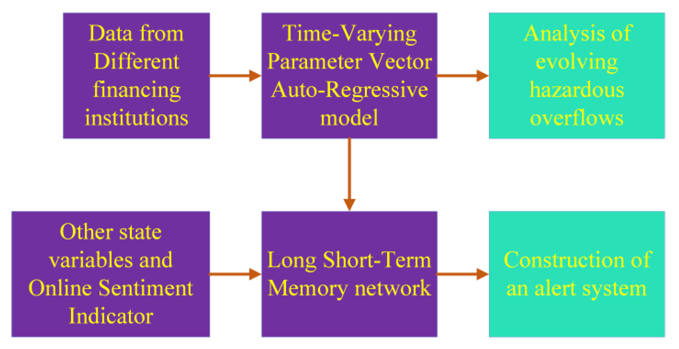
Figure 1. The overall sketch.
Mathematics 11 03279 g001
Figure 2. The recurrent unit structure in LSTM.
Mathematics 11 03279 g002
Figure 3. Time-series plot of volatility for the banking industry.
Mathematics 11 03279 g003
Figure 4. Time-series plot of volatility for the insurance industry.
Mathematics 11 03279 g004
Figure 5. Time-series plot of volatility for the securities industry.
Mathematics 11 03279 g005
Figure 6. Time-series plot of volatility for the diversified financial industry.
Mathematics 11 03279 g006
Figure 7. Time-series plot of hazard overflows in the financial system.
Mathematics 11 03279 g007
Figure 8. Time-series plots of hazardous exposures in the different finance industries. (a) Banking industry. (b) Insurance industry. (c) Securities industry. (d) Diversified financial industry.
Mathematics 11 03279 g008aMathematics 11 03279 g008b
Figure 9. Time-series plots of hazard overflows in the different finance industries. (a) Banking industry. (b) Insurance industry. (c) Securities industry. (d) Diversified financial industry.
Mathematics 11 03279 g009aMathematics 11 03279 g009b
Figure 10. Time-series plots of net overflows in the different finance industries. (a) Banking industry. (b) Insurance industry. (c) Securities industry. (d) Diversified financial industry.
Mathematics 11 03279 g010
Figure 11. Time-series plots of net overflows between the two finance industries. (a) Banking Versus Insurance. (b) Banking Versus Securities. (c) Banking Versus Diversified finance. (d) Insurance Versus Securities. (e) Insurance Versus Diversified finance. (f) Securities Versus Diversified finance.
Mathematics 11 03279 g011aMathematics 11 03279 g011b
Figure 12. Learning results of LSTM. (a) The training. (b) The testing.
Mathematics 11 03279 g012
Figure 13. Learning results of ANN. (a) The training. (b) The testing.
Mathematics 11 03279 g013
Figure 14. Learning results of SVM. (a) The training. (b) The testing.
Mathematics 11 03279 g014
Figure 15. Learning results of DT. (a) The training. (b) The testing.
Mathematics 11 03279 g015aMathematics 11 03279 g015b
Figure 16. Learning results of RF. (a) The training. (b) The testing.
Mathematics 11 03279 g016
Figure 17. OSI from 2010 to 2022.
Mathematics 11 03279 g017
Table 1. The most related literatures.
LiteratureBaselineStateHazardous
Overflow
Hazardous Alert
López et al. [1]Conditional value-at-riskFailure to consider the interdependence and volatility characteristics between financial relevant time-series data×
Derbali et al. [2]Marginal expected shortfallDitto×
Engle et al. [3]Coefficient of systemic financial hazard Ditto×
Wu et al. [4]Time-varying generalized auto-regressive conditional heteroscedasticity modelN/A×
Wu et al. [4]Rolling window dynamic Copula methodN/A×
Cao et al. [5]Variance decomposition & Rolling window Information loss×
Zhao et al. [7]Time-varying parameter vector auto-regressiveInformation loss×
Ni et al. [8]Weighted networkN/A×
Yang et al. [9]TENETN/A
Wang et al. [11]Factor hazard modelLack of interpretability for financial time-series data×
Wang et al. [11]Stochastic time-varying modelDitto×
Wang et al. [16]Machine learningPoor generalization×
Zhang et al. [18,19]Average stochastic gradient descent and weight-dropped LSTMN/A×
Table 2. Table of hazard overflow formulations.
Industries & Indicators12mIn-Degree
1 d ˜ 11 , t d ˜ 12 , t d ˜ 1 m , t S 1 , t f r o m
2 d ˜ 21 , t d ˜ 22 , t d ˜ 2 m , t S 2 , t f r o m
m d ˜ m 1 , t d ˜ m 2 , t d ˜ m m , t S m , t f r o m
Out-degree S 1 , t t o S 2 , t t o S m , t t o
Net overflowNet1,tNet2,tNetm,tFHOt
Table 3. Financial list and ID.
IDsInstitutionsIndustries
1Ping An BankBanking
2Bank of NingboBanking
3Pudong Development BankBanking
4Hua Xia BankBanking
5Minsheng BankBanking
6Merchants BankBanking
7Bank of NanjingBanking
8Industrial BankBanking
9Bank of beijingBanking
10Bank of CommunicationsBanking
11Industrial and Commercial BankBanking
12China Construction BankBanking
13Bank of ChinaBanking
14China Citic BankBanking
15China Pacific InsuranceInsurance
16China Life InsuranceInsurance
17Ping An InsuranceInsurance
18Northeast SecuritiesSecurities
19Guoyuan SecuritiesSecurities
20Changjiang SecuritiesSecurities
21Citic SecuritiesSecurities
22Sinolink SecuritiesSecurities
23Southwest SecuritiesSecurities
24Sunny Loan TopSecurities
25Everbright SecuritiesSecurities
26Shaanxi International Trust ADiversified finance
27New huangpuDiversified finance
28Henan Zhongyuan expresswayDiversified finance
29Haide LimitedDiversified finance
30Tianmao GroupDiversified finance
Table 4. Quantitative descriptions of volatility in different financial industries.
StatisticsBankingInsuranceSecuritiesDiversified Finance
Sample size2792279227922792
Mean26.0932.7538.9740.52
Standard deviation15.6017.6322.4418.95
Median21.8428.3532.8535.75
Maximum7.286.631.426.88
Minimum177.14163.97197.82187.50
Table 5. Financial hazard alert indexes.
IndexesDescriptions
Financial hazard overflow (FHO)The financial industry’s own hazard overflow indicator
Logarithmic return of the Shanghai Composite Index
(LR)
The daily closing price logarithmic return
Volatility of the Shanghai Composite Index
(VO)
The difference between the daily highest price and the daily lowest price
Short-term liquidity spread
(SLS)
The spread between the 6-month SHIBOR(Shanghai Interbank Offered Rate) and the 6-month government bond yield
Interest rate hazard
(IRH)
The spread between the pre- and post-maturity yields of the 6-month government bonds.
Interest rate term structure
(IRTS)
The difference between the 6-month government bond yield and the 10-year government bond yield at time period t, minus the difference between the 6-month government bond yield and the 10-year government bond yield at time period t − 1
Real estate yield
(REY)
Daily closing price logarithmic return
Table 6. LSTM model structure and parameters used in this paper.
StructureParameters
InputTime step5
→ LSTM layerPrediction step1
→ LSTM LayerNumber of iterations600
→ Dropout layerOptimizerAdam
→ Full Connection layerDropout rate0.01
→ OutputLoss functionMSE
Activation functionTanh
Batch_size30
Number of hidden layer neurons50
Proportion of test set0.25
Table 7. Nonlinearity test of variables.
Null HypothesisStatistics
FHO is not the cause of LR1.699 **
LR is not the cause of FHO1.483 *
FHO is not the cause of VO0.781
VO is not the cause of FHO1.480 *
FHO is not the cause of SLS1.743 **
SLS is not the cause of FHO1.780 *
FHO is not the cause of IRH1.311 *
IRH is not the cause of FHO1.407 *
FHO is not the cause of IRTS1.460 *
IRTS is not the cause of FHO0.041
FHO is not the cause of REY2.490 ***
REY is not the cause of FHO1.778 **
Note: *, **, and *** represent significance at the 0.1, 0.05, and 0.01 levels, respectively.
Table 8. Error results of LSTM.
ErrorTraining SetTesting Set
MAE0.08950.0957
MSE0.00860.0230
Table 9. Error results of other machine learning models.
ModelsMetricsTraining Set Testing Set
ANNMAE0.33020.3422
MSE0.30410.3465
SVMMAE0.80470.8366
MSE1.39931.4089
RFMAE0.12660.3431
MSE0.04780.3346
DTMAE1.57511.5377
MSE3.67233.5053
Table 10. Error results of all models in the ablation experiment about OSI.
ModelsMetricsTraining SetTesting Set
LSTMMAEa0.08950.0957
MAEb0.05720.0865
MSEa0.00860.0230
MSEb0.00390.0256
ANNMAEa0.33020.3422
MAEb0.29910.3106
MSEa0.30410.3465
MSEb0.27160.3200
SVMMAEa0.80470.8366
MAEb0.79630.8345
MSEa1.39931.4089
MSEb1.38671.4146
RFMAEa0.12660.3431
MAEb0.12560.3350
MSEa0.04780.3346
MSEb0.04660.3389
DTMAEa1.57511.5377
MAEb1.57511.5377
MSEa3.67233.5053
MSEb3.67233.5053
Disclaimer/Publisher’s Note: The statements, opinions and data contained in all publications are solely those of the individual author(s) and contributor(s) and not of MDPI and/or the editor(s). MDPI and/or the editor(s) disclaim responsibility for any injury to people or property resulting from any ideas, methods, instructions or products referred to in the content.