Resolving the Doubts: On the Construction and Use of ResNets for Side-Channel Analysis

Abstract

The deep learning-based side-channel analysis gave some of the most prominent side-channel attacks against protected targets in the past few years. To this end, the research community’s focus has been on creating the following: (1) powerful multilayer perceptron or convolutional neural network architectures and (2) (if possible) minimal multilayer perceptron or convolutional neural network architectures. Currently, we see that, computationally intensive hyperparameter tuning methods (e.g., Bayesian optimization or reinforcement learning) provide the best results. However, as targets with more complex countermeasures become available, these minimal architectures may be insufficient, and we will require novel deep learning approaches.This work explores how residual neural networks (ResNets) perform in side-channel analysis and how to construct deeper ResNets capable of working with larger input sizes and requiring minimal tuning. The resulting architectures, obtained by following our guidelines, are significantly deeper than commonly seen in side-channel analysis, require minimal hyperparameter tuning for specific datasets, and offer competitive performance with state-of-the-art methods across several datasets. Additionally, the results indicate that ResNets work especially well when the number of profiling traces and features in a trace is large.

1. Introduction

Many digital devices, from phones to payment terminals, rely on encryption algorithms for security. While modern cryptographic algorithms are (presumed to be) theoretically secure, the practical implementations come with an entirely separate set of concerns. Several types of attacks that rely on some vulnerability in the implementation exist. In this work, we focus on side-channel analysis (SCA). Side-channel analysis is a non-invasive implementation attack, focusing on extracting leaked information during the algorithm’s execution. Examples of these leakages include the following: timing [1], power consumption [2], electromagnetic emanation [3], sound [4],or cache-timings [5].

In the last few years, the focus of the side-channel community has primarily shifted to attacks using deep learning techniques [3,6,7]. Various works have looked at different neural network architectures and hyperparameter setups. Still, the general trend for state-of-the-art performance has been to take relatively small architectures [8] and to use automated techniques to find optimal hyperparameter configurations [9,10]. While some works have explored deeper architectures for specific scenarios, such as attacking traces with large feature windows [11,12] or desynchronized traces [13,14], these cases are relatively limited when compared to the large number of works using smaller architectures [8,9,10,15,16,17,18].

Although targets protected with various countermeasures have become relatively straightforward to break with deep learning techniques [8,16], there are newer datasets that seem more difficult to successfully attack [12]. These recent datasets commonly provide more measurements (and features) for the profiling and the attacking phase. As a result of the increased complexity of the datasets, due to the additional countermeasures, larger architectures may provide a way to break these targets. Therefore, it is essential to provide insights into the construction and performance of these larger architectures to make any conclusions as to the viability of the architectures for such tasks.

Since we focused on deeper neural networks, we used Residual networks (ResNets). The ResNets are neural network architectures that include shortcut connections between network layers. As these shortcut connections are added in deep networks, updating the weights in earlier layers becomes difficult as the gradient vanishes in the deeper layers. The shortcut connections then allow the gradient to skip layers and let the weights in these deeper layers be trained [19]. The benefit of ResNets in this context is that the residual connections allow deeper networks to be used without running into gradient vanishing issues. Additionally, some recent works have used ResNets for side-channel analysis and have shown promising results [14,20].

1.1. Related Work

Recently, several works investigated ResNets and concluded that they have relatively competitive performances with the state-of-the-art SCA. Zhou and Standaert explored using a ResNet architecture for dealing with desynchronized traces and showed impressive attacking results [14]. Jin et al. also showcased a ResNet architecture utilizing attention mechanisms, and the resulting architectures performed well across a fairly wide variety of datasets [20].While both of these works showed good attacking results using ResNets, how the authors arrived at the architectures they used is unclear. There are no experimental results that investigate the benefits (or downsides) of fundamental design choices in the construction of ResNet architectures and, as such, it is unclear whether the architectures used are optimal. Additionally, these works do not provide a clear basis to compare the performance of ResNet architectures to other state-of-the-art methods. In [20] it is difficult to understand how much of the performance improvements should be attributed to the use of the attention-based mechanisms, and in [14] the main focus is on non-public datasets and the architecture description is unclear and does not allow the reproduction of the results. Next, Gohr et al. used ResNets to break the CHES CTF 2018 dataset, exploring deeper networks with up to 19 residual blocks [21]. The authors also discussed breaking the full key and not only one subkey guess, as is commonly done. Finally, Masure et al. did not use ResNets, but discussed them, and concluded that it is possible to use distinctive features in SCA traces and avoid problems connected with deep architectures (which would then necessitate the usage of ResNets) [22].

Other works have looked at attacking datasets with large numbers of features. Lu et al. attacked the raw traces of several datasets with novel, attention-based architectures and showed impressive results [11]. The authors also required large neural network architectures for this. Indeed, they used architectures with more than 50 layers, while most of the results in the SCA domain are accomplished with architectures with less than ten layers. Perin et al. also explored various feature selection scenarios and showed that even very small architectures could have excellent results against datasets with large numbers of features [18]. Moreover, the authors showed that it is possible to break the targets in certain cases with only a single attack trace. Finally, Masure et al. looked at how the code–polymorphism countermeasure impacts the security of implementations against attacks using deep learning [22]. This countermeasure results in large feature windows, as the sensitive operations are spread across larger periods of time. As a result of this, Masure et al. created adapted CNN-like architectures to deal with these large-scale traces.

We can make several observations when we look at the state-of-the-art methods for attacking more commonly used datasets in SCA. The architectures proposed by Zaid et al. are amongst the top-performing architectures for several datasets [8]. These small architectures provide a base for the novel model search strategies currently providing top performance for various datasets. Wu et al. showed how Bayesian optimization could be used to optimize the hyperparameters for small architectures for specific datasets [10]. They also found that random search can perform well if the hyperparameter search ranges are adequately limited. Rijsdijk et al. utilized reinforcement learning to generate top-performing architectures automatically [9]. More recently, Schijlen et al. explored an approach, based on genetic algorithms, that performs competitively with the aforementioned approaches [17]. Furthermore, Acharya et al. showed that an information theoretic approach performs competitively while reducing computational overheads, in terms of memory footprint and time complexity [15]. These automated search techniques rely on training and evaluating large numbers of models and on pre-selecting reasonable ranges for hyperparameters to limit the otherwise unreasonable search ranges.

Finally, there are some works that look at utilizing the benefits of DL-based approaches for non-profiled attacks. Timon showed that, by training networks for each possible key candidate it is possible to distinguish the correct key [23]. To mitigate the significant computational overheads of training a model for each key candidate, Do et al. proposed a multi-output regression approach to train only one neural network. More recently, methods using DL networks trained on plaintext labels have been used to directly mount attacks [24] and to improve collision attacks [25].

1.2. Our Contributions

This paper investigates how ResNets can be used in SCA and, more precisely, how difficult it is to tune them and how they compare with state-of-the-art results. Our main contributions follow:

• We empirically investigate several constructions for deep ResNets and provide recommendations about what type of residual block should be used and how deep the networks should be for state-of-the-art side-channel analysis.
• From these recommendations, we construct a novel architecture that is significantly deeper than the architectures previously used for SCA. This architecture performs competitively with state-of-the-art model search strategies across several datasets. In several settings, we obtained the best-known results (compared with other types of deep learning and the same number of features).

2. Background

2.1. Deep Learning

Deep learning (DL) is a form of machine learning (ML) where the algorithm to learn the function is a neural network of interconnected layers. Such DL algorithms are generally (in the context of SCA) used to perform classification in a supervised learning setting. A supervised learning setting is a setting where a set of already-labeled data is taken, and a model is created from this labeled data to predict the labels for data that have not been used before [26].

As described above, DL networks are trained using a set of training data assigned with classification labels. The training lasts for a number of epochs. One epoch is equivalent to processing all training data once (forward and backward passes with the backpropagation algorithm). The data is divided into batches, and each batch is utilized in one iteration. When the network has generated predictions for a batch, the models’ predictions are compared to the actual labels. This comparison is made by computing a loss function. Various loss functions are used to measure the errors the networks make during classification. The goal during training is, then, to minimize the loss of the network. This is accomplished by computing the gradient of the loss function concerning the weights in the network. Then, the weights are updated according to this gradient by an amount scaled with the learning rate. Several methods exist for updating the weights, and we refer to these as optimizers.

2.2. Residual Neural Networks

A specific family of CNN architectures is that of Residual Neural Networks (ResNets). One of the main problems deep CNN architectures experience is the gradient vanishing problem wherein weights in the earlier layers of the network cannot be efficiently updated using the gradient, since the gradient is too small in these layers [27]. This gradient vanishing results in the training of very deep networks to be very complex [28]. To avoid this problem, ResNets have shortcut connections that skip over some of the layers in the network. These shortcut connections allow the network to have many layers while still not experiencing the problem of vanishing gradients. Often, ResNets are implemented using residual blocks. These are blocks of convolutional layers. Then, a shortcut connection is added to the output of the residual block. This connection allows the gradient to flow through the shortcut connection, which helps resolve the problems mentioned above (i.e., gradient vanishing). This shortcut connection is generally realized with a connection lacking any intermediate operations or a convolutional layer with kernels of size one, to match the number of filters for the addition. Examples of typical constructions of residual blocks can be seen in Figure 1.

2.3. Profiling Side-Channel Analysis

The setting we considered was the profiling side-channel analysis. Profiling attacks are generally more powerful than their non-profiling counterparts, as the adversary is assumed to have access to (and full control over) a copy of the device being attacked [29]. The main workflow for profiling SCA is to take a large number of measurements from the copy of the device and to create a model of its behavior. Generally, this is done by labeling all measurements using the chosen leakage model. A leakage model describes how the leakage depends on some sensitive internal state dependent on the key [2]. Labeling the traces with this leakage model is possible, as the adversary is assumed to have access to the key on the copied device. After the profile of the clone device is built, several measurements are taken from the device that is being attacked. A set of labels for these measurements is generated using each of the possible values for the key bytes, and, for each of these, the log-likelihood, according to the profile, is computed. In cases of a successful attack, the correct key byte has a high (ideally, the highest) log-likelihood [30].

Creating these profiles can be seen as a supervised learning task, as measurements are collected, labeled, and, then, used to train a model to predict new measurements. Over the past years, ML and DL approaches have become prevalent in profiling SCA. Specifically, the DL approach has led to impressive results, successfully attacking datasets protected by various countermeasures [7,8].

SCA Metrics

ML approaches for profiling SCA have proven very successful. However, accuracy and loss, often used in standard classification tasks, are not necessarily the best indicators of how successful a side-channel attack will be. While very good accuracy scores, or loss values, indicate a successful attack, this is not a necessary condition. Indeed, models that perform slightly better than random guessing can also generate successful attacks [31]. The models in profiling SCA are usually evaluated based on metrics related to the correct key’s rank. Here, the rank of the correct key is the number of key candidates with a higher log-likelihood than the correct key. Generally, metrics are computed using a relatively large number of attacks on random subsets of the full-attacking set to accurately depict the realistic (averaged) performance. More formally, we define the vector $g_{S_a}$ as a vector of key guesses ordered by the log-likelihood of each key. Here, $S_a\subset N_a$ is a subset of the full attacking set $N_a$. Then, we define $g_{S_a}\left(k\right)$ as the rank of a key candidate k. The two main metrics we considered were:

• Guessing Entropy: Guessing entropy (GE) [32] is the average key rank over a number of attacks. This is defined as $GE\left(N_a\right)=\mathbf{E}\left(g_{S_a}\left(k^{*}\right)\right)$, where $\mathbf{E}$ is the mean function. As is commonly done, we estimated it over 100 attacks.
• NoT: The NoT (Number of traces) metric refers to the number of measurements required to reduce GE to one (i.e., to see if our best guess was also the correct guess). This is defined as $min\left\{\right|N_a\left|\right\}$, for which $GE\left(N_a\right)=1$. Then, the NoT metric estimates how many measurements are required to recover the key.

2.4. Datasets

We ran our analysis on three datasets. They represented common choices when assessing the performance of deep learning-based SCA, and, as such, they have been used in numerous papers; see, for example, [7,8,16].

The ASCAD database [3] provides datasets from a protected AES implementation. The sensitive value attacked for these implementations is generally the output of the third S-box in the first round (as the third key byte is the first masked one). The ASCAD database provides traces measured on an AES implementation, implemented on the ATMega8515 device. This implementation is protected with the first-order masking scheme around the S-box, which can be described as:

$$S-box[p_i\oplus k_i]\oplus r_{out}.$$

Here, $p_i$ and $k_i$ represent the i-th byte of the plaintext and the key, respectively. $r_{out}$ represents the additive mask.

Two versions of this dataset are provided. The first dataset has 50,000 training traces and 10,000 attacking traces. All of the traces were measured with the same key and random plaintexts. These traces were 100,000 samples (features) long, and the authors provided a pre-selected window of 700 samples for attacking the third key byte for comparisons of attacks. We refer to this version as ASCADf.

The second dataset has 200,000 training traces and 100,000 attacking traces. The profiling traces were measured with random keys and plaintexts, and the attacking set had a fixed key. The traces were 250,000 samples long, and the authors provided a pre-selected window of 1400 samples for attacking the third key byte. We refer to this version as ASCADr.

The AES_HD dataset provides an unprotected AES hardware implementation [7]. The dataset was measured on a Xilinx Virtex-5 FPGA. The dataset contains 500,000 traces with 1250 features each [33]. As the implementation is hardware-based, there is significantly more noise present than is the case for the ASCAD datasets. Another difference is that a different leakage model is used for AES_HD. The writing of the output to the register in the final round being attacked:

$$InvSbox[C_i\oplus k*]\oplus C_j.$$

Here, $C_i$ and $C_j$ are two of the ciphertext bytes, and the relationship of i and j is based on the inverse ShiftRows operation. Generally, we used $i=16$ and $j=12$, as this is one of the easier bytes to attack [7]. Additionally, we used the Hamming distance of this resulting operation as the leakage model.

3. Construction of Deep ResNets for SCA

Our experiments were run on a high-performance computing cluster (HPC), and we used one NVIDIA GeForce GTX 2080Ti GPU with 11 GB of memory. The required amount of RAM ranged from sixteen to sixty-four GB of RAM, and training one of the models took from twenty minutes to two hours, depending on the dataset and model size. The AISY Framework [34] was used to implement the experiments with Python 3.7, TensorFlow 2.0, and Keras 2.1.6.

As we wished to determine whether ResNets could be a viable alternative for the more common smaller CNNs currently used in SCA, we first needed to create architectures specifically created for SCA. First, we needed to determine whether residual blocks worked well, which is a central part of our architecture. Second, it was helpful to determine how deep the architectures should be to mount successful attacks consistently.

3.1. Residual Block Construction

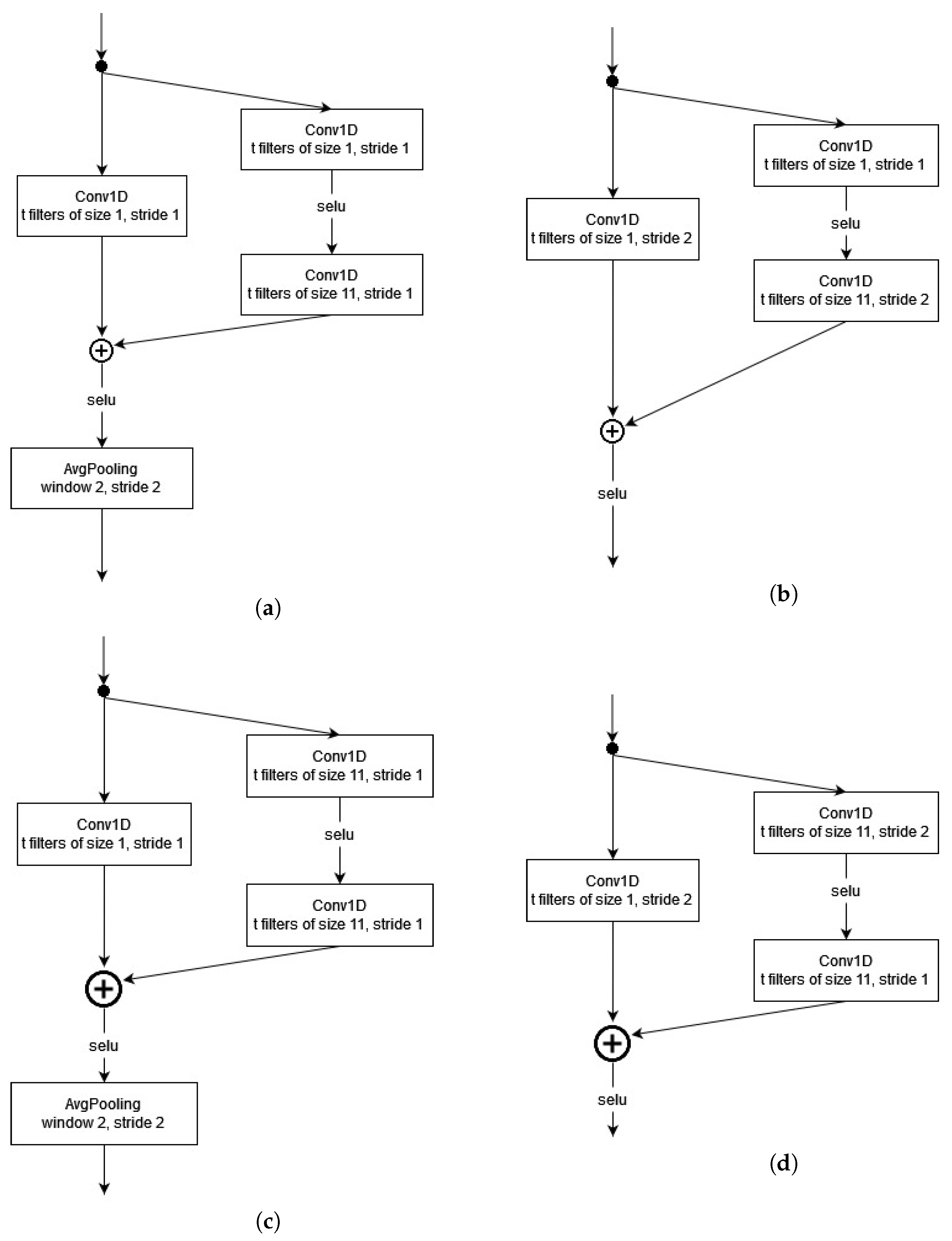
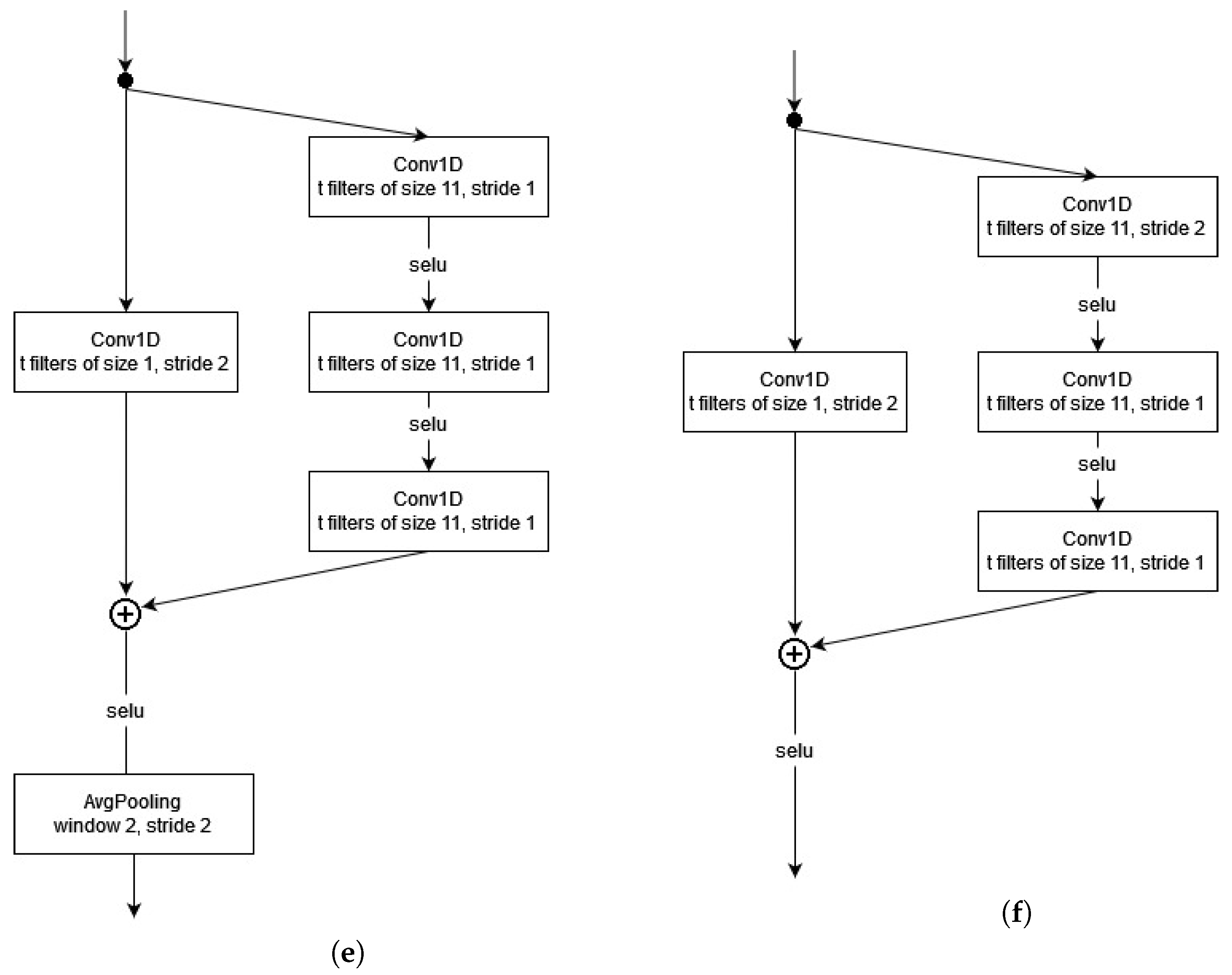
We chose an empirical approach to test how residual blocks should be constructed for SCA. We determined that there were six reasonable choices for the construction of the blocks. These choices were based on recent works that explored ResNets for SCA [14,20]. We also chose the Inception block, based on recent works in image recognition [35]. Inception blocks are residual blocks where the first convolutional layer has its kernel size set to one. They were included here because they could help mitigate the extra performance overheads of our deeper networks, while potentially not harming the attacking performance. The tested blocks can be seen in Figure 2. It is worth noting that we limited ourselves to a relatively small number of basic residual blocks. We chose to only look at relatively simple residual blocks because we wanted to determine what types of basic construction functioned well in deeper networks. Additionally, we supposed that even simpler blocks could provide good attack performance. In that case, it was intuitive that, with more experiments, it would be wcwn further possible to improve the results and adjust for specific datasets and settings.

To limit the scope of our search for the best residual block, we decided that each block should include either a convolutional stride or a pooling layer, so as to reduce the feature map size by half. This design decision was made since the earlier ResNets in SCA also used such blocks [12,14,20], and the reduction in feature map size in the network has been a standard in some of the state-of-the-art architectures in SCA [7,8]. This choice limited the maximum number of residual blocks our network could contain. This maximum was determined by the number of features, and it equaled $\lfloor lo{g}_2\left(700\right)\rfloor =9$ (for the ASCADf dataset).

To test the blocks, we attacked the ASCADf dataset with the pre-selected window of 700 features. We used 50,000 traces for training and 5000 traces for both validation and attacking. The network we used can be seen in Figure 3. The filter size was 11, and the number of filters in the i-th residual block equaled min(2${}^{i-1},256)$. The activation function was selu, and the optimizer was the Adam [36] optimizer with a cyclic learning rate schedule [37]. The loss function we used was categorical cross-entropy. We used 100 epochs and a batch size of 50. We chose these hyperparameter values based on the work of Zaid et al. [8]. While they were not necessarily optimal, it was reasonable to assume good enough performance to test the differences in the performances the various residual blocks could achieve.

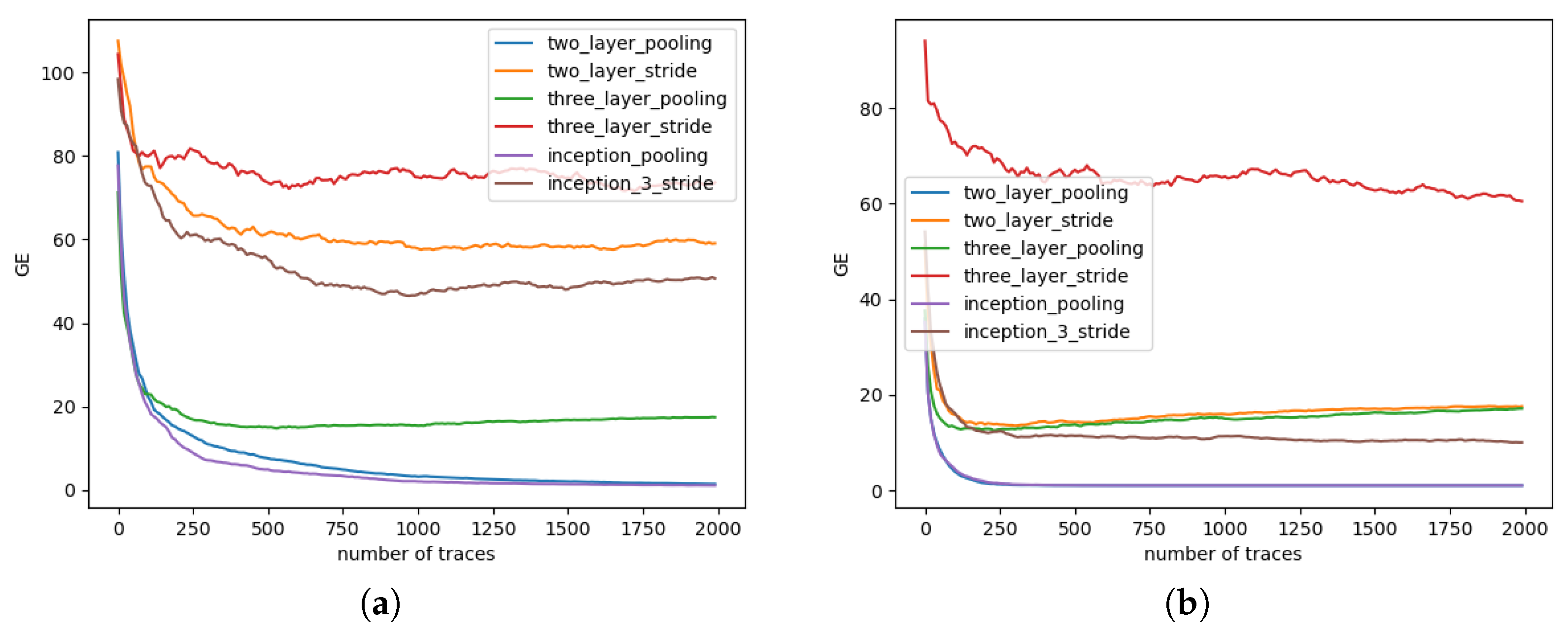
To verify that the networks performed consistently, all of the results in this section were averages over five training runs of the network. Additionally, GE was computed as an average of 100 attacks. Finally, during training, we saved the model that achieved the best validation loss, and we tracked the number of attacking traces required to reach GE = 1. In Figure 4, it can be observed that the average attacking performance of the models with each residual block was significantly worse after the entire 100 epochs, than it was if the model with the best validation loss was used instead. This performance difference was due to the size of the tested networks being larger than necessary for the dataset. Due to this, we observed that the models overfitted, as can also be seen in Figure 5. Additionally, we observed that the models using pooling for feature map size reduction consistently performed better than those using convolutional stride. We believe this might be because when a convolutional stride was used (Stride controls the amount of movement over the data. The larger the stride, the more downsampling of the data.), specific patterns might be skipped over in the convolutions. Skipping these patterns could result in specific leakage points being missed entirely, resulting in worse performance. Finally, we observed that the two_layer_pooling- and the inception_pooling blocks performed best out of the chosen residual blocks, with the difference in attacking performance between these two being negligible.

In Figure 5, another reaffirmation of the earlier results can be observed. We again see that, generally, the two_layer_pooling- and the inception_pooling blocks performed significantly better than their counterparts, in terms of the number of traces required to reach GE = 1. When we look at the validation loss, we note that there was no large difference between the various blocks using pooling. However, we again observe that pooling layers were better than convolutional stride.

3.2. Depth of ResNets

We conducted experiments that varied the number of residual blocks to test how deep our Resnets should be for SCA. Varying these blocks was straightforwardly accomplished; the only notable exception was that, now, we excluded the pooling layer from the final residual block. This was done as a GlobalAveragePoolingLayer immediately following this block, and, therefore, including a pooling layer in the final block was pointless. For these experiments, we only used the two_layer_pooling residual block to limit the number of experiments that we had to run. We chose this residual block as it was one of the two best-performing residual blocks in our earlier experiments. All other hyperparameters were identical to the earlier experiments, and the network setup was the same as that in Figure 3, except for the number of residual blocks.

In Figure 6, we see that adding residual blocks seemed to improve the attacking performance of the networks up to a point. From 4 to 7 residual blocks, the best models steadily improved the attacking results. The difference from 7 to 9 residual blocks was negligible. The results were similar for models after the full 100 epochs.

We see some of the same phenomena when we look at the progression of the validation metrics across the epochs in Figure 7. The networks with 4 to 6 residual blocks seemed to perform a fair bit worse than those with 7 or more residual blocks. Specifically, in regard to the validation loss, the networks with 9 residual blocks performed slightly better than the rest, but this did not seem to translate into improved attack performance, as observed in Figure 6.

Combining all of these results provided several observations. First, using pooling layers over a convolutional stride looked like an obvious choice, as the performance difference was significant. This differed from several of the other ResNets in SCA [12,14], which suggested that these architectures could be improved significantly with this substitution. Second, using more than two convolutional blocks did not look useful in our experiments, and, thus, we chose to use the two-layer block in the next section. Still, the Inception version was a viable alternative. Finally, we showed that using more residual blocks helped the performance of the models for SCA, up to a point. Our experiments showed that using more than seven residual blocks did not improve performance. If we generalize this, when a dataset has x features, using $\lfloor lo{g}_2\left(x\right)\rfloor -y$ residual blocks seem a reasonable choice as using more residual blocks results in an additional computational overhead, while, as evidenced in our experiments, not improving performance. Our experiments showed that $y=2$ provided reasonable results, but more experiments are needed before giving definitive recommendations. Still, we consider it “safe” to recommend that y should be a small value (e.g., 1 or 2).

4. Comparison With State-of-the-Art CNN and MLP Architectures

We explored how ResNets should be constructed for SCA to provide insights into what types of residual blocks function well and how deep the ResNets should be. However, it is still unclear how well ResNets compare to other state-of-the-art DL approaches. Therefore, we do not yet know whether ResNets can be a viable alternative and, if they are, in what scenarios.

To remedy this, we aim to utilized the ResNets we developed to attack the AES_HD dataset and both versions of the ASCAD datasets. These experiments enabled us to reach conclusions about the efficacy of ResNets in scenarios with varying numbers of profiling traces and for both protected software and unprotected hardware implementations. Additionally, it allowed us to directly compare the results of our ResNets to the results of state-of-the-art model search strategies of Perin et al. [18] on the ASCAD datasets and to the state-of-the-art CNN architecture of Zaid et al. [8] on the AES_HD dataset. The architectures we compared against from [18] were the best-achieved MLP and CNN models for each dataset, using the ID leakage model in the OPOI scenario. OPOI represents the optimized points of interest setting, where the attacked dataset consists of an optimized interval, including the main SNR peaks and several low SNR points. This scenario is commonly considered in related works, see, for example, [8,38]. In our experiments, we only considered the Identity leakage model.

The experimental setup for the ASCAD datasets was similar to the one used in the previous section. We used 50,000 and 200,000 profiling traces for ASCADf and ASCADr, respectively. For both ASCAD datasets, we used 5000 traces for validation and 5,000 traces for attacking, and we used the standard 700 and the 1 400 feature intervals. For the AES_HD dataset, we used 50,000 profiling traces and 12 500 validation and attacking traces. Our hyperparameter setups in this section were generally the same as in Section 3. Two minor changes to the hyperparameters were made for AES_HD and ASCADr. For AES_HD, we used a kernel size of 3 as opposed to 11 to emphasize “smaller” details that were to be expected, due to more noise and the hardware implementation. For ASCADr, we used 200 neurons in both of the fully connected layersm as opposed to 10. This was because, with the additional training examples this dataset contained, we could use more neurons in these final layers without the network immediately overfitting. Thus, these additional neurons allowed our network to mount more powerful attacks. We again saved the model weights that resulted in the best validation loss during training and presented the result of this model. The number of residual blocks we used for each dataset depended on the number of features. We used $\lfloor lo{g}_2\left(\mathrm{num}\_\mathrm{features}\right)\rfloor -2$ residual blocks for each dataset as was recommended in Section 3. This resulted in 7 residual blocks for ASCADf and 8 residual blocks for both ASCADr and AES_HD. For the ASCAD datasets, we also attacked larger intervals of varying sizes around the optimized intervals. These experiments were used to evaluate the impact of more features on the performance of our ResNets. The indices of an interval of size x were then $[45750-(x/2),45750+(x/2\left)\right]$ for ASCADf, and $[81645-(x/2),81645+(x/2\left)\right]$ for ASCADr. It should be noted that the larger feature sets here included additional leakage points, andm as such, attacks against larger windows could achieve better attack results. We took the best-performing model out of five training runs to compare our models to the state-of-the-art. Training the model several times is conducted, as models are often inconsistent and do not always converge, and, in the literature, the best-case performance is commonly showcased.

4.1. Results

ASCADf. When we compared our results to the state-of-the-art results from [18], we observed that our results were somewhat worse. Indeed, we required almost double the number of traces for CNN and 50% more traces than MLP. However, the attack results for our ResNets were still reasonable, especially considering that we had made limited investigations into optimizing our hyperparameter configurations. We believe that the performance gap we saw here could potentially be bridged with enough additional tuning. Another insight, that can be observed in

Table 1. Comparing the performance and size of our ResNets against the models resulting from state-of-the-art model search strategies on ASCADf.

	ResNet	CNN [18]	MLP [18]
Nr. of traces to reach GE = 1	160	87	104
Nr. of trainable parameters	96,800	7728	10,266

, was the number of trainable parameters for each architecture. Our ResNets had a significantly higher number of trainable parameters than the relatively small architectures required in [18]. This additional size was unnecessary for this dataset and resultws in our network starting to overfit in the first half of the training. As we saved the model with the best validation loss, the performance penalty from this overfitting was mitigated.

ASCADr. When we compared the ResNets to the state-of-the-art results in

Table 2. Comparing the performance and size of our ResNets against the models resulting from state-of-the-art model search strategies on ASCADr.

	ResNet	CNN [18]	MLP [18]
Nr. of traces to reach GE = 1	47	78	129
Nr. of trainable parameters	489,592	87,520	34,236

, it can be observed that the results of our networks were better than the hyperparameter search strategy of Perin et al. [18]. Surprisingly, our models outperformed the methods here, as the model search found a model tuned specifically for this dataset. We expected our model to perform slightly worse than the state-of-the-art, as was the case for ASCADf. We presume this difference was because the models were trained with a significantly larger training set than for ASCADf. As a result of this, our deeper models could learn a better profile, while the smaller networks that resulted from model search techniques did not benefit from the additional information as much. An additional consideration here is that training the final models of [18] only took a few minutes, while training the larger ResNet took about 1.5 h for this dataset. The improved attacking performance came at a relatively high computational cost. However, ref. [18] trained and evaluated 500 models to find these networks. Training these models can take a couple of hours to complete, or, if the search space also includes bigger models, it can take several days. When we consider this, the additional cost to train one of our ResNet models is justified, as it minimizes the extensive search for optimal hyperparameters (still, we note that we also required limited tuning to find our architecture). In

Table 3. Comparing the number of traces required to reach GE = 1 at various feature selection scenarios for both ASCADf and ASCADr.

Nr. of Features	Nr. of Residual Blocks	ASCADf	ASCADr
1500	8	36	34
2000	8	64	37
2500	9	86	37
3000	9	42	29
3500	9	6	21
4000	9	10	14
4500	10	9	9
5000	10	10	8

, we provide additional results for ASCAD datasets that show more features are beneficial in regard to the performance of ResNets, giving an additional argument in their favor. Notice how we found a setting where we required less than ten traces to break the target for both datasets. Finally, our recommendation on the required number of residual blocks generalized well for the tested cases.

AES_HD. When attacking the AES_HD dataset, we observed some interesting phenomena. It can be observed in

Table 4. Comparing the performance and size of our ResNets against resulting state-of-the-art CNN model AES_HD.

	ResNet	CNN [8]
Nr. of traces to reach GE = 1	4100	6060
Nr. of trainable parameters	111,491	3278

that the ResNet could successfully recover the key in approximately 4100 attack traces. This attack was significantly better than the state-of-the-art CNN model of Zaid et al., which could recover the key in about 6060 traces. It is worth noting that the Zaid et al. network trains in only a few minutes, while training our network takes approximately half an hour. Additionally, our model has significantly more trainable parameters.

4.2. Discussion

Our experiments to determine the advisable residual block constructions showed that models using convolutional stride perform significantly worse than models using pooling layers. We believe this can be attributed to the fact that, when a convolutional stride is used, specific patterns might be skipped over in the convolutions. Furthermore, using more than two convolutional layers per residual block seems to worsen the attack performance of the models. Therefore, our experiments indicate that using residual blocks with two convolutional layers and a pooling layer, to reduce the feature map size, is the best choice for deeper ResNets in SCA. This result is in line with the work of Jin et al. [20]. The residual block they used adhered to these guidelines, but the focus of that work was the addition of attention mechanisms to these blocks. On the other hand, further recent uses of ResNets for SCA did not adhere to our guidelines. Masure et al. used convolutional stride [12], and Zhou and Standaert used residual blocks with three convolutional layers [14]. This leads us to believe that these works could be improved by updating the networks, as our results indicated that some of their design choices could negatively impact the attack performance.

The second main result is that deeper variants of our networks showed significantly improved attack results over the shallower variants. Our results indicated that adding residual blocks does not negatively impact attack performance and, indeed, improves it up to a point. We see that the networks that performed the best in our experiments were deeper than some of the other ResNets used for SCA [14,20] (Masure et al. used a network of similar depth, but the dataset they attacked had significantly more features [12]). The networks were also significantly deeper than those used in state-of-the-art works [8,9,18]. Recently, the general trend has been to utilize hyperparameter search strategies to find small architectures that perform well. These search methods involve running large numbers of models across predefined ranges of hyperparameters. These ranges are often (loosely) based on the work of Zaid et al. [8], which outlines a methodology for constructing relatively small architectures with excellent attack performance for specific SCA datasets. As a consequence of this, and because smaller architectures train faster, which makes training large numbers of them less cumbersome, the resulting architectures are often very shallow. This has resulted in a trend of very small architectures continually improving the state-of-the-art. Thus, while we showed reasonable results, we used hyperparameter setups designed for significantly smaller networks. It seems reasonable to assume that even better performance is expected with a more fine-tuned setup.

The ResNet attack performance is competitive with the state-of-the-art CNNs and is achieved across various datasets. It is also worth emphasizing that a single architecture (with minor variations, such as in the number of residual blocks used across these scenarios, or the kernel size and the number of neurons in the fully connected layers) is comparable to random search methods that result in varying model architectures and hyperparameter configurations. Additionally, while training ResNets is more computationally expensive than current state-of-the-art architectures [8], it is significantly faster than the model search strategies. Training one of the ResNets could take up to two hours in the scenarios tested here, which is a significant step up from the mere minutes it takes to train the small CNNs and MLPs that resulted from the searches. However, hundreds of models need to be trained and evaluated during the search for this specific architecture, which can take several hours or days to complete [9]. Additionally, the resulting architectures cannot be easily repurposed for different attack scenarios, while the ResNets only require minimal adjustments to be adapted (thus, they “generalize” better). The main use case for ResNets in SCA seems to be with larger datasets (both in terms of profiling set size and the number of traces). We observed that the networks performed significantly better when the ASCADr dataset was used, as opposed to the ASCADf dataset. Additionally, it is relatively intuitive that our larger networks can fit more complex models and are, therefore, more suited to more complex tasks with more training data. With new and more protected targets (where the measurements are also significantly larger), like AES_HD_mm [13] and the new ASCAD dataset [12], presumably becoming the focus of the SCA community in the coming years.

5. Conclusions and Future Work

This work developed and evaluated novel ResNet architectures for SCA. We conducted several experiments to determine suitable constructions for residual blocks and established how deep the networks should be. With these novel architectures, we attacked the ASCAD datasets and the AES_HD dataset. Our ResNets are competitive with state-of-the-art model search strategies and even surpass previous best results for the ASCADr dataset. Thus, we can conclude that ResNets provide an interesting new avenue for future research in SCA, especially if considering large datasets (i.e., with many features or training traces) and those protected with countermeasures. As our networks provide competitive performance without much hyperparameter tuning, this leads us to believe not only that more tuning can result in better performance, but also that limited tuning can still be a powerful option for diverse settings/datasets. Additionally, deeper ResNets could provide a way to attack more difficult targets that current deep learning state-of-the-art cannot break. For instance, the ASCADv2 [12] could be an interesting target to explore in future work.

References

1. Kocher, P.C. Timing attacks on implementations of Diffie-Hellman, RSA, DSS, and other systems. In Advances in Cryptology—CRYPTO’96: Proceedings of the 16th Annual International Cryptology Conference, Santa Barbara, CA, USA, 18–22 August 1996; Springer: Berlin/Heidelberg, Germany, 1996; pp. 104–113. [Google Scholar]
2. Kocher, P.; Jaffe, J.; Jun, B. Differential power analysis. In Advances in Cryptology—CRYPTO’99: Proceedings of the 19th Annual International Cryptology Conference Santa Barbara, CA, USA, 15–19 August 1999; Springer: Berlin/Heidelberg, Germany, 1996; pp. 388–397. [Google Scholar]
3. Benadjila, R.; Prouff, E.; Strullu, R.; Cagli, E.; Dumas, C. Deep learning for side-channel analysis and introduction to ASCAD database. J. Cryptogr. Eng. 2020, 10, 163–188. [Google Scholar] [CrossRef]
4. Anand, S.A.; Saxena, N. Anand, S.A.; Saxena, N. A sound for a sound: Mitigating acoustic side channel attacks on password keystrokes with active sounds. In Financial Cryptography and Data Security: Proceedings of the 20th International Conference, FC 2016, Christ Church, Barbados, 22–26 February 2016; Springer: Berlin/Heidelberg, Germany, 2016; pp. 346–364. [Google Scholar]
5. Yarom, Y.; Falkner, K. FLUSH+ RELOAD: A high resolution, low noise, L3 cache side-channel attack. In Proceedings of the 23rd {USENIX} Security Symposium ({USENIX} Security 14), San Diego, CA, USA, 20–22 August 2014; pp. 719–732. [Google Scholar]
6. Maghrebi, H.; Portigliatti, T.; Prouff, E. Breaking cryptographic implementations using deep learning techniques. In Security, Privacy, and Applied Cryptography Engineering: Proceedings of the 6th International Conference, SPACE 2016, Hyderabad, India, 14–18 December 2016; Springer: Berlin/Heidelberg, Germany, 2016; pp. 3–26. [Google Scholar]
7. Kim, J.; Picek, S.; Heuser, A.; Bhasin, S.; Hanjalic, A. Make Some Noise. Unleashing the Power of Convolutional Neural Networks for Profiled Side-channel Analysis. IACR Trans. Cryptogr. Hardw. Embed. Syst. 2019, 2019, 148–179. [Google Scholar] [CrossRef]
8. Zaid, G.; Bossuet, L.; Habrard, A.; Venelli, A. Methodology for Efficient CNN Architectures in Profiling Attacks. IACR Trans. Cryptogr. Hardw. Embed. Syst. 2020, 2020, 1–36. [Google Scholar] [CrossRef]
9. Rijsdijk, J.; Wu, L.; Perin, G.; Picek, S. Reinforcement Learning for Hyperparameter Tuning in Deep Learning-based Side-channel Analysis. IACR Trans. Cryptogr. Hardw. Embed. Syst. 2021, 2021, 677–707. [Google Scholar] [CrossRef]
10. Wu, L.; Perin, G.; Picek, S. I Choose You: Automated Hyperparameter Tuning for Deep Learning-based Side-channel Analysis. IEEE Trans. Emerg. Top. Comput. 2022, 1–12. [Google Scholar] [CrossRef]
11. Lu, X.; Zhang, C.; Cao, P.; Gu, D.; Lu, H. Pay Attention to Raw Traces: A Deep Learning Architecture for End-to-End Profiling Attacks. IACR Trans. Cryptogr. Hardw. Embed. Syst. 2021, 2021, 235–274. [Google Scholar] [CrossRef]
12. Masure, L.; Strullu, R. Side-channel analysis against ANSSI’s protected AES implementation on ARM: End-to-end attacks with multi-task learning. J. Cryptogr. Eng. 2023, 13, 129–147. [Google Scholar] [CrossRef]
13. Won, Y.; Hou, X.; Jap, D.; Breier, J.; Bhasin, S. Back to the Basics: Seamless Integration of Side-Channel Pre-Processing in Deep Neural Networks. IEEE Trans. Inf. Forensics Secur. 2021, 16, 3215–3227. [Google Scholar] [CrossRef]
14. Zhou, Y.; Standaert, F. Deep learning mitigates but does not annihilate the need of aligned traces and a generalized ResNet model for side-channel attacks. J. Cryptogr. Eng. 2020, 10, 85–95. [Google Scholar] [CrossRef]
15. Acharya, R.Y.; Ganji, F.; Forte, D. Information Theory-based Evolution of Neural Networks for Side-channel Analysis. IACR Trans. Cryptogr. Hardw. Embed. Syst. 2023, 2023, 401–437. [Google Scholar] [CrossRef]
16. Wouters, L.; Arribas, V.; Gierlichs, B.; Preneel, B. Revisiting a Methodology for Efficient CNN Architectures in Profiling Attacks. IACR Trans. Cryptogr. Hardw. Embed. Syst. 2020, 2020, 147–168. [Google Scholar] [CrossRef]
17. Schijlen, F.; Wu, L.; Mariot, L. NASCTY: Neuroevolution to Attack Side-Channel Leakages Yielding Convolutional Neural Networks. Mathematics 2023, 11, 2616. [Google Scholar] [CrossRef]
18. Perin, G.; Wu, L.; Picek, S. Exploring Feature Selection Scenarios for Deep Learning-based Side-channel Analysis. IACR Trans. Cryptogr. Hardw. Embed. Syst. 2022, 2022, 828–861. [Google Scholar] [CrossRef]
19. He, K.; Zhang, X.; Ren, S.; Sun, J. Identity mappings in deep residual networks. In Computer Vision–ECCV 2016: Proceedings of the 14th European Conference, Amsterdam, The Netherlands, 11–14 October 2016; Springer: Berlin/Heidelberg, Germany, 2016; pp. 630–645. [Google Scholar]
20. Jin, M.; Zheng, M.; Hu, H.; Yu, N. An Enhanced Convolutional Neural Network in Side-Channel Attacks and Its Visualization. arXiv 2020, arXiv:2009.08898. [Google Scholar]
21. Gohr, A.; Jacob, S.; Schindler, W. Efficient Solutions of the CHES 2018 AES Challenge Using Deep Residual Neural Networks and Knowledge Distillation on Adversarial Examples. IACR Cryptol. ePrint Arch. 2020, 2020, 165. [Google Scholar]
22. Masure, L.; Belleville, N.; Cagli, E.; Cornélie, M.A.; Couroussé, D.; Dumas, C.; Maingault, L. Deep learning side-channel analysis on large-scale traces. In European Symposium on Research in Computer Security; Springer: Cham, Switzerland, 2020; pp. 440–460. [Google Scholar]
23. Timon, B. Non-Profiled Deep Learning-based Side-Channel attacks with Sensitivity Analysis. IACR Trans. Cryptogr. Hardw. Embed. Syst. 2019, 2019, 107–131. [Google Scholar] [CrossRef]
24. Wu, L.; Perin, G.; Picek, S. Hiding in Plain Sight: Non-profiling Deep Learning-based Side-channel Analysis with Plaintext/Ciphertext. IACR Cryptol. ePrint Arch. 2023. [Google Scholar]
25. Staib, M.; Moradi, A. Deep Learning Side-Channel Collision Attack. IACR Trans. Cryptogr. Hardw. Embed. Syst. 2023, 2023, 422–444. [Google Scholar] [CrossRef]
26. Cunningham, P.; Cord, M.; Delany, S.J. Supervised learning. In Machine Learning Techniques for Multimedia; Springer: Berlin/Heidelberg, Germany, 2008; pp. 21–49. [Google Scholar]
27. Targ, S.; Almeida, D.; Lyman, K. Resnet in resnet: Generalizing residual architectures. arXiv 2016, arXiv:1603.08029. [Google Scholar]
28. Hochreiter, S. The vanishing gradient problem during learning recurrent neural nets and problem solutions. Int. J. Uncertainty, Fuzziness Knowl.-Based Syst. 1998, 6, 107–116. [Google Scholar] [CrossRef] [Green Version]
29. Chari, S.; Rao, J.R.; Rohatgi, P. Template Attacks. In Cryptographic Hardware and Embedded Systems—CHES 2002, Proceedings of the 4th International Workshop, Redwood Shores, CA, USA, 13–15 August 2002; Revised, Papers; Kaliski, B.S., Jr., Koç, Ç.K., Paar, C., Eds.; Springer: Berlin/Heidelberg, Germany, 2002; Volume 2523, pp. 13–28. [Google Scholar] [CrossRef] [Green Version]
30. Standaert, F.; Malkin, T.; Yung, M. A Unified Framework for the Analysis of Side-Channel Key Recovery Attacks. In Advances in Cryptology—EUROCRYPT 2009, Proceedings of the 28th Annual International Conference on the Theory and Applications of Cryptographic Techniques, Cologne, Germany, 26–30 April 2009; Joux, A., Ed.; Springer: Berlin/Heidelberg, Germany, 2009; Volume 5479, pp. 443–461. [Google Scholar] [CrossRef] [Green Version]
31. Picek, S.; Heuser, A.; Jovic, A.; Bhasin, S.; Regazzoni, F. The curse of class imbalance and conflicting metrics with machine learning for side-channel evaluations. IACR Trans. Cryptogr. Hardw. Embed. Syst. 2019, 2019, 209–237. [Google Scholar] [CrossRef]
32. Köpf, B.; Basin, D.A. An information-theoretic model for adaptive side-channel attacks. In Proceedings of the 2007 ACM Conference on Computer and Communications Security, CCS 2007, Alexandria, VA, USA, 28–31 October 2007; Ning, P., di Vimercati, S.D.C., Syverson, P.F., Eds.; ACM: New York, NY, USA, 2007; pp. 286–296. [Google Scholar] [CrossRef] [Green Version]
33. Bhasin, S.; Jap, D.; Picek, S. AES HD Dataset—500,000 Traces. AISyLab Repository. 2020. Available online: https://github.com/AISyLab/AES_HD_2 (accessed on 1 June 2023).
34. Perin, G.; Wu, L.; Picek, S. AISY—Deep Learning-Based Framework for Side-Channel Analysis. Cryptology ePrint Archive, Paper 2021/357. 2021. Available online: https://eprint.iacr.org/2021/357 (accessed on 1 June 2023).
35. Szegedy, C.; Ioffe, S.; Vanhoucke, V.; Alemi, A.A. Inception-v4, Inception-ResNet and the Impact of Residual Connections on Learning. In Proceedings of the Thirty-First AAAI Conference on Artificial Intelligence, San Francisco, CA, USA, 4–9 February 2017; Singh, S., Markovitch, S., Eds.; AAAI Press: Washington, DC, USA, 2017; pp. 4278–4284. [Google Scholar]
36. Kingma, D.P.; Ba, J. Adam: A Method for Stochastic Optimization. In Proceedings of the 3rd International Conference on Learning Representations, ICLR 2015, San Diego, CA, USA, 7–9 May 2015; Conference Track Proceedings. Bengio, Y., LeCun, Y., Eds.; 2015. [Google Scholar]
37. Smith, L.N. Cyclical Learning Rates for Training Neural Networks. In Proceedings of the 2017 IEEE Winter Conference on Applications of Computer Vision, WACV 2017, Santa Rosa, CA, USA, 24–31 March 2017; pp. 464–472. [Google Scholar] [CrossRef] [Green Version]
38. Perin, G.; Chmielewski, L.; Picek, S. Strength in Numbers: Improving Generalization with Ensembles in Machine Learning-based Profiled Side-channel Analysis. IACR Trans. Cryptogr. Hardw. Embed. Syst. 2020, 2020, 337–364. [Google Scholar] [CrossRef]
Figure 1. Typical structure of residual blocks.
Mathematics 11 03265 g001
Figure 2. The six types of residual blocks were used for testing follow: (a) An inception block with pooling for down-sampling. (b) An inception block with stride for down-sampling. (c) A two-layer block with pooling for down-sampling. (d) A two-layer block with stride for down-sampling. (e) A three-layer block with pooling for down-sampling. (f) A three-layer block with stride for down-sampling.
Mathematics 11 03265 g002aMathematics 11 03265 g002b
Figure 3. Network setup for tests with 9 residual blocks.
Mathematics 11 03265 g003
Figure 4. Attacking performance of both the final model and the model that had the best validation loss. (a) Attack performance of the models after 100 epochs. (b) Attack performance of models achieving best validation loss.
Mathematics 11 03265 g004
Figure 5. Evolution of early stopping metrics across epochs. (a) Evolution of the NOT metric on the validation set over epochs. (b) Evolution of validation loss across the first 40 epochs.
Mathematics 11 03265 g005
Figure 6. GE results for networks of varying depths. (a) The GE results for networks of varying depths with best model weights according to validation loss. (b) The final GE results for networks of varying depths.
Mathematics 11 03265 g006
Figure 7. Evolution of the early stopping metric across epochs for blocks of varying depths. (a) Evolution of the validation loss during training of residual networks of varying depths limited to the first 40 epochs. (b) Evolution of the NOT metric during training of residual networks of varying depths.
Mathematics 11 03265 g007