Deep Neural Network-Based Simulation of Sel’kov Model in Glycolysis: A Comprehensive Analysis

Abstract

The Sel’kov model for glycolysis is a highly effective tool in capturing the complex feedback mechanisms that occur within a biochemical system. However, accurately predicting the behavior of this system is challenging due to its nonlinearity, stiffness, and parameter sensitivity. In this paper, we present a novel deep neural network-based method to simulate the Sel’kov glycolysis model of ADP and F6P, which overcomes the limitations of conventional numerical methods. Our comprehensive results demonstrate that the proposed approach outperforms traditional methods and offers greater reliability for nonlinear dynamics. By adopting this flexible and robust technique, researchers can gain deeper insights into the complex interactions that drive biochemical systems.

1. Introduction

The human body is an intricate system capable of exhibiting a range of behaviors, ranging from low complexity and seemingly disordered behavior to high complexity and unpredictable behavior [1]. The field of nonlinear dynamics [2] aims to comprehend the complex and frequently unforeseeable behavior of systems that adhere to nonlinear equations [3]. Nonlinear dynamics can be a valuable tool in comprehending the behavior of biological systems [4] within the human body, such as the nervous system [5], musculoskeletal [6], and circulatory systems [7]. Through studying the dynamics of these systems, we can gain a better understanding of the underlying mechanisms of various diseases and conditions, as well as potential solutions.

We are considering one of the nonlinear dynamical systems: a mathematical model that depicts the behavior of a biochemical reaction network [8] containing glycolysis [9], a crucial metabolic process [10] in living creatures, known as the Sel’kov glycolysis model [11,12], which was first put forth by Russian biochemist Anatolii Sel’kov in 1968. Due to the model’s simplicity and capacity to grasp crucial aspects of glycolytic oscillations found empirically in yeast and other organisms, it has received extensive study and analysis in the field of systems biology. The Sel’kov model for glycolysis has been studied using a variety of methodologies, including analytical methods, numerical methods, data-driven approaches, and sensitivity analysis [11,13]. Moreover, finding the bifurcation points in a system is crucial for stability analysis in order to comprehend the system’s dynamics and transition [14]. Researchers commonly combine several approaches to gain a deeper knowledge of the dynamics and behavior of the system.

Deep neural networks (DNNs) [15] have demonstrated great potential in the field of solving nonlinear dynamical systems because of their capacity to recognize intricate, nonlinear relationships between input and output factors [16]. DNNs have been particularly effective in modeling and predicting the behavior of complicated nonlinear systems. Traditional numerical methods [17] to solve complicated nonlinear differential equations [18] require high computational cost and simplification of the underlying system that might not always be suitable; the capacity of the DNN-based approach to approximate extremely complex and nonlinear relationships between input and output variables made them well suited for the solution of differential equations with complex dynamics. In summary, the application of deep neural networks (DNNs) has the potential to enhance the handling and prediction of complex nonlinear dynamical systems across a range of disciplines, including applied mathematics [19], engineering [20], and biology [21]. By providing a powerful tool for capturing nonlinear dynamics and bifurcation behavior, DNNs offer significant opportunities for advancing our understanding of complex systems and developing more effective approaches for managing and predicting their behavior.

2. Mathematical Model and Deep Neural Network

Sel’kov Glycolysis Model

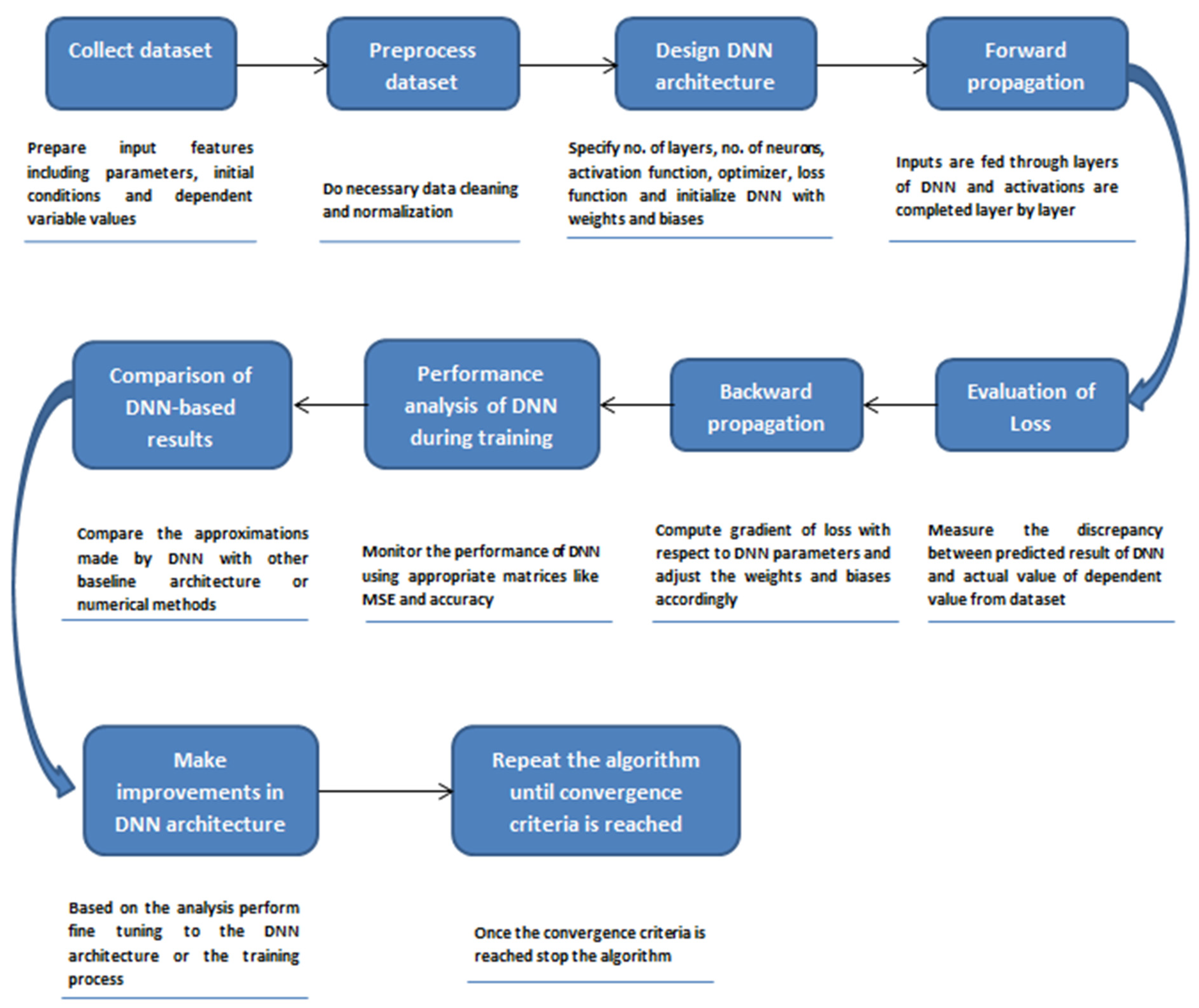
The theories of nonlinear dynamics, or “the study of complexity,” offer a strict, mathematical foundation for the description of living things. Consequently, both nonlinear dynamicists and biologists need to be knowledgeable about nonlinear dynamics. We considered the Sel’kov model in order to apply our proposed DNN-based approach to the simulation of nonlinear dynamics. Two nonlinear differential equations are used in the model to characterize the amounts of the two chemical species that are engaged in glycolysis. Its simplified version of temporal dynamics in mathematical form is given as follows:

$$\left\{\begin{array}{c}\frac{du}{dt}=-u+av+u^{2}v \left(a\right)\\ \frac{dv}{dt}=b-av-u^{2}v \left(b\right)\\ u\left(0\right)=1, v\left(0\right)=0 \end{array}\right\}$$

(1)

With the inclusion of both positive and negative feedback mechanisms, the Equation (1) reflects the dynamics of the two variables u and v over time.

The dependent variables u and v represent concentrations of adenosine diphosphate (ADP) [22] and fructose 6-phosphate (F6P) [23] in the process of glycolysis. Equation (1)(a) represents the rate of change in the concentration of ADP with respect to time. The term $-u$ indicates the decay of ADP, $a$ ($a>0$) is the rate of the constant for the production of F6P, the term $av$ with a positive sign is responsible for the rate of production of ADP due to presence of $v$ scaled by using parameter $a$, and $u^{2}v$ is responsible for nonlinearity, implying that the concentration of $u$ promotes its own production multiplied by the concentration of $v$.

Equation (1)(b) represents the rate of change in the concentration of fructose 6-phosphate. The term $b$ ($b>0$) is the rate constant for the decay of ADP and the term $-av$ is responsible for the rate of consumption of F6P due to the reaction of $u$ and $v$. The product term $u^{2}v$ indicates nonlinear interactions between two chemical species, suggesting that the concentration of $u$ inhibits the production of $v$. Due to the squared components involving $u^{2}v$, the model shows nonlinearity, which can result in fascinating behaviors such as oscillations or the establishment of persistent steady states.

3. Methodology

For the simulation of the aforementioned problem, we took advantage of a DNN-based strategy to solve a set of nonlinear differential equations. The working rule that DNN follows to solve differential equations is that it codifies the differential equation [24] as a loss function [25,26] for optimization problems and then curtails the loss by adopting different optimization techniques. Here, a thorough explanation of how neural networks function and perform is offered.

3.1. Data Preparation

In approximating a dependent variable of a differential equation using DNN, the type of data typically consists of input features and corresponding dependent variable values. The parameters a and b in our system of differential equations serve as the input features. By input features, we mean the variables or parameters that are known in the situation at hand. We must select definite $a$ and $b$ values as well as the time period at which we wish to approximate. The dependent variable values $u\left(t\right)$ and $v\left(t\right)$ are the solutions of a given system of differential equations at a different time t; these are unknown and must be approximated by DNN. Pairs of input characteristics ($a$, $b$) with their associated values of ($u\left(t\right)$, $v(t$)) at various time points t would make up the dataset.

The fully connected layer can estimate the dependent variable for new input configurations by utilizing this dataset to understand the underlying patterns and connections between the input characteristics and the dependent variable values. The dataset is divided into a training set and a testing set as per the setup of the Python package known as NeuroDiffEq [27].

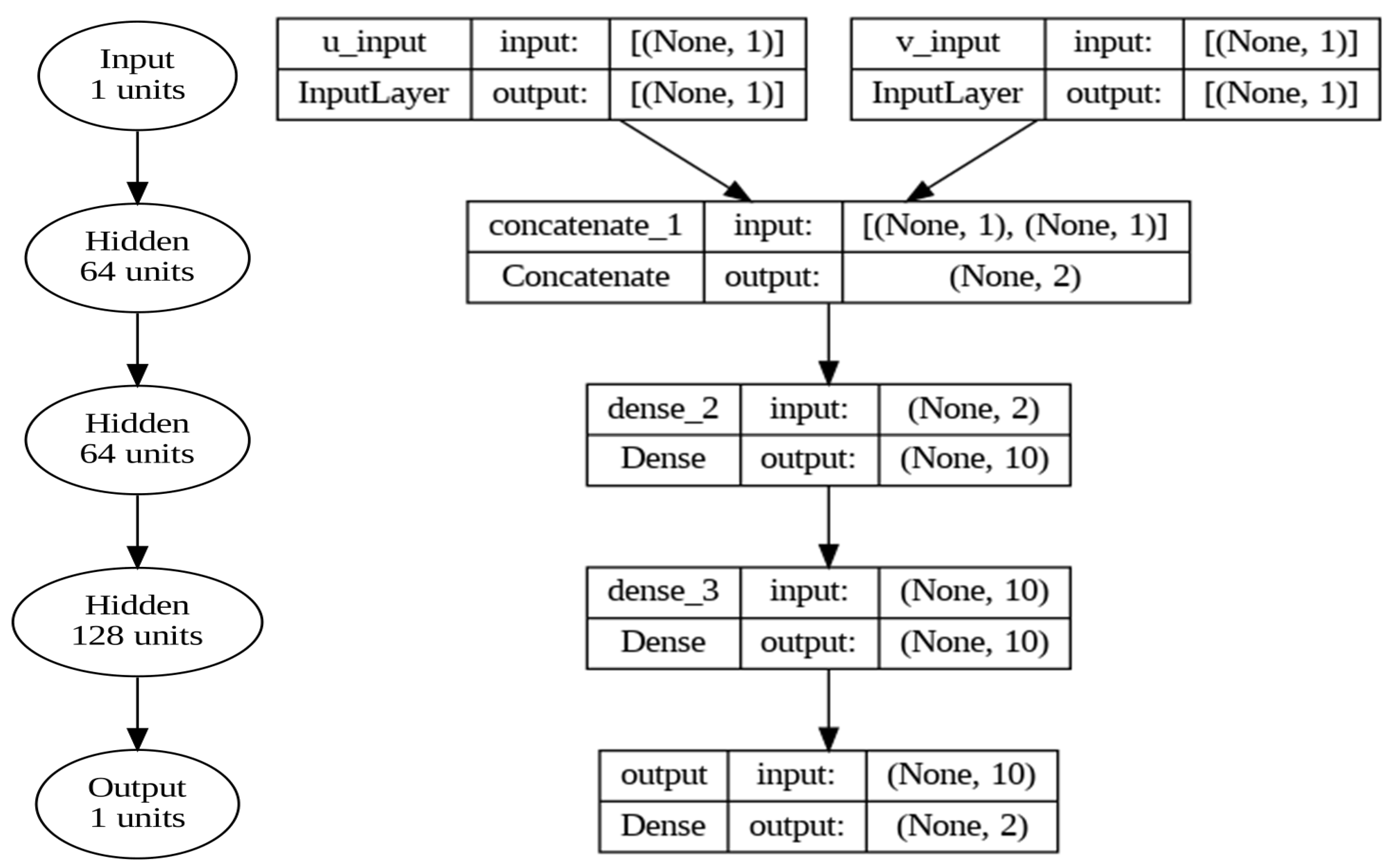
3.2. Neural Network Architecture Design

As baseline architecture, we adopted a fully connected neural network (FCNN) to meet our task described in our proposed methodology.

For each dependent variable, the settings in our model that make the neural network architecture consist of one input layer, one output layer, and three fully connected hidden layers. The first two hidden layers each contain 64 units of neurons, and the third layer has 128 neurons. Before moving on to the next layer, the input is stimulated during the process by using an activation function. The activation function [28], which is in charge of activating neurons, aims to create nonlinearity between the levels. The activation function used in our setup, the Tanh function activation [29], is smooth and continuous. This characteristic of the Tanh activation function enables the network to have continuous and differentiable outputs, supporting gradient-based optimization techniques such as backpropagation. In this baseline architecture of DNN, we adjusted the hyperparameters including the learning rate, activation function, optimization technique, number of layers, and number of neurons per layer manually in the process of training a neural network. Figure 1 and Figure 2 unveil the inner working of the neural network intended for use in the simulation of a given problem. There are several layers in the network, including input, hidden, and output layers, which are connected by weighted connections. To approximate the behavior of the glycolysis system, each layer carries out specialized computations.

3.3. Training of the Model

The model is trained by initializing random weights and biases after all structural settings have been completed. For the training loop, we set epochs to 30,000 and the learning rate to 0.01. The input data are sent forward over the network. After computing the weighted sum of the inputs in each layer, the activation function is applied and the output is propagated to the next layer. A specified threshold value is used by the activation function to determine whether or not a neuron should be stimulated to transfer output to the next layer. This loop keeps running until the output layer is reached. The activation function enhances the expressive power of the fully connected layer. Through this predicted output, the error or the loss is calculated using the appropriate loss function.

Mean squared error (MSE) [30], which is frequently used as a metric for regression problems [31], is adopted here to calculate the average difference between predicted and actual output values in order to measure the performance of the model during training. The mathematical form of MSE is given in Equation (2).

$$MSE=\frac{1}{n}\left({\displaystyle \sum }_{i=1}^n{\left(y_i\_true-y_i\_predicted\right)}^2\right)$$

(2)

• n = the number of sample points in the dataset,
• $y_i\_true$ = true values of the $i^{th}$ sample
• $y_i\_predicted$= predicted values of the $i^{th}$ sample

Using optimization techniques [32] in backpropagation [33], this loss is then minimized to update the model’s parameters (weights and biases) and improve accuracy. The optimization technique we utilized is the integration of momentum and adaptive learning rate techniques; that is, the Adam (adaptive moment estimation) algorithm [34]. It is efficient because even with large datasets, it tends to converge rapidly. The working rule of the Adam algorithm can be summarized mathematically as follows:

$$\left\{\begin{array}{c}{m}_t={\beta }_1{m}_{t-1}+\left(1-{\beta }_1\right){\left(g_t\right)}^2\\ V_t=\sqrt{{\beta }_2{V}_{t-1}+\left(1-{\beta }_2\right){\left(g_t\right)}^2 }\\ {\theta }_{t+1}=m_t-\eta \frac{\sqrt{\left(1-{\beta }_2\right)}}{\left(1-{\beta }_1\right)}.\frac{m_t}{V_{t+ϵ}}\end{array}\right\}$$

(3)

The term $m_t$ is the first-moment estimate and is the mean of the gradients calculated at each time step t, ${\beta }_1$ and ${\beta }_2$ are exponential decaying parameters, $V_t$ is the second-moment estimate which is the variance of the gradients calculated at each time step, $g_t$ is the gradient calculated at each time step t, $\eta$ is the learning rate for regulating the step size in the parameter update, and ${\theta }_{t+1}$ is the updated parametric value at time $t+1$.

3.4. Analysis of the Model’s Performance

Once the model is trained, we validated the model, which helps to improve the performance of the model by adjusting parameters [35] and hyperparameters such as the number of epochs and the learning rate, and then we test the model to see if it could handle new data points. As a final stage, the accuracy and loss of the suggested methodology were determined by comparing the findings to those of a conventional numerical method. We took advantage of the state-of-the-art programming language Python to simulate and visualize the results of our model of a system of a differential equation. The DNN-based technique is clearly illustrated in Figure 3, which makes it easier to analyze and comprehend the steps required in approximating a dependent variable with a DNN.

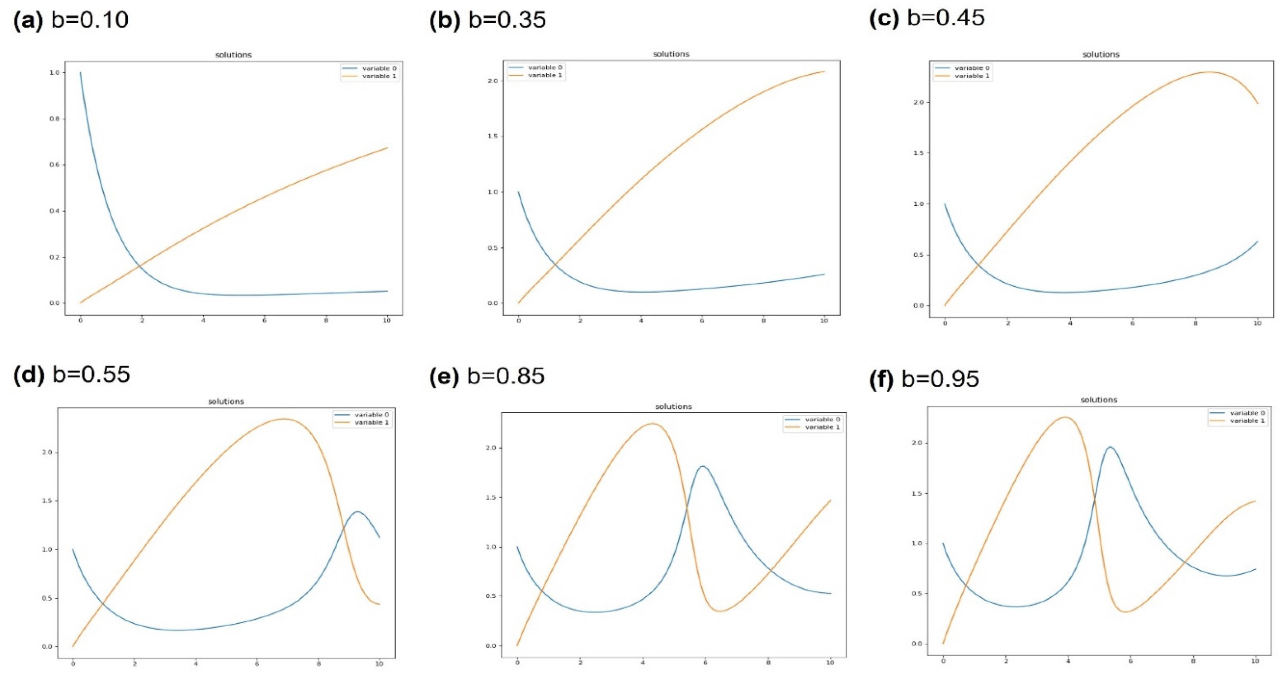
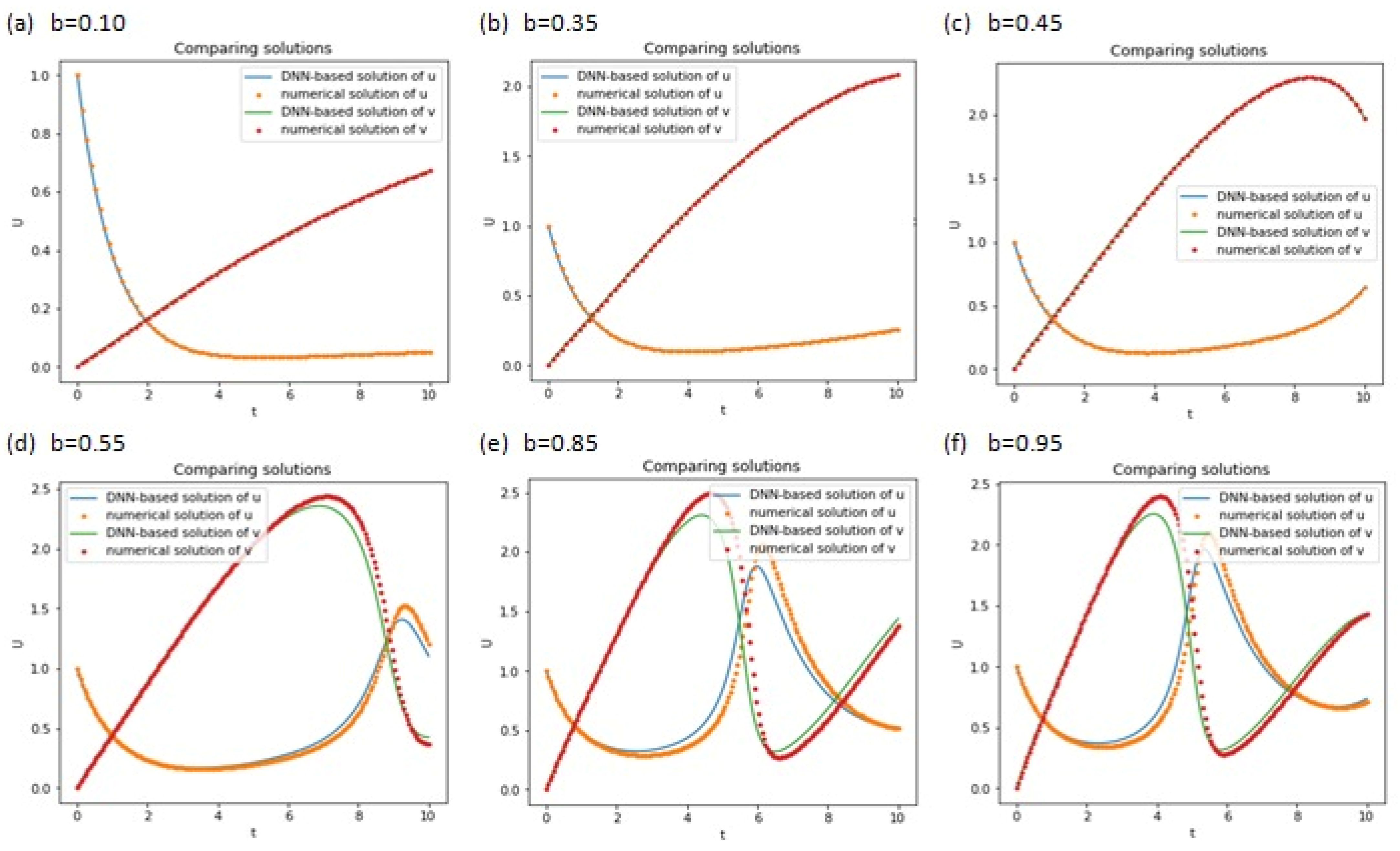
4. Results and Discussion

This section will discuss the simulation results achieved using the suggested DNN-centered scheme. We carried out various experiments to observe how changes in the parametric values of the nonlinear temporal dynamical model provided in Equation (1) can affect the solution of a set of differential equations.

Figure 4 shows oscillations produced during the glycolysis process evaluated using a DNN-based method. We noticed impacts of various values of parameter “b” ranging from 0.10 to 0.95 on the oscillations while holding the parameter “a” fixed to a value of 0.08 as shown in all the graphs of Figure 4. In the second training run, these outcomes were attained. In Figure 4, the orange color represents the solution of Equation (1)(a) and the blue color represents the solution of Equation (1)(b). Figure 4 shows that as the value of “b” rises, there are a growing number of oscillations. For smaller values of b, the oscillations begin as tiny and the graphs for v show monotonic declines while graphs for u show abrupt increases that eventually achieve their maximum value. Oscillation values rise along with increasing values of b, and they abruptly shift after a while.

A comparison between the DNN-based solutions and the solutions obtained from the numerical method (the Runge–Kutta method) are plotted in Figure 5. It is obvious from the graphical results how beautifully the neural network approximated the solution of the nonlinear dynamical system presented in Equation (1). Figure 5 shows plots with dotted lines for neural network approximation and solid lines for numerical method approximation that are very well matched with one another. Runge–Kutta and other numerical techniques can be computationally costly, especially for complicated systems or large-scale problems. Moreover, the cost of computation rises as more iterations are needed to reach a solution. DNN-based solutions can offer predictions or answers significantly faster than numerical approaches once they have been trained. The Runge–Kutta method is predicated on the assumptions and the underlying mathematical model; on the other hand, a DNN can potentially generalize to a wider range of problems once trained on diverse and representative data.

We performed an error analysis and documented the loss and accuracy of the desired model in order to verify the veracity of our suggested advanced DNN-based scheme, as is evident from the bar graph shown in Figure 6. It shows the loss and accuracy for both u and v. It is clear that, starting at b = 0.95, we have little loss but high accuracy, and that, for b = 0.85, accuracy temporarily decreases. However, for a decrease in the value of parameter b, we observed maximum accuracy in the case of b = 0.10. It is observed that the proposed architecture of the DNN outperformed the traditional numerical techniques for the nonlinear dynamical system, as it produces findings that are precise and effective.

5. Conclusions

In conclusion, the proposed DNN-based strategy has proven to be a powerful tool for simulating the Sel’kov glycolysis model, which is a complex nonlinear dynamical system. Through a series of experiments, we have demonstrated that the DNN architecture is effective in capturing the system’s nonlinear dynamics and bifurcation behavior, even when parametric values are changed. In an error analysis, it is helpful to visualize the effects of each parametric value on the dependent variable. The deviance and trends that the model identified are highlighted in the graphical findings. These findings suggest that the DNN-based approach can provide a valuable means for understanding and analyzing the concentration profiles of biochemical reactions. We are confident that our research will contribute to the development of more advanced and effective approaches to solving nonlinear dynamical systems, paving the way for new discoveries in this field. Overall, this study highlights the immense potential of the DNN-based approach in understanding complex systems and advancing scientific research. The proposed strategy can be integrated with recently proposed activation functions to optimize and better capture the complexities of nonlinear dynamical systems. Additionally, extending the proposed methodology to more complex biological models beyond Sel’kov and incorporating the oscillatory activation function [27,36] can offer new opportunities to investigate chemical reactions with vibratory structures.

References

1. El-Safty, A.; Tolba, M.F.; Said, L.A.; Madian, A.H.; Radwan, A.G. A study of the nonlinear dynamics of human behavior and its digital hardware implementation. J. Adv. Res. 2020, 25, 111–123. [Google Scholar] [CrossRef]
2. Peters, W.S.; Belenky, V.; Spyrou, K.J. Spyrou. Regulatory use of nonlinear dynamics: An overview. In Contemporary Ideas on Ship Stability; Elsevier: Amsterdam, The Netherlands, 2023; pp. 113–127. [Google Scholar]
3. Mahdy, A.M.S. A numerical method for solving the nonlinear equations of Emden-Fowler models. J. Ocean. Eng. Sci. 2022, in press. [CrossRef]
4. Yeongjun, L.; Lee, T.-W. Organic synapses for neuromorphic electronics: From brain-inspired computing to sensorimotor nervetronics. Acc. Chem. Res. 2019, 52, 964–974. [Google Scholar]
5. Adina, T.M.-T.; Shortland, P. The Nervous System, E-Book: Systems of the Body Series; Elsevier Health Sciences: Amsterdam, The Netherlands, 2022. [Google Scholar]
6. Money, S.; Aiyer, R. Musculoskeletal system. Adv. Anesth. Rev. 2023, 341, 152. [Google Scholar] [CrossRef]
7. Morris, J.L.; Nilsson, S. The circulatory system. In Comparative Physiology and Evolution of the Autonomic Nervous System; Routledge: London, UK, 2021; pp. 193–246. [Google Scholar]
8. Lakrisenko, P.; Stapor, P.; Grein, S.; Paszkowski; Pathirana, D.; Fröhlich, F.; Lines, G.T.; Weindl, D.; Hasenauer, J. Efficient computation of adjoint sensitivities at steady-state in ODE models of biochemical reaction networks. PLOS Comput. Biol. 2023, 19, e1010783. [Google Scholar] [CrossRef]
9. Fu, Z.; Xi, S. The effects of heavy metals on human metabolism. Toxicol. Mech. Methods 2020, 30, 167–176. [Google Scholar] [CrossRef]
10. Wu, G. Nutrition and metabolism: Foundations for animal growth, development, reproduction, and health. In Recent Advances in Animal Nutrition and Metabolism; Springer: Berlin/Heidelberg, Germany, 2022; pp. 1–24. [Google Scholar]
11. Basu, A.; Bhattacharjee, J.K. When Hopf meets saddle: Bifurcations in the diffusive Selkov model for glycolysis. Nonlinear Dyn. 2023, 111, 3781–3795. [Google Scholar] [CrossRef]
12. Dhatt, S.; Chaudhury, P. Study of oscillatory dynamics in a Selkov glycolytic model using sensitivity analysis. Indian J. Phys. 2022, 96, 1649–1654. [Google Scholar] [CrossRef]
13. Pankratov, A.; Bashkirtseva, I. Stochastic effects in pattern generation processes for the Selkov glycolytic model with diffusion. AIP Conf. Proceeding 2022, 2466, 090018. [Google Scholar]
14. Montavon, G.; Samek, W.; Müller, K.-R. Methods for interpreting and understanding deep neural networks. Digit. Signal Process. 2018, 73, 1–15. [Google Scholar] [CrossRef]
15. Ul Rahman, J.; Faiza, M.; Akhtar, A.; Sana, D. Mathematical modeling and simulation of biophysics systems using neural network. Int. J. Mod. Phys. B 2023, 2450066. [Google Scholar] [CrossRef]
16. Rehman, S.; Akhtar, H.; Ul Rahman, J.; Naveed, A.; Taj, M. Modified Laplace based variational iteration method for the mechanical vibrations and its applications. Acta Mech. Autom. 2022, 16, 98–102. [Google Scholar] [CrossRef]
17. Zarnan, J.A.; Hameed, W.M.; Kanbar, A.B. New Numerical Approach for Solution of Nonlinear Differential Equations. J. Hunan Univ. Nat. Sci. 2022, 49, 163–170. [Google Scholar] [CrossRef]
18. Kremsner, S.; Steinicke, A.; Szölgyenyi, M. A deep neural network algorithm for semilinear elliptic PDEs with applications in insurance mathematics. Risks 2020, 8, 136. [Google Scholar] [CrossRef]
19. Li, Y.; Wei, H.; Han, Z.; Huang, J.; Wang, W. Deep learning-based safety helmet detection in engineering management based on convolutional neural networks. Adv. Civ. Eng. 2020, 2020, 9703560. [Google Scholar] [CrossRef]
20. Sahu, A.; Rana, K.P.S.; Kumar, V. An application of deep dual convolutional neural network for enhanced medical image denoising. Med. Biol. Eng. Comput. 2023, 61, 991–1004. [Google Scholar] [CrossRef] [PubMed]
21. Pan, G.; Zhang, P.; Chen, A.; Deng, Y.; Zhang, Z.; Lu, H.; Zhu, A.; Zhou, C.; Wu, Y.; Li, S. Aerobic glycolysis in colon cancer is repressed by naringin via the HIF1A pathway. J. Zhejiang Univ. Sci. B 2023, 24, 221–231. [Google Scholar] [CrossRef] [PubMed]
22. Chen, X.; Ji, Y.; Zhao, W.; Niu, H.; Yang, X.; Jiang, X.; Zhang, Y.; Lei, J.; Yang, H.; Chen, R.; et al. Fructose-6-phosphate-2-kinase/fructose-2, 6-bisphosphatase regulates energy metabolism and synthesis of storage products in developing rice endosperm. Plant Sci. 2023, 326, 111503. [Google Scholar] [CrossRef]
23. Hsu, S.-B.; Chen, K.-C. Ordinary Differential Equations with Applications; World Scientific: Singapore, 2022; Volume 23. [Google Scholar]
24. Tian, Y.; Su, D.; Lauria, S.; Liu, X. Recent advances on loss functions in deep learning for computer vision. Neurocomputing 2022, 497, 129–158. [Google Scholar] [CrossRef]
25. Ul Rahman, J.; Ali, A.; Ur Rehman, M.; Kazmi, R. A unit softmax with Laplacian smoothing stochastic gradient descent for deep convolutional neural networks. In Proceedings of the Intelligent Technologies and Applications: Second International Conference, INTAP 2019, Bahawalpur, Pakistan, 6–8 November 2019; Springer: Singapore, 2020. Revised Selected Papers 2. [Google Scholar]
26. Chen, F.; Sondak, D.; Protopapas, P.; Mattheakis, M.; Liu, S.; Agarwal, D.; Di Giovanni, M. Neurodiffeq: A python package for solving differential equations with neural networks. J. Open Source Softw. 2020, 5, 1931. [Google Scholar] [CrossRef]
27. Rahman, J.; Ul, F.M.; Dianchen Lu, D. Amplifying Sine Unit: An Oscillatory Activation Function for Deep Neural Networks to Recover Nonlinear Oscillations Efficiently. arXiv, 2023; arXiv:2304.09759. [Google Scholar]
28. Roy, S.K.; Manna, S.; Dubey, S.R.; Chaudhuri, B.B. LiSHT: Non-parametric linearly scaled hyperbolic tangent activation function for neural networks. In International Conference on Computer Vision and Image Processing, Nagpur, India, 4–6 November 2022; Springer Nature: Cham, Switzerland, 2022. [Google Scholar]
29. Qi, J.; Du, J.; Siniscalchi, S.M.; Ma, X.; Lee, C.-H. On mean absolute error for deep neural network based vector-to-vector regression. IEEE Signal Process. Lett. 2020, 27, 1485–1489. [Google Scholar] [CrossRef]
30. Tianle, C.; Gao, R.; Hou, J.; Chen, S.; Wang, D.; He, D. A gram-gauss-newton method learning overparameterized deep neural networks for regression problems. arXiv 2019, arXiv:1905.11675. [Google Scholar]
31. Yong, H.; Huang, J.; Hua, X.; Zhang, L. Gradient centralization: A new optimization technique for deep neural networks. In Proceedings of the Computer Vision–ECCV 2020: 16th European Conference, Glasgow, UK, 23–28 August 2020; Springer International Publishing: Cham, Switzerland, 2020. Proceedings, Part I 16. [Google Scholar]
32. Wright, L.G.; Onodera, T.; Stein, M.M.; Wang, T.; Schachter, D.T.; Hu, Z.; McMahon, P.L. Deep physical neural networks trained with backpropagation. Nature 2022, 601, 549–555. [Google Scholar] [CrossRef] [PubMed]
33. Ariff, N.A.M.; Ismail, A.R. Study of adam and adamax optimizers on alexnet architecture for voice biometric authentication system. In Proceedings of the 2023 17th International Conference on Ubiquitous Information Management and Communication (IMCOM), Seoul, Republic of Korea, 3–5 January 2023; IEEE: Piscataway, NJ, USA, 2023. [Google Scholar]
34. Legaard, C.M.; Schranz, T.; Schweiger, G.; Drgoňa, J.; Falay, B.; Gomes, C.; Iosifidis, A.; Abkar, M.; Larsen, P.G. Constructing Neural Network Based Models for Simulating Dynamical Systems. ACM Comput. Surv. 2023, 55, 236. [Google Scholar] [CrossRef]
35. Hong, Z.; Lu, Y.; Liu, B.; Ran, C.; Lei, X.; Wang, M.; Wu, S.; Yang, Y.; Wu, H. Glycolysis, a new mechanism of oleuropein against liver tumor. Phytomedicine 2023, 114, 154770. [Google Scholar] [CrossRef] [PubMed]
36. Jamshaid Ul, R.; Makhdoom, F.; Lu, D. ASU-CNN: An Efficient Deep Architecture for Image Classification and Feature Visualizations. arXiv 2023, arXiv:2305.19146. [Google Scholar]
Figure 1. The figure visually encapsulates the in-depth exploration, unveiling the intricate inner workings of neural networks.
Mathematics 11 03216 g001
Figure 2. The complete neural architecture comprises hidden layers 1, 2, and 3, consisting of 64, 64, and 128 units respectively.
Mathematics 11 03216 g002
Figure 3. Description for the DNN-based model for the simulation of a nonlinear dynamical system.
Mathematics 11 03216 g003
Figure 4. Representing the solutions of the Sel’kov glycolysis model for different values of kinetic parameters using a DNN-based approach.
Mathematics 11 03216 g004
Figure 5. A comparison of DNN-based solutions and numerical solutions of the Sel’kov glycolysis model with different kinetic parameters.
Mathematics 11 03216 g005
Figure 6. Error analysis of the Sel’kov glycolysis model with different kinetic parameters.
Mathematics 11 03216 g006
Disclaimer/Publisher’s Note: The statements, opinions and data contained in all publications are solely those of the individual author(s) and contributor(s) and not of MDPI and/or the editor(s). MDPI and/or the editor(s) disclaim responsibility for any injury to people or property resulting from any ideas, methods, instructions or products referred to in the content.