Abstract
Selective laser sintering (SLS) is one of the most popular 3D molding technologies; however, the manufacturing steps of SLS machines are cumbersome, and the most important step is focused on molding testing because it requires a lot of direct labor and material costs. This research establishes advanced hybrid mathematical classification models, including random forest (RF), support vector machine (SVM), and artificial neural network (ANN), for effectively identifying the SLS yield of the sintering results from three sintered objects (boxes, cylinders, and flats) to achieve the key purpose of reducing the number of model verification and machine parameter adjustments, thereby saving a lot of manufacturing time and costs. In the experimental process, performance evaluation indicators, such as classification accuracy (CA), area under the ROC curve (AUC), and F1-score, are used to measure the proposed models’ experience with practical industry data. In the experimental results, the ANN gets the highest 0.6168 of CA, and it is found that each machine reduces the average sintering time by four hours when compared with the original manufacturing process. Moreover, we employ an oversampling method to expand the sample data to overcome the existing problems of class imbalance in the dataset collected. An important finding is that the RF algorithm is more suitable for predicting the sintering failure of objects, and its average sintering times per machine are 1.7, which is lower than the 1.95 times of ANN and 2.25 times of SVM. Conclusively, this research yields some valuable empirical conclusions and core research findings. In terms of research contributions, the research results can be provided to relevant academic circles and industry requirements for referential use in follow-up studies or industrial applications.
Keywords:
selective laser sintering; random forest; support vector machine; artificial neural network; oversampling method MSC:
03C13; 18B05
1. Introduction
In this section, we introduce why selective laser sintering (SLS) is studied and describe the important problems encountered in the manufacturing process of SLS machines. Then, we illustrate the relevant industrial application research of SLS and machine learning (ML) techniques, and we also explain the purpose of the relevant research.
1.1. Research Problems and Research Motivation
With the progress of the times, ordinary 2D printers can no longer meet customers’ needs for storing memories or data, and even 3D additive manufacturing (3D-AM) can improve people’s quality of life significantly. The inventor of the first 3D molding machine focused on using this excellent device to shorten the time for product design; at that time, it took about 5 to 8 weeks from plastic mold opening to plastic injection for the traditional manufacturing process, but now it could be shortened to several hours through the 3D-AM printing device and we could know instantly whether the product design was successful and available. With the advent of the information technology era, a variety of 3D-AM technologies have surfaced, from the simplest fused deposition modeling (FDM) to stereolithography (SLA), SLS, and finally direct metal laser sintering (DMLS) techniques. These technologies have their own advantages and difficulties; in particular, SLS becomes an excellent technology among them at this stage. The justified reason is that SLS has a variety of materials to choose from, and each material has different characteristics. These characteristics are highly dependent on the sintering temperature, and thus the temperature has become one of the many factors that need to be overcome in the SLS manufacturing process. However, the application use of SLS is very wide, particularly in pharmaceutical manufacturing [1]; there will be different usages according to the properties of different materials [2]. Interestingly, in order to make SLS with more industrial applications, there is even a study [3] that points out the coloring research of extra functions for SLS to increase the multi-application of SLS.
The so-called SLS [4,5] has the function of using laser and Galvo scanning systems (GSS) to draw the outline of objects (e.g., boxes, cylinders, and flats) on specific materials [6], and it is stacked layer by layer; following that, the noodles need to be heated through a heating system and accurately maintained at an appropriate temperature. The temperature setting needs to adjust different temperature values according to the different properties of materials. Based on their different natures, some materials require lower temperatures but have stronger toughness, and some materials require higher temperatures but have stronger hardness. However, there have been some fatal problems for research. First, this technique must build a heating system on the basis of a laser, and the laser system is very sensitive to heat, which may cause the deflection of the GSS meter [7], resulting in dimensional size errors of the molded object and in turn affecting the result of sintering. Second, in the SLS technique, the accuracy of the motor, the scanning accuracy of the laser and GSS, and the size of the laser power will deeply affect the sintering result or sintering quality [8,9]. SLS is melted at high temperatures, which means that it will pollute the natural environment [10], and thus it is an important issue for the difficulty addressed in how to recycle the powder after high temperatures and to measure the strength of sintering after using the recycled powder [11]. These are the SLS industry’s major problems that must be faced at present. From an industrial perspective, if the use of these powder materials cannot be avoided now, reducing unnecessary testing procedures by using an effective binary classification model or technique will be an important issue. An accurate testing process can not only reduce the use of manpower but also reduce the pollution generated during the testing process. Thus, to construct such an effective classification technique motivates and rationalizes this research.
Regarding binary classification models, some techniques from data mining and deep learning [12,13] have been highly and widely used in various industrial application fields with good performance. In particular, further data analysis can be done for the collected industrial data to find more clues, and the importance of advanced models to industrial applications and data analysis is thus, further inspired. Based on the meaningful descriptions mentioned above, this research has the interest of designing advanced binary models to address the data analysis of industry applications. The accelerated triggering of the research is highlighted in developing an effective prediction system for driving the research’s model for identifying manufacturing processes in the SLS industry.
1.2. Relevant Research Purposes
In the research related to 3D printing and deep learning techniques, some of them construct an identification mechanism to detect bed defects in powders through convolutional neural networks (CNN) [14]. In this study, the related data of the sintering process is collected and then put into the training mechanism of the CNN; after this training, it is identified whether the sintered object is formed smoothly and successfully. In the study [15], a semi-supervised learning method is used to predict whether the model is suitable for selective laser melting; the cases collected after actual sintering are thrown into the training network. Different types of data are generated by a generative adversarial network (GAN) to be evaluated due to the difficulty of actual sintering and the high cost of materials, thereby resulting in a small number of experimental samples obtained for the available data. In the study of Stathatos et al. [16], the laser power, speed, or energy during sintering is trained with ML techniques, and then the trajectory and energy of each laser sintering have an active optimization adjustment; finally, verification is performed after all 3D objects are formed. In the study of Shen et al. [17], the energy density of the object is estimated by sintering parameters such as laser intensity, scanning speed, scanning interval, and layer thickness, so that the results of strength and scalability for the sintered object can be predicted by supervised learning methods.
Through the above descriptions, this research takes the finished product from the SLS machine as the research object and provides a comparison of the difference between the old and new SLS production processes by analyzing the characteristic data for process improvement. Thus, this research is based on the hybrid mathematical models [18,19] with the following research purposes: (1) The research proposes a hybrid mathematical binary classification model, including random forest (RF) [20], support vector machine (SVM) [21], and artificial neural network (ANN) [21], due to their past superior performance, combined with an oversampling method for the data used due to the problem of class imbalance. (2) The method of cross-validation and the evaluation index of these algorithms are used for the industry data application of identifying SLS production processes. (3) By the predictive model, the sintering results are obtained in advance before the actual sintering, and the machine parameters are adjusted in advance for the SLS equipment; it is a key point that the actual sintering is not performed until it is predicted to be successful. (4) With this research, the number of sintering times, the number of adjustments during sintering, and the time and cost spent verifying the machine are reduced. (5) This research provides an applicable contribution with practical industry value.
The structure of this research is divided into six sections, as follows: The Section 1 is the introduction, which explores the research background and the prior industry applications as the research base. The Section 2 is the technical background applications, including reviews of the SLS techniques, the three well-known classification algorithms, the cross-validation method, and the evaluation standard. The Section 3 is the step-by-step algorithm of the hybrid mathematical binary classification model constructed in this research. The content focuses on the introduction of the experimental process and explains how to obtain data, build models, use an oversampling method, and compare sintering and adjustment times. The Section 4 is the empirical results of the effectiveness analysis and evaluation measurement after the demonstration; the Section 5 addresses research findings and research limitations. Finally, the Section 6 is about the study’s contribution and future prospects.
2. Related Technical Works
This section reviews and explores the relevant technical background of identifying SLS, three classification algorithms, the cross-validation method, and evaluation indicators.
2.1. SLS Technology with Its Applications
The SLS [22] is to use a laser to select the area to be formed, while the unformed area should be in powder form. For the SLS applications, some core features (factors) have been determined. If the temperature [23] controlled by the heater is too high, the unsintered area agglomerates, and this increases the difficulty of picking up items. If the temperature is controlled too low, the temperature of the area to be formed is pulled due to the contrast with the air temperature in the sintering chamber, causing the object to bend; in a slight case, the size of the formed object is inconsistent and wrong, and in a serious case, the object is unable to form [24]. However, if during the sintering process of an object [25], high temperatures and low temperatures appear alternately, or even if the temperature distribution is uneven during the sintering process on the same plane, it causes some problems, such as insufficient strength of the object, inaccurate size of the object, and even failure to form the object. Thus, the layout and control of the heater are very important. Furthermore, each material has a different temperature range. Some materials have a high temperature and a small operating range, but they have high strength after molding; conversely, some materials have a low temperature and a large operating range, but they have strong toughness after molding. Under such circumstances, it becomes a very important issue to ensure that each material can be controlled within the range of its properties [26]. In summary, it is better that the smaller the temperature change, the smaller the range of temperature distribution [27]. Except for the above influences, it is also a factor that the laser is not powerful enough to penetrate the powder, which causes sintering defects. Importantly, there are three research directions defined. (1) The energy definitely affects the shape of the object, so we can use the instrument to collect the intensity of the laser energy as a very useful feature, which is used to dig out the relationship between the laser energy and the sintering result. (2) Another factor that affects the sintering result is the spot size of the laser. When the spot size is larger and the path overlap is higher, the energy density is stronger and the sintering speed is faster. Conversely, the smaller the spot size, the more compact the path is planned, so the sintering speed is slower but the sintered objects are finer. Thus, we identify the spot size as one of the features to predict the sintering result. (3) The galvanometer system often has pin distortion and barrel distortion, which affect the size of a single plane of the object, and the error of the single size is continuously amplified throughout the sintering process, which causes dimensional (size) errors of the overall object. Thus, we also collect the error amount as a feature to judge the sintering result.
For the manufacturing process of SLS [28,29], two key processes are identified. First, the target temperature must be set at the beginning of the process, and the temperature of the sintering chamber is raised and stably controlled at the target temperature through the controller to control the heater; this process is called preheating. Second, accordingly, wait for the temperature to reach a certain point and then start sintering. During the sintering process, powder needs to be supplied to the powder surface structure, and then reheating and laser scanning are performed; this process is called sintering. After the graphics on each layer hit the powder surface through the laser, the temperature needs to be lowered. Since the difference between the sintering temperature and the room temperature is too large, if it is taken out directly, the object is directly cooled and deformed, so it takes a long time for natural cooling to cool it. Figure 1 shows the entire SLS process flow. By sintering these objects, it is possible to know whether the molding is successful or not. Thus, we use the following three directions to identify it: (1) Measure the size of the sintered cube; the horizontal (X) axis and the vertical (Y) axis are both 30 mm ± 0.3 mm, and it is a sintered benchmark for success within this size range. (2) Observe whether the lines are completely connected and whether the lines are broken. If there is no break, the test is passed. (3) Observe the sintered gap. If the gap cannot be clearly seen, it means that the details of the gap cannot be clearly displayed, which means that the sintering has failed.
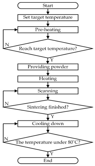
Figure 1.
Sintering process flow of SLS.
With the above sintering process and application of SLS [30,31], it is clear that SLS is a specific technology that requires long-term, precise control to complete. If the number of sintering times is reduced in the verification process, the verification cost is greatly reduced. We collect the sintering data as featured attributes for training to judge the sintering results, and we conduct a repair process on samples that have failed sintering.
2.2. Classification Algorithms
This section reviews the three mathematical classification algorithm models: RF, SVM, and ANN for supervised training to predict the SLS result, respectively.
2.2.1. Random Forest
In the field of classification applications, RF belongs to the Bagging training method. The Bagging concept is to randomly select training samples from the training data and put them back after selection, which means that there is a chance to draw out the same sample again next time, and even the selection of features during growth is random. This training method determines the diversity of the RF, and the combined results are more accurate. After the features are selected, a decision tree is built one by one, and finally, after a series of feature selection (FS) and tree growth, the result is a lot of trees, which are the so-called RFs model. RF is a combination of multiple decision trees, but there is no connection between different decision trees; decision trees determine the correct features by choosing the degree of disorder or entropy and determine the direction of tree growth, and the complexity or entropy must converge to grow. Every time a node is passed, it is in the messiest state at the beginning, and the messiness gets smaller and smaller. Importantly, RF can solve the overfitting problem that other classification methods have [32]. The overfitting problem is to closely match a specific data set so that it cannot be well adapted to other data, resulting in the original correct result being classified in the wrong category. If the RF wants to avoid overfitting, it needs to meet two conditions: one is that the trunk of the tree must be larger and must reflect the law of the big tree, and the other is that the randomness must be sufficient. Otherwise, if the sampling is biased towards a certain feature, trees of different properties cannot be obtained, and an overfitting problem occurs.
Moreover, due to the wide range of industrial applications for RF classifiers, some researchers had used RFs to predict real-life problems faced in different fields, such as the analysis of the surface roughness and mechanical properties of 316L samples produced by SLS [18], the ML prediction of SLS-AM part density [33], and the prediction for the 3D printability of SLS formulations [34]. In the study of Jaime et al. [35], the user is guided to choose which classification method is more suitable for different types of data sets, and how many samples do a RF need? Interestingly, the research results of Oshiro et al. [36] just illustrated and verified this application issue. In the study of Peng et al. [37], various types of in situ monitoring and defect detection methods (e.g., RFs) and their applications are reviewed for the SLS processes.
This research chooses RF as one of the training algorithms first based on the fact that it can avoid overfitting problems. The second reasonable reason is that there is not enough training data, and RF can process it with good performance. It is evidence that the characteristics of multiple trees for RFs can be established through the “big tree rule” to strengthen the training data.
2.2.2. Support Vector Machine
SVM is a very popular classification method with a wide range of applications. SVM can be used to detect network attack traffic [38]; particularly, the enhanced SVM method is used to classify porosity defects during the SLS process [39]. SVM is a supervised learning method based on the linear classification method; it can add support vectors to increase the tolerance of misclassification, and it adds kernel functions to solve nonlinear classification problems that linear classification methods cannot solve. SVMs have a place in ML by virtue of their ability to calculate linearly separable dichotomies, solve linearly inseparable kernel functions, and develop robust and rigorous mathematical theories. The importance and process of SVM are highlighted as follows:
- (1)
- SVM is mainly divided into two types of hard cutting and soft cutting. Although both methods hope that the farther the boundary distance between them is the better, hard cutting does not allow other support vectors to appear between the support vectors, which will easily cause the problem of overfitting.
- (2)
- When encountering linear inseparability, it is necessary to increase the dimension by one level through the kernel function; thus, the two-dimensional feature space is mapped into a three-dimensional feature space through the kernel function, then the support vector is found, and further, the hyperplane is found for processing the classification of features. So far, many calculation methods for kernel function algorithms have been announced, such as linear kernel function, polynomial kernel function, and Gaussian kernel function, which are studied and explored, and each kernel function has its corresponding parameters and suitable application occasions.
- (3)
- We know that when all data is mixed together, it is impossible to distinguish them in a straight line from the perspective of a real-life situation. Accordingly, the SVM maps the feature space from the original dimension to a higher-dimensional feature space through the kernel function, and after mapping to a higher-dimensional space, we use different angles to observe the distribution of each feature [40].
Since SLS is a nonlinear system, this research expects to predict the yield of SLS by using the characteristics of SVM and kernel function to obtain good classification results, and the use of SVM is based on its past outstanding performance.
2.2.3. Artificial Neural Network
A neural network is an algorithm developed by simulating the nerves of a living being. With the advancement of the times, research on various types of ANNs has begun to grow exponentially; ANN has become synonymous with artificial intelligence. The application examples and uses of ANNs have been quite extensive, such as using ANNs to model solar energy systems [41], using ANNs to solve second-order boundary value problems [42], illustrating the recent application of ANNs in the study of Oludare et al. [43], and re-examining the similarity of ANN representations in the study of Kornblith et al. [44]. In particular, Stathatos and Vosniakos used ANNs for arbitrary long tracks in the laser-based AM of the SLS process [16]. In the related field of studying ANNs, there are many derived ANN models used for specific purposes in industry applications. CNN is used for visual recognition of images; especially, the study of Westphal and Seitz [45] based on CNN and ML methods offers an alternative approach for addressing non-destructive quality assurance and manufacturing files with good performance during part manufacturing of SLS. Yuan et al. [46] also used CNNs to well recognize desired quality metrics from videos in the SLS dataset.
The ANN consists of three routings, including an input layer, a hidden layer, and an output layer, and the connecting line between each layer represents a weight. When the weight is output by the activation function and reaches the threshold, it means that the neuron is activated and the data is transmitted to the next level. As to the activation function, it has many kinds of nonlinear functions, such as sigmoid and tanh, while the linear function has ReLU. From reviewing the literature, most studies confirmed that the linear activation function effectively solved the problems of gradient disappearance and gradient explosion. If we modify the weight value to achieve the effect of learning, backward propagation transfer is an important mechanism. In the process of supervised learning, the system randomly gives each neuron a weight, and the ANN uses these weights to calculate the first output value. However, the output value may be a messy value, in which case we calculate the cost value through the output value. The cost value is the squared difference between the predicted result and the actual result, and the smaller the squared difference, the higher the accuracy rate. In each backward pass, it modifies the weight value between each neuron from the back to the front based on the cost function, then repeatedly executes the output result, calculates the cost value, and passes the back-propagation network until the cost function is close to or equal to 0, and the complete neural model is finished. Figure 2 shows a schematic diagram of backward transmission.
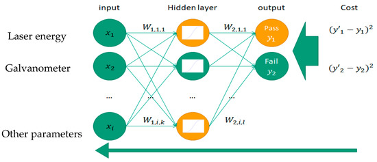
Figure 2.
Schematic diagram of backward propagation transfer.
Due to the power and versatility of the ANN, if we need to modify the model used, it is only necessary to remove or add neurons. This advantage makes the application of the ANN much higher than other algorithms; thus, this research organizes the ANN model to identify SLS results to get good research results with supportability.
2.3. Cross-Validation Method
The commonly used cross-validation methods are quite extensive. We study the reliable accuracy estimation of K-fold cross-validation [47], optimize the cross-validation method and apply it to time series data with the ANN model [48], use genetic algorithm (GA) to optimize the SVM and K-means algorithms plus the K-fold crossover verification method for the mapping of mineral perspectivity [49], and employ ANN, SVM, and RF with hyperparameter tuning by GA optimization for the prediction of landslide susceptibility [50], etc. They are all verified through the cross-validation method to verify real-life issues. There are many effective types of cross-validation, including random example validation, leave-one-out cross validation, test on training data, K-fold cross validation, etc. They have attracted much concern about influencing performance from many researchers.
2.4. Evaluation Indicators of Verification
Evaluation indicators are used for the main function of judging the quality of the classifier. Commonly used indicators include area under ROC (AUC), classification accuracy (CA), F1-score, precision rate (PR), and recall rate (RR) used to measure the classification model for further verification [45,51]. For these indicators, confusion matrix is a core role and very versatile for different application fields, such as a CNN based on ML techniques widely used to classify good and defective image data recorded for AM parts [45], altering a SVM model with the FS method compared to those of the classical soft margin model through the confusion matrix [52], and based on the confusion matrix by different metrics for comparing two SVM models for AM [53]. They are described in detail as follows:
- (1)
- Confusion matrix: it has four different prediction results, including true positive (TP_C), true negative (TN_C), false positive (FP_F), and false negative (FN_F).
- (2)
- CA: the main purpose of the CA rate is to evaluate the performance of the model with a high value, but it cannot distinguish which category is the accuracy rate. Thus, if there is no special requirement for a certain category, we use this indicator to judge the model. The mathematical Formula (1) of the CA rate is formatted as:
- (3)
- PR and RR: it is a key purpose that the PR and RR provide a more accurate analysis of the samples for the binary of success or failure classes, respectively, which is helpful to describe the model for the practical application of product production. The following Formulas (2) and (3) are formatted for the PR and RR, respectively:
- (4)
- F1-score: the F1-score reflects the weight and average of the PR and RR, and it reflects the most balanced value of the PR and RR when neither of them get the best score. The following mathematical Formula (4) of the F1-score is formatted. If the difference between the two values of PR and RR is too large, this value will tend to be smaller.
- (5)
- Receiver operator characteristic (ROC) and AUC: ROC represents the change in decision threshold between the TP_C rate and the FP_F rate. An important purpose of calculating the ROC curve is to derive the AUC value. AUC is a probability, which means that when randomly given a sample of successful cases, the classifier correctly judging the value of a success is higher than judging the value of a failure. The related research on AUC has focused on (1) using AUC to classify the performance of unbalanced data for risk prediction of Chronic Obstructive Pulmonary Disease [54], (2) performance metrics of AUC to identify these intrinsic properties of AM-focused alloy design [55], and (3) using time-dependent AUC to address mortality or readmission prediction for hospitalized heart failure patients [56]. The AUC has three evaluation results: (a) AUC = 1: it represents the perfect classification of the sample data by this classifier; (b) 1 > AUC > 0.5: this represents better than random guessing; and (c) AUC ≤ 0.5: it means that the sample data is not suitable for this classifier.
This research mainly uses the above-mentioned excellent evaluation indicators to evaluate the model built and measure the analytical result after the cross-validation method to determine whether these classifiers are suitable for the SLS production process.
3. Materials and Methods
In this section, the research proposes a model to address the study topic used in materials and methods, and the proposed model has the following four main stages: (1) data collection stage: collect data through corresponding instruments and divide the given data into training data and testing data; (2) model building stage: build a model through training data with a cross-validation method and observe the real results of the validation; (3) oversampling method stage: carry out an oversampling method on the data to establish a classification model again and compare with the model results without processing the oversampling technique; and (4) process improvement stage: through the prediction results of the testing data, compare the sintering times and machine adjustment times of the new and old processes to judge how much labor time is saved. Thus, the proposed model has: data collection ➔ model building ➔ oversampling method ➔ process improvement. Accordingly, the four stages are described in the following four subsections, respectively.
3.1. Data Collection Stage
Data is an important part of AI, and data mining is an important technique of data analysis. It can obtain information related to the target from some irregular data. We introduce the data collection stage by experiencing this research object in the case of the manufacturing process for the SLS industry, and thus the data acquisition and processing flow are divided into the following core data features for defining the data collection:
- (1)
- Core features for data collection are first identified: we first identify the core features, such as the moving amount and inclination degree of the motor on the X and Y axes of the construction platform, the power energy of the laser system at 50%, the spot size of the laser, the scanning error of the galvanometer system, etc. We use the analysis method for the above feature data to predict the success rate of product molding in advance during the manufacturing process. Measure the movement of the vertical motor through the dial gauge. When the platform moves down once, the distance measured by the dial gauge should be 0.1 mm, and this value is recorded as a core feature (factor) to be used as the basis for the classification model.
- (2)
- Collect all data for a successful sintering module when the laser energy is 50%: laser system measurements require specific and expensive instrumentation. We put the light beam into the laser power meter, measured it through the probe, and converted it into an electrical signal. The power meter integrates the read value and the converted value and records the value on the connected computer through a USB port. This value is measured when adjusting the laser galvanometer control system. In the test production phase, since the energy distribution obtained by each laser with the same energy is different, it is tested to see how much power the laser will output when the laser energy is 50%. In the case of simulated maintenance, the measured energy distribution is regarded as a set of modules to simulate the replacement of the laser module, and the successful sintering module is replaced by the sintering failure machine to observe the simulation result after repairing.
- (3)
- Data on spot size is also collected: regarding the spot size of the laser, we use a beam analyzer to measure the size of the laser beam. Each different type of beam analyzer has a different measurement wavelength and energy range. Therefore, we must first know the required laser specifications and then select the correct measuring instrument; otherwise, the instrument itself is damaged. The size of the spot affects the degree of detail when the object is formed. Generally speaking, the smaller the size, the more delicate the object is formed, but the molding time is longer, and vice versa. Importantly, the specification range of the spot size set by the machine is 500 um~600 nm. The scanning error of the galvanometer system brings about information about the error of the plane size. Due to the principle of the galvanometer system, the system has a distortion problem, which affects the horizontal dimension error of the sintered object. However, the method of measuring the error can use the weakest energy to print a dot every one centimeter on the white paper, fill the preset scanning range, and calculate the distance between the dots through image recognition. Then, record the values of the maximum error and the average error.
- (4)
- The type data of boxes, cylinders, and flats and the total result are defined: judge whether the sintering is a successful product by each sintered object, and the basis or key point for judging is to measure whether the sizes of the box meet the specifications, check whether the lines of the cylinder are complete, and whether the gap between the flats is clear. Importantly, when one of the objects is marked as a failure, the total result is marked and classified as a failure; otherwise, it is marked as a pass product. After that, follow-up supervised learning models are used for this data.
- (5)
- All data is collected and used: in this research object, Figure 3 shows the relationship diagram for all the data. In this part, 10 copies of all data are made. In Figure 3, six samples are randomly selected from each of these 10 copies as testing samples, and the rest are used as training data. The training data is used to build a model, and the cross-validation is used to obtain the verification evaluation index after the model is built. The testing data is used to verify the prediction results of the models.
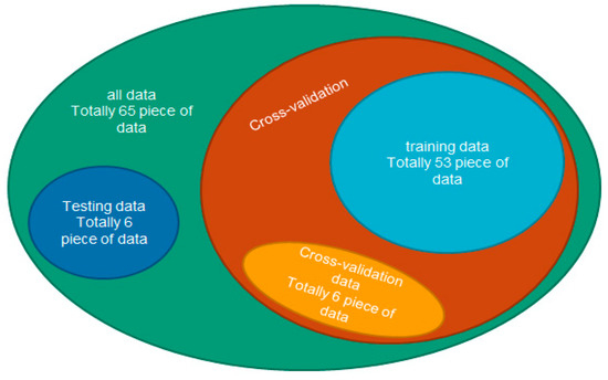 Figure 3. Relationship diagram of research data.
3.2. Model Building Stage
This research uses Orange software to test the data and then verify the predictions. Figure 4 shows the architecture diagram of the proposed model. In Figure 4, we see all the processes and the main components of the prediction model structure. The main components or results are training data (input elements), testing data, oversampling methods, RF, SVM, ANN, cross-validation methods, and prediction results. The operation flow of this model building stage is described in detail as follows: (1) The training data is inputted first, and the form of the parameter is set, which determines whether the role of the value is a feature or the marking result of each sintered object. (2) After these sample data are inputted and transmitted into four components: the cross-validation method, RF, SVM, and ANN. The set of parameters is also passed into the cross-validation method. (3) Take the training data into RF, SVM, and ANN to build a classification model and directly output these three algorithm parameters to the cross-validation method. (4) The cross-validation method is set as a 10-fold, and AUC, CA, and F1-scores are achieved after this calculation of these evaluation indexes is completed in order to preliminarily evaluate the superiority of the classification model.
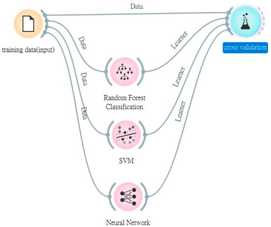
Figure 4.
Architecture diagram of the proposed model with cross-validation method.
3.3. An Oversampling Method Stage
In the data of asymmetric categories (or classes), the CA rate is often high, but there are some unrealistic situations, such as the class imbalance problem (resulting in an illusion of high accuracy rates). To avoid this serious problem, an oversampling method to expand the experimental data is a feasible method for processing and addressing it. Oversampling methods mean expanding the asymmetric data of the minority category to the same amount of data as the majority category, so that the classification model is strengthened and the prediction results are more reliable and feasible.
After implementing this stage for an oversampling method for the expansion, we understand that the experimental data becomes larger, which is conducive to subsequent implementation and good use of the three classifiers of RF, SVM, and ANN to establish a classification model again and use relevant test data for prediction.
3.4. Process Improvement Stage
Accordingly, after achieving the testing results of the previous step, the number of sintering times and the number of adjustments are identified and compared. In this process improvement stage, we have the following three main directions to address:
- (1)
- Original verification process: Figure 5 shows the original verification process before the prediction model is established. In Figure 5, after the machine is assembled, it directly carries out sintering and directly observes the sintering result. If the sintering result is a failure, it is repaired and adjusted directly. After the repair, the above process continues to be repeated until the sintering result is successful. Thus, we find that the minimum number of sintering is to start the sintering process after the machine is assembled, and if the first sintering is successful, the verification is completed promptly. However, if the result of the first sintering is a failure product, it means that the second sintering process is required, and if the second sintering is successful, the verification job is completed in two sintering processes. Interestingly, the main goal of this research is to ensure that the verification is completed after the first sintering, so as to avoid the waste of time and cost of the second sintering.
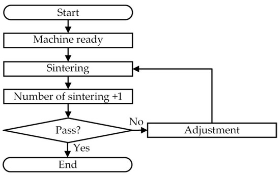 Figure 5. Original verification process.
 - (2)
- Improved verification process: Figure 6 shows the improved process to solve the above problems. The improved verification process is to first pass the prediction results and then decide whether adjustments are required. In Figure 6, after the machine is assembled, the sintering result is predicted first, and the parameters are adjusted when the prediction is a sintering failure. The sintering is performed when the sintering is predicted to be successful. The advantage of this approach is that only the practical sintering failure occurs, in that only the predicted sintering is successful. On the contrary, if it is predicted that the sintering process is a failure, it is adjusted in advance at the time of prediction; thus, the number of sintering times is reduced and the probability of success in the first sintering is increased.
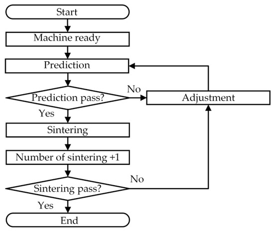 Figure 6. Improved verification process.
 - (3)
- Comparison results before and after process improvement: we use the following methods to count the possible sintering times of the test data: First, we must optimize the original verification process.
- (a)
- Assume that the second sintering is definitely sintered successfully, and there are six test samples in each test data set, of which three are sintered successfully and three are sintered unsuccessfully. Thus, through the original verification process in Figure 5, it is calculated that a total of nine sinterings were required in the original process.
- (b)
- In the new verification process in Figure 6, the rules for defining the number of sintering times are set and presented as follows:
- (i)
- Rule 1: The actual sintering success is also predicted as the sintering success, only needing once sintering;
- (ii)
- Rule 2: The actual sintering failure is also predicted as a sintering failure, only needing sintering once (because the first sintering failure has been predicted in advance);
- (iii)
- Rule 3: The actual sintering is successful, but the predicted sintering is a failure, requiring twice as much sintering;
- (iv)
- Rule 4: The actual sintering failure is predicted to be a sintering success, needing twice as much sintering.
- (c)
- Judge the sintering times according to the above rules, and compare the sintering times of the original process and the improved process. Accordingly, we need to determine the number to adjust the parameters. Figure 7 shows the flow of determining the number of parameters to adjust. When the predicted or actual sintering fails, we perform adjustments according to the process shown in Figure 7. Since no more actual sintering is done, we use some more objective methods to measure it. In practice, for sintered objects, there are probably shapes, such as boxes, cylinders, and flats, that are used to judge the results of sintered objects. The main judgment process is described in the following three directions: First, adjust according to the predicted sintering failure. If it is a box object, in addition to adjusting the error of the galvanometer, it is necessary to adjust the movement of the construction slot motor. Second, when the box object is judged to have failed, two adjustments are required. Third, both cylinder and flat objects only need to be adjusted once and then summed up for each object, which becomes the total number of adjustments in the classification model. The fewer the total number of adjustments, the higher the prediction accuracy.
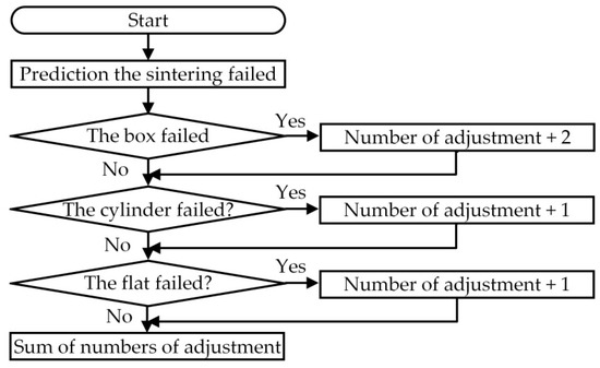 Figure 7. The process of judging the number of parameter adjustments.
4. Empirical Results and Data Analysis Results for a Real Case Study
This section mainly explains the experimental results of random distribution data collected, the cross-validation results of classifiers for each sintered object, the prediction results of classifiers with/without an oversampling method for the given data, and comparison results for the number of sintering and adjustment times for the original verification process and the improved verification process for the purpose of performance evaluation and data analysis. Lastly, the empirical summary from all the experiments and some discussions are further addressed.
4.1. Collection Results of Sample Data
In this section, after the first stage of data collection in Section 3, all 65-sample data with nine features is analyzed, and the detailed information of all samples of feature data is displayed as Appendix A, Table A1. From Appendix A, Table A1, it is found that the box objects have 25 failure cases and 40 successful cases they have 17 failure cases and 48 successful cases for cylinder objects; they have 18 failure cases and 47 successful cases for flat objects; and for total-result objects, they have 37 failure cases and 28 successful cases. Next, Table 1 shows the 10 samples of testing data performed each time with six data points; the testing data is randomly and fairly selected from six of the 65 record samples from the targeted data set each time, and the rest is used for training data. Importantly, it is not guaranteed that the proportion of sintering failure and sintering success for each selected object must be the same.

Table 1.
10 testing samples for each validation with six data.
4.2. Implementing Results of Cross-Validation Method
For the cross-validation results of the case study, we illustrate it with four research objects: box, cylinder, flat, and the total-result into the following four parts, respectively.
- (1)
- Results for box objects: Figure 8 shows the scores of various indicators in the cross-validation method for the box objects. From Figure 8, it is observed that among the three classification algorithms, the ANN (0.5777) and the RF (0.5761) have obtained the top two higher CA rates, and the ANN (0.6016) is better than random guessing in the evaluation of AUC (i.e., 1 > AUC > 0.5). Especially in the comparison of the F1-score, it is obvious that among the three algorithms, the accuracy rate of predicting sintering success is higher than the rate of predicting sintering failure.
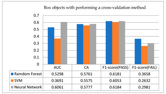 Figure 8. Cross-validation results for box objects.
 - (2)
- Results for cylinder objects: Figure 9 shows the results for the cross-validation index score of three algorithms used on the cylindrical objects. From Figure 9, we observe that in this cylindrical object, the three algorithms have achieved a CA rate higher than 0.65, the RF is as high as 0.712, and the performance of RF and SVM is better than random guessing (i.e., 0.5). However, the AUC part of the ANN is lower than random guessing for this cylindrical object. This situation is worthy of further research by subsequent scholars. Moreover, what is more serious when compared with box objects in Figure 8 is that the F1-score results of a sintering failure obtained by these three algorithms are all lower than those obtained by boxes, and the possible reason is also worthy of further investigation in the future.
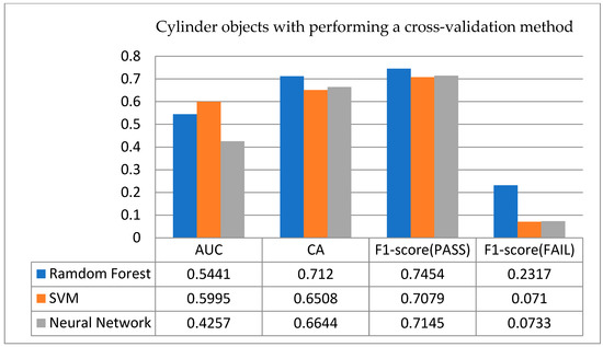 Figure 9. Cross-validation results for cylinder objects.
 - (3)
- Results for flat objects: The cross-validation results with score indicators for three algorithms used in the flat objects, are shown in Figure 10. In terms of AUC, the three algorithms are similar to random guessing, and in terms of CA rate, the ANN has the highest accuracy rate of 0.6712; but in terms of F1-score, it is found that the F1-score of a sintering failure for these three algorithms is close to 0, and even the ANN is 0, which means that in this confusion matrix, the number of samples successfully predicted as a sintering failure is 0.
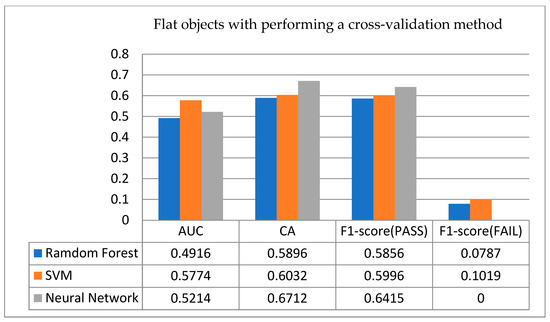 Figure 10. Cross-validation results for flat objects.
 - (4)
- Results for total-result objects: As for the results of the total-result objects, Figure 11 shows their cross-validation results. In the AUC part, the ANN shows better performance than random guessing; as for the CA rate, the ANN has the highest accuracy rate, reaching nearly 0.6, which is higher than the classification performance of the other two classifiers. After observing the F1-score, it is found that the results obtained for this object are different from those obtained for the other three objects. In the other three objects, the probability of sintering success is much higher than that of sintering failure. However, it has the opposite case in this total-result object. That is, a sintering failure is higher than a sintering success, but the gap in rate between a sintering failure and a sintering success is not large.
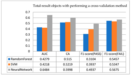 Figure 11. Cross-validation results for total-result of all objects.
Summarizing the above four results, we get the important results of implementing the cross-validation method, and there are fewer objects on the sintering failure of cylinders (17) and flats (18), so that the cross-validation results may directly be classified as successful sintering. Although such results can get a relatively high accuracy rate, they cannot faithfully present the real situation; thus, we need to perform an oversampling operation for the given data on each sintered object to solve the imbalance problem for two classes (fail and pass), and then compare the difference between each verification index with/without an oversampling method. The comparison results are shown in the next section.
4.3. Oversampling Results for Sintering Objects
For the empirical results of testing sintering objects, we still differentiate four different object purposes by identifying and illustrating their performance with/without an oversampling technique for the given data, respectively.
- (1)
- Box objects: Provide the testing data to the established model and experiment operations, and observe the experimental results. Figure 12 shows a comparison of testing results with/without using an oversampling technique for box objects. Figure 12 (above) is the result obtained by verifying the no-oversampling data of samples for the box objects. In particular, from Figure 12 (above), there are three key points identified. (a) The accuracy rates of the three classification algorithms used are all above 0.6, and the highest are the SVM (0.6334) and the ANN (0.6333); (b) Moreover, the scores of the F1-score are all around 0.6. (c) In terms of AUC, the ANN is the highest, followed by the RF, and finally the SVM, and the SVM is even worse when compared to random guessing. To identify the difference between with/without using an oversampling method, this experiment adds the oversampling technique. Figure 12 (below) presents the empirical results with a data oversampling method; as a result, there are some key points identified from it. (a) The accuracy of the SVM and the ANN is improved to 0.6501 and 0.6668, respectively; from the CA results, it is found that the data processed by the oversampling technique is more helpful to the ANN in this box object. On the contrary, it is the least effective for RFs, and the accuracy rate does not increase but decreases. With this interesting result, it is a valuable issue to further explore in the future. (b) As an AUC indicator, the ranking is SVM ➔ ANN ➔ RF, just conversely without using an oversampling technique, and the three algorithms are better than random guessing. (c) On the F1-score, the ANN and SVM have improved, from 0.598 to 0.6644 and from 0.6085 to 0.6482, respectively. Finally, summarizing the empirical results on this box object from Figure 12, there are better testing results using an oversampling technique to conclude that the classification performance has been significantly improved.
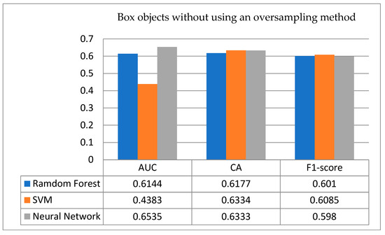
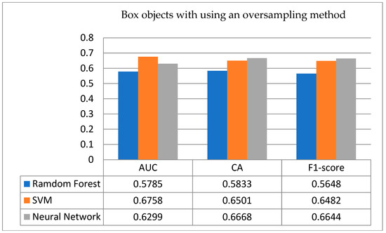 Figure 12. Testing results with/without using an oversampling technique for box objects.
Furthermore, Table 2 shows the classification results of box objects with/without an oversampling technique for the sample sets that are successfully sintered. From the comparison of statistical quantities, it is known that both the ANN and the SVM have one case of data that directly predicts the result of the sample set as sintering success when the 10 sample sets are not oversampled, while the RF has two cases of data. However, in the prediction after the oversampling technique, none of the sample sets are predicted as successful sintering, and the accuracy of the ANN is improved, which means that the accuracy of the prediction of a sintering failure is improved.
Table 2.
The information whose classification results are all successfully entered in the box sample set.
- (2)
- Cylindrical objects: Figure 13 shows the comparison with/without using an oversampling technique for testing the results of cylindrical objects. As shown in Figure 13 (above), the accuracy rates of these three classification algorithms are all higher than 0.7, among which the highest CA rate is 0.7499 for RF, 0.7167 for ANN, and 0.70 for SVM. In terms of the AUC evaluator, it is found that only the SVM is better than random guessing; however, in the F1-score indicator, the ranking of the three classification algorithms is the same as that of the CA rate. That is RF ➔ ANN ➔ SVM, and all the scores are above 0.63. From Figure 13 (below), there are two key directions identified. (a) After implementing the oversampling technique, it is found that only the performance of the RF is improved, while both the performances of the SVM and the ANN are reduced; this special case represents that when the model is changed, there may be an overfitting problem with the prediction data. (b) Among them, there exists one special thing: the accuracy of the RF remains unchanged, but the F1-score and AUC show a decline in terms of most performances. This interesting point is also worth further exploring the possible reasons in the future.
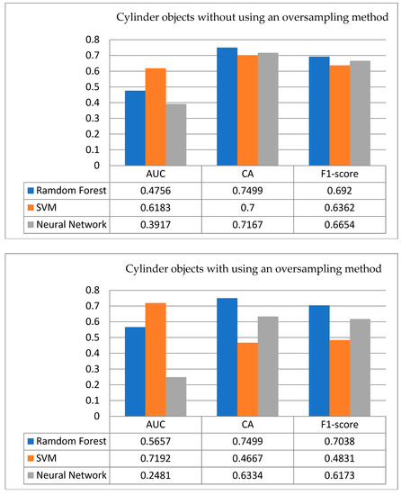 Figure 13. Testing results for cylindrical objects with/without an oversampling method.
Furthermore, Table 3 shows the classification results with/without an oversampling technique of successful sintering for cylindrical objects in the sample set. From its statistical outcome, in the 10 sample sets that have not been oversampled, both the ANN and the RF have six cases that directly predict a successful sintering case of the sample set, while there are five cases in the RF. However, in the prediction work after the oversampling technique, the number of sample data points that were originally classified as successful sintering has decreased significantly. In particular, the CA rate in the RF remains unchanged; this interesting phenomenon represents that this classification model is good, and the empirical result is more in line with the real situation and closer to the status quo.
Table 3.
The information whose classification results are all successful sintering in the cylindrical sample set.
- (3)
- Flat objects: Figure 14 shows the comparison of testing results for the flat objects with/without treatment using an oversampling technique. From Figure 14 (above), the accuracy rate and F1-score in the ANN without using an oversampling technique are higher than those of the other two classification models; however, only in the AUC indicator is it lower than the SVM, and it is inferior to random guessing. In exploring the possible reasons, it is possible that due to the unbalanced categories of the original training data, all classifiers predict the sintering result as successful, resulting in higher accuracy. However, in practice, the expected results cannot be achieved, which is compared and seen from the cross-validation method of flat objects. In Figure 14 (below), after using the oversampling technique, it is strange that the accuracy rates of the ANN and the SVM are greatly reduced to 0.4499 and 0.4334, respectively; however, the RF is just the opposite, and its accuracy rate has slightly improved from 0.6333 to 0.6499. Both the F1-score and AUC have also increased slightly to 0.6262 and 0.5163, respectively. Moreover, from the above empirical results, we discover a very interesting fact: on flat objects, when the data classes are more unbalanced and after implementing the oversampling technique of data, the RF gets a relatively good classification performance.
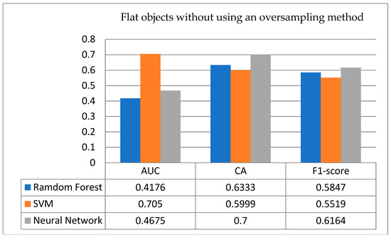
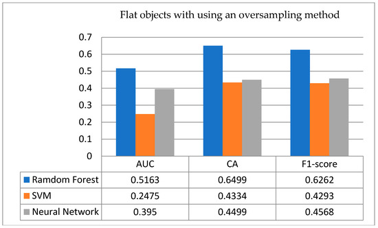 Figure 14. Testing results for flat objects with/without using an oversampling technique.
Accordingly, Table 4 shows the classification results of sample sets for flat objects with/without using an oversampling method with successful sintering. From Table 4, we count that among the 10 un-oversampled sample sets, the results of eight, four, and six sample sets of the ANN, RF, and SVM are directly predicted as successful sintering, respectively. However, in the prediction, after implementing the oversampling technique, the number of sample data points that are all classified as successful sintering is reduced. In this flat object, the accuracy rate of the RF has increased, and this special case means that the accuracy rate of predicting a sintering failure has increased, which implies that the classification model is more in line with the reality of 3D-SLS for the case company.
Table 4.
The information whose classification results are all successfully sintered in the flat sample set.
- (4)
- Total result of summarized objects: In yield prediction for SLS on the total result of sintered objects, Figure 15 shows the comparison of testing results for summarized objects with/without sample augmentation. Through Figure 15 (above), it is observed that when there is no processing sample augmentation, the ANN performance is higher than the other two listed models regardless of indicators of AUC, CA rate, and F1-score; therefore, the prediction ability of the ANN model is the best performer. However, in Figure 15 (below), the CA rate of the ANN after implementing the sample data augmentation method has dropped to 0.5668, the F1-score has dropped to 0.525, and the AUC has dropped to 0.5556. On the contrary, the indicators of AUC, CA rate, and F1-score for the RF are increased to 0.5777, 0.5834, and 0.5468, respectively; similarly, all the performances of the SVM are also improved. However, since there is no serious class unbalance problem in the total result of summarizing objects, the function of an oversampling technique is not performed; the data is directly expanded to more than 200 items. Unfortunately, such an approach may lead to overfitting problems in these models; in this total result of the cross-validation method, the ANN has also achieved the best result in this research. Thus, we can clearly express that in this model, the ANN can still be used as a predictive model, and in the overall result, the best performance result is the ANN model.
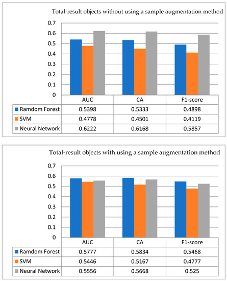 Figure 15. Test results for objects summary processed with/without sample data augmentation.
Subsequently, Table 5 shows the classification results of the total-result object sample sets with/without sample data expansion for a successful sintering. From Table 5, no matter whether sample data has been expanded or not, there is no sample of the sintering results, which is classified into the sample set of a successful sintering. After data expansion, the CA rate of the ANN has decreased significantly, while the accuracy of the RF and SVM has increased, however, they are not higher than the un-augmented ANN.
Table 5.
The information in which the classification results are all successfully sintered in the total-result sample set.
More importantly, this research thus concludes with two core directions for the overall results. (1) It is unnecessary for the total-result objects to perform data expansion processing. (2) However, in the prediction results for box, cylinder, and flat objects, it is absolutely necessary to perform data processing using an oversampling technique because it can reduce the case that the sintering results are all predicted as successful sintering, and it can make the predicted results closer to the actual situation of SLS and increase the plasticity and credibility of these classification models.
4.4. Comparison Results for Sintering Times and Adjustment Times before and after the Modification of Verification Process
Consequently, this research first calculates the comparison of sintering times for the proposed model. To facilitate the follow-up comparison operation, we assume that the sintering will be successful in the second sintering, then count the number of sintering times based on the predicted results, and further compare the number of sintering times obtained before and after the modification of the verification process. By the previous testing sample data in Table 1, we know that there are six testing samples each time; in the data set of the total-result objects, there are three samples of failed sintering and three samples of successfully sintered. Looking at this combination again, the verification process before modification needs to be sintered nine times (3 + 3 × 2) before the six samples are successfully verified. As a result, Figure 16 shows the statistical results of sintering times for each data set after the modification.
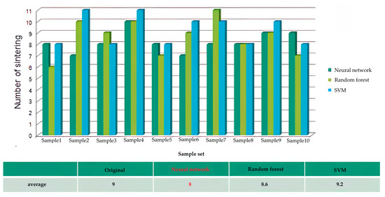
Figure 16.
Statistical results of sintering times for the modified verification process for each sample data set.
From Figure 16, we get the number of sintering times for each classification model. Interestingly, the number of sintering times for the ANN is reduced by one time (i.e., eight times) on average in each sample set; especially in the first and second sample sets, the sintering times of the verification process before and after the modification are the same, except the seventh sample set is sintered once more after the modification than the verification process before the modification, and the sintering times of other sample sets are the same. Thus, it is less than nine times, so the average number of sintering times is calculated as eight times for the ANN model. The average sintering times for the modified verification process of the ANN outperform the verification process before the modification and that of other classification models: RF and SVM. Especially, SVM (9.2 times) is even worse than the original verification process (9.0 times) before the modification, and the potential reason is also worthy of further exploration in the future.
Subsequently, in the comparison of the number of adjustment times after quantifying the oversampled data results, Figure 17 shows the number of prediction adjustment times for the three classifiers on each testing data set. By observing Figure 17, we know that among the 10 sample sets, the average number of adjustments for the RF is the least, and each test sample set has an average adjustment of 10.7 times, while the average adjustment times of the ANN and SVM are 11.7 times and 13.5 times, respectively. In terms of the number of adjustment times, it is found that the RF model yields fewer adjustments than the other two models; thus, RFs perform the best in terms of the number of adjustment times for this research case.
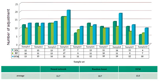
Figure 17.
Information on adjustment times for the three classifiers in each testing data set.
More importantly, through the above empirical results, the following key points are sorted out: (1) It is found that the best verification process is to use the ANN that has not been processed by the oversampling technique to forecast the total-result objects. (2) Use the RF model obtained after an oversampling method to predict the sintering results for each sintered object and to train out the parameters of the best model. (3) After doing the above operations, the study models proposed are used to effectively carry out the best verification process with the least number of sintering times and the least number of adjustment times, which is one of the major contributions of this research for experiencing industrial data analysis and application.
4.5. Empirical Summary of All Results for the Experiments with Discussions
Totally, we use five directions to uniformly illustrate the primary outcome of the empirical summary with some meaningful discussions and values after executing all the experiments in this research, as follows:
- (1)
- Key experimental results of objects: in the mathematical experiment operations based on the cross-validation method, we have identified and summarized the following four main points: (a) On the box objects: the evaluation indicators of the ANN are the best, and the results of three indicators are AUC 0.50, CA rate 0.57, and F1-scores of a sintering success of 0.61 and a sintering failure of 0.30. (b) On the cylindrical objects: the evaluation indicators of RF are the best, and the three indicators are described as AUC 0.54, CA rate 0.71, and F1-score of a sintering success of 0.74 and a sintering failure of 0.23. (c) On the flat objects: ANNs have the best performance results, and the evaluation indicators are AUC 0.52, CA rate 0.67, and F1-score of a sintering success of 0.64 and a sintering failure of 0. (d) On the total-result objects: the performance results are the same as those of flat objects, and the experimental results of the ANNs model are also the best. The evaluation indicators are identified as AUC 0.65, CA rate 0.60, and F1-scores of a sintering success of 0.50 and a sintering failure of 0.56.
- (2)
- Gaps of the cross-validation method: regarding the cross-validation method, the result for the gap of the F1-score between the sintering success and the sintering failure for the three objects is too large, which means that most mathematical binary classification models are still more inclined to classify the data as sintering success.
- (3)
- Differences with/without using an oversampling technique: we obtain the following four core values for the gaps with/without the oversampling technique: (a) In the case of box objects: the best CA is to use the ANN model; after using the oversampling technique, its CA is increased from 0.6333 to 0.6668, and the F1-score is increased from the original 0.587 to 0.6644. (b) In the case of cylindrical objects: the highest CA is 0.7499 in the RF, its AUC is increased from 0.4756 to 0.5657, and its F1-score is increased from 0.6920 to 0.7038. (c) In the case of flat objects: the best CA is the ANN when the samples have un-oversampled data. However, after implementing the oversampling technique, the CA of ANN is not rising but falling, and even lower than 0.5; interestingly, the RF has achieved the highest CA from 0.6333 to 0.6499, the highest F1-score from 0.5847 to 0.6262, and the lowest AUC from less than 0.5 to 0.5163. (e) In the case of total-result objects: the ANN model without sample data expansion has the highest CA of 0.6168, AUC of 0.6222, and F1-score of 0.5857. However, after expanding the sample data, the highest CA for the total-result objects is the RF model, which has increased from 0.5333 to 0.5834; the F1-score has increased from 0.4898 to 0.5468; and the AUC indicator has also increased from 0.5389 to 0.5777.
- (4)
- Reduction of time and times: After integrating the experiment results and comparing them with the original manufacturing process time, it is found that each machine reduces the sintering time by an average of four hours. Moreover, if the sampling of the data used is expanded, it is more suitable to use the RF algorithm when predicting the sintering failure of the objects, and its average number of sintering times per machine is 1.70 times, which is better than 1.95 times for the ANN and 2.25 times for the SVM.
- (5)
- Results of sample data expansion: the result of the cross-validation method for the total-result objects does not have the serious problem of class imbalance; thus, using the sample data expansion method instead of the oversampling method is suitable. Especially in this case, there are two core concerns identified. (a) This research confirms that in each given data set, the ANN without sample expansion can reduce the sintering verification by one time. (b) After processing the sample expansion method, the RF for the failure prediction of objects gets a minimum of 10.7 times of adjustments, which is lower than the 11.7 and 13.5 of the ANN and SVM, respectively.
5. Research Findings and Research Limitations
It is necessary to identify two types of research concerns for further aggregating the study results mentioned above, including research findings and research limitations, in order to benefit from and highlight the study issue of the SLS manufacturing process, as follows.
5.1. Important Research Findings
In summarizing the empirical study results of this research in the field of industrial data analysis, the following key research findings have been defined, and these findings can provide a useful reference for relevant industry applications and academic circles.
- (1)
- As a total result of object prediction, this research finds that it is not absolutely necessary to carry out data expansion processing on samples. However, in the mathematical prediction of experiment results for box, cylinder, and flat objects, it is necessary to perform an oversampling technique because this technique can solve the problem that the sintering results are all predicted to be sintering successes, making the prediction results more accurate and real. The closeness to the factual situation can increase the plasticity and credibility of the mathematical classification model.
- (2)
- In terms of the number of adjustment times in this research case, it is found that the performance of the RF model is the best. Thus, it is recommended that follow-up operators simulate and use the constructed RF model if they are more focused on reducing the number of adjustment times for identifying the SLS yield.
- (3)
- In the empirical results, it is found that the best verification process is to use the ANN model that has not been processed by the oversampling technique as the prediction of the total result for the objects sintered.
- (4)
- In the CA for the modified verification process, it is found that the average performance of the ANN is better than that before the modification, and its verification process of the binary classification model is better than the other listed models, followed by the RF, and finally the SVM; that is, in the ranking of ANN ➔ RF ➔ SVM.
- (5)
- If the sample data is processed by an oversampling technique, it is found that the RF model in this research is the best to optimize the parameters used to predict the sintering failure of each sintered object. After performing the above operations, the proposed mathematical binary classification model effectively carries out and appropriately obtains the best verification process with the least number of sintering times and the least number of machine parameter adjustments for interested parties.
5.2. Research Limitations
The focus of this research is the SLS manufacturing process, and there are three potential research limitations identified.
- (1)
- Due to many shortcomings in sintering the SLS products, such as the high unit price of machine equipment, the high construction cost of the sintering environment, and the high sintering cost, these major defects result in a limited application value: the sales volume of the machine (already a niche market) has shrunk even more, and even this makes companies daunting. Due to the high costs of purchasing this equipment, general business is discouraged. This special situation causes the sample data to be relatively scarce; thus, the small amount of raw sample data has also become the first main research limitation for this research.
- (2)
- For manufacturers of SLS machines, the verification results of machine output are a huge expense; thus, the data of each verification record is an expensive and valuable experience. Given this reason, general SLS manufacturers mainly hope to reduce the number of sintering times in order to lower the high verification cost of the machine output. Thus, enhancing the one-time sintering greatly lowers the operating burden on the manufacturer. The high verification cost creates a bottleneck problem in data collection, and this problem is serious and is the second research limitation.
- (3)
- The third research limitation is that the example of the research objects is only from a certain SLS company, which may result in a lack of diversity of sample data and an inference limitation of research results.
6. Conclusions and Future Research
To overcome the serious problems when forming the sintering of a standard SLS object, this research has constructed a mathematical prediction system to reduce the time and cost of sintering verification. The following two sections give the core highlights of empirical conclusions with contributions and future prospects, respectively.
6.1. Empirical Conclusions with Industrial Contribution
After all the experiments, we have concluded that the following two key contributions were integrated into the study conclusions:
- (1)
- Industrial contribution: this research is mainly aimed at realizing an effective prediction framework for identifying SLS yield, which is mainly used to reduce the sintering time cost and direct material cost of the verification process. The ability of proposed mathematical binary classification models for each object is evaluated through the cross-validation method, and their accuracy is verified by actual data collected from a case study for industrial applications. Thus, through the above empirical results, the number of sintering times is reduced. Importantly, although this research has not provided an innovative technique, such a binary model constructed is rarely seen in the SLS industry for 3D-AM issues, and it has made a great industrial contribution by effectively reducing the verification cost of the SLS manufacturing process in practice.
- (2)
- Applicable values: the proposed mathematical binary models in this research make the prediction of the SLS yield more accurate to reduce the situation that the prediction results are all predicted to be sintering success, and to be closed to the real case of industries, it is proved that the mathematical binary model has the superiority of its application performance in industrial manufacturing processes. Thus, it also has significant applicable values based on the empirical results of industrial data analysis.
6.2. Future Research
Although the experimental performance of this research has research advantages and benefits and the empirical results are remarkable, there are still some rooms for improvement in the future, and these improvements can provide references for subsequent directions to interested researchers or industry requirements, as follows:
- (1)
- The first improvement is about the diversity of molding materials; these materials have different material properties, molding parameters, and shrinkage rates. Since the main material of this research is PA12 (Polyamide 12 powder for SLS printing material) [10,30], subsequent researchers can use materials different from PA12, and the new material may not be able to adapt to the optimized parameters of the proposed binary classification model. Therefore, we suggest that new types of materials are added into the proposed models as new features (factors), and after collecting sample data, data retraining and data retesting are conducted to further measure the classification performance and efficiency of the binary classification model.
- (2)
- In the practical sintering application, since the sintering result is not only determined by the dimensional size accuracy but also requires other measurements of unique characteristics of different materials, such as the range of strength and toughness or the density detection of the objects, these results directly or indirectly lead to molding whether the object is successful. Thus, it is suggested that subsequent researchers can collect the above different data, add it to the proposed models, and then re-predict the forming results of the SLS manufacturing process.
- (3)
- The biggest problem in this research is that the amount of SLS practical sample data is insufficient, causing insufficient training data, which directly affects the prediction results. Thus, it is recommended to collect more raw samples of data to retrain the mathematical binary classification model and address future directions.
- (4)
- In some large machine tools, it is a common problem that obtaining the sample data is difficult; thus, it is suggested that the models of how to predict with a small amount of data should be further focused in the future. It is a feasible alternative to use the GAN method to create more fake sample data of a sintering failure to increase the sample number for sufficiently training the binary model and improving its performance.
- (5)
- For the RF algorithm, it also has a feature importance score, which can help gain insight into which features are important. Thus, the RF can be used for the technique of FS to reduce the dimensionality of data to select the best features [57]. For this reason, the RF can be added to the proposed model to further remove irrelative features, facilitate experiment operations, and measure its model performance in the future.
- (6)
- Finally, this research is still committed to constructing a set of classification frameworks to judge sintering result strategies in a process-based structure of automatic and intelligent methods. The purpose is that researchers can regard the proposed models as a basis to develop their future models for comprehensive comparison with more techniques of the state of the art, such as Xgboost or K shot. Moreover, the establishment of the maintenance strategy for sintering enables the adjustment of machine parameters to be more automatic and intelligent, with effective and efficient effects.
Author Contributions
Conceptualization, J.-R.C. and Y.-S.C.; Methodology, J.-R.C. and Y.-S.C.; Software, J.-H.L. and Y.-H.H.; Visualization, J.-R.C., Y.-S.C. and Y.-H.H.; Writing—original draft, J.-H.L., J.-R.C. and Y.-S.C.; Writing—review and editing, Y.-S.C. and Y.-H.H. All authors have read and agreed to the published version of the manuscript.
Funding
This research was partially supported by the National Science and Technology Council of Taiwan for grant number NSTC 111-2221-E-167-036-MY2.
Data Availability Statement
Not applicable.
Conflicts of Interest
The authors declare no conflict of interest.
Appendix A
Table A1.
Information of 65 records of raw data.
Table A1.
Information of 65 records of raw data.
| Serial No. | Z at 239.9 mm Accuracy | Spot Size (um) | The Max. Error of the X-Axis Galvanometer | The Max. Error of the Y-Axis Galvanometer | Laser Energy 50% | Box | Cylinder | Flat | Total-Result |
|---|---|---|---|---|---|---|---|---|---|
| 1 | 0.09 | 525 | 0.22 | 0.31 | 23.35 | fail | pass | fail | fail |
| 2 | 0.09 | 515 | 0.33 | 0.27 | 22.26 | fail | fail | fail | fail |
| 3 | 0.11 | 555 | 0.28 | 0.28 | 20.72 | pass | pass | fail | fail |
| 4 | 0.12 | 545 | 0.18 | 0.22 | 21.38 | pass | pass | fail | fail |
| 5 | 0.10 | 545 | 0.27 | 0.31 | 22.79 | pass | pass | fail | fail |
| 6 | 0.10 | 575 | 0.30 | 0.35 | 20.79 | fail | pass | fail | fail |
| 7 | 0.10 | 555 | 0.23 | 0.24 | 18.02 | pass | fail | fail | fail |
| 8 | 0.11 | 565 | 0.31 | 0.23 | 20.93 | fail | pass | pass | fail |
| 9 | 0.10 | 545 | 0.24 | 0.31 | 21.46 | fail | fail | pass | fail |
| 10 | 0.10 | 575 | 0.31 | 0.22 | 18.29 | fail | pass | pass | fail |
| 11 | 0.10 | 565 | 0.19 | 0.26 | 21.62 | fail | pass | pass | fail |
| 12 | 0.11 | 545 | 0.33 | 0.20 | 20.74 | fail | pass | fail | fail |
| 13 | 0.09 | 535 | 0.25 | 0.31 | 20.47 | fail | pass | fail | fail |
| 14 | 0.11 | 525 | 0.33 | 0.28 | 22.99 | fail | pass | pass | fail |
| 15 | 0.11 | 505 | 0.25 | 0.26 | 22.20 | pass | pass | fail | fail |
| 16 | 0.11 | 515 | 0.26 | 0.22 | 23.67 | fail | pass | pass | fail |
| 17 | 0.12 | 535 | 0.34 | 0.33 | 22.23 | fail | fail | fail | fail |
| 18 | 0.09 | 555 | 0.21 | 0.26 | 18.66 | fail | fail | fail | fail |
| 19 | 0.11 | 555 | 0.23 | 0.20 | 22.09 | fail | pass | pass | fail |
| 20 | 0.12 | 515 | 0.21 | 0.18 | 21.75 | fail | pass | fail | fail |
| 21 | 0.11 | 535 | 0.27 | 0.29 | 21.88 | fail | fail | pass | fail |
| 22 | 0.10 | 545 | 0.32 | 0.21 | 22.52 | fail | pass | pass | fail |
| 23 | 0.08 | 555 | 0.24 | 0.32 | 20.25 | fail | pass | pass | fail |
| 24 | 0.11 | 555 | 0.33 | 0.33 | 24.33 | fail | fail | pass | fail |
| 25 | 0.10 | 525 | 0.27 | 0.24 | 22.18 | fail | pass | pass | fail |
| 26 | 0.10 | 515 | 0.22 | 0.26 | 23.49 | pass | fail | fail | fail |
| 27 | 0.10 | 545 | 0.33 | 0.28 | 23.18 | pass | fail | fail | fail |
| 28 | 0.12 | 535 | 0.25 | 0.31 | 19.58 | fail | pass | pass | fail |
| 29 | 0.10 | 535 | 0.28 | 0.27 | 21.52 | fail | pass | pass | fail |
| 30 | 0.12 | 515 | 0.21 | 0.25 | 23.36 | pass | fail | pass | fail |
| 31 | 0.11 | 545 | 0.18 | 0.14 | 22.23 | pass | fail | pass | fail |
| 32 | 0.11 | 525 | 0.26 | 0.22 | 20.89 | pass | fail | pass | fail |
| 33 | 0.09 | 535 | 0.26 | 0.20 | 22.45 | fail | fail | fail | fail |
| 34 | 0.10 | 565 | 0.23 | 0.30 | 23.32 | pass | fail | fail | fail |
| 35 | 0.10 | 545 | 0.18 | 0.15 | 22.41 | pass | fail | fail | fail |
| 36 | 0.09 | 515 | 0.21 | 0.33 | 23.75 | fail | fail | pass | fail |
| 37 | 0.10 | 545 | 0.20 | 0.18 | 25.86 | fail | fail | pass | fail |
| 38 | 0.10 | 535 | 0.32 | 0.26 | 20.52 | pass | pass | pass | pass |
| 39 | 0.10 | 525 | 0.32 | 0.21 | 21.03 | pass | pass | pass | pass |
| 40 | 0.10 | 555 | 0.27 | 0.26 | 19.90 | pass | pass | pass | pass |
| 41 | 0.10 | 525 | 0.28 | 0.32 | 21.56 | pass | pass | pass | pass |
| 42 | 0.11 | 525 | 0.18 | 0.27 | 22.19 | pass | pass | pass | pass |
| 43 | 0.09 | 545 | 0.30 | 0.31 | 21.13 | pass | pass | pass | pass |
| 44 | 0.10 | 535 | 0.26 | 0.23 | 22.50 | pass | pass | pass | pass |
| 45 | 0.10 | 545 | 0.21 | 0.23 | 22.30 | pass | pass | pass | pass |
| 46 | 0.12 | 555 | 0.27 | 0.255 | 21.13 | pass | pass | pass | pass |
| 47 | 0.11 | 525 | 0.24 | 0.24 | 22.08 | pass | pass | pass | pass |
| 48 | 0.10 | 555 | 0.18 | 0.24 | 25.09 | pass | pass | pass | pass |
| 49 | 0.11 | 575 | 0.28 | 0.20 | 22.80 | pass | pass | pass | pass |
| 50 | 0.11 | 615 | 0.25 | 0.28 | 24.72 | pass | pass | pass | pass |
| 51 | 0.11 | 535 | 0.26 | 0.26 | 22.97 | pass | pass | pass | pass |
| 52 | 0.10 | 525 | 0.24 | 0.28 | 26.70 | pass | pass | pass | pass |
| 53 | 0.12 | 515 | 0.30 | 0.26 | 24.54 | pass | pass | pass | pass |
| 54 | 0.11 | 545 | 0.26 | 0.21 | 22.87 | pass | pass | pass | pass |
| 55 | 0.10 | 545 | 0.17 | 0.24 | 23.65 | pass | pass | pass | pass |
| 56 | 0.11 | 515 | 0.22 | 0.23 | 22.34 | pass | pass | pass | pass |
| 57 | 0.10 | 575 | 0.24 | 0.26 | 23.81 | pass | pass | pass | pass |
| 58 | 0.11 | 555 | 0.26 | 0.32 | 22.07 | pass | pass | pass | pass |
| 59 | 0.11 | 515 | 0.30 | 0.30 | 21.83 | pass | pass | pass | pass |
| 60 | 0.10 | 565 | 0.27 | 0.25 | 21.88 | pass | pass | pass | pass |
| 61 | 0.11 | 545 | 0.18 | 0.26 | 21.60 | pass | pass | pass | pass |
| 62 | 0.09 | 525 | 0.15 | 0.26 | 21.27 | pass | pass | pass | pass |
| 63 | 0.11 | 595 | 0.23 | 0.26 | 21.68 | pass | pass | pass | pass |
| 64 | 0.10 | 595 | 0.27 | 0.32 | 22.61 | pass | pass | pass | pass |
| 65 | 0.10 | 535 | 0.20 | 0.20 | 23.67 | pass | pass | pass | pass |
References
- Fina, F.; Goyanes, A.; Gaisford, S.; Basit, A.W. Selective laser sintering (SLS) 3D printing of medicines. Int. J. Pharm. 2017, 529, 285–293. [Google Scholar] [CrossRef] [PubMed]
- Schmid, M.; Amado, A.; Wegener, K. Polymer Powders for Selective Laser Sintering (SLS). In AIP Conference Proceedings, Cleveland, OH, USA, 6–12 June 2014; AIP Publishing LLC: New York, NY, USA, 2015; Volume 1664, p. 160009. [Google Scholar] [CrossRef]
- Wai Ming, L.; Gibson, I. Possibility of colouring SLS prototypes using the ink-jet method. Rapid Prototyp. J. 1999, 5, 152–154. [Google Scholar] [CrossRef]
- Kruth, J.P.; Wang, X.; Laoui, T.; Froyen, L. Lasers and materials in selective laser sintering. Assem. Autom. 2003, 23, 357–371. [Google Scholar] [CrossRef]
- Kumar, S. Selective laser sintering: A qualitative and objective approach. JOM 2003, 55, 43–47. [Google Scholar] [CrossRef]
- Gibson, I.; Shi, D. Material properties and fabrication parameters in selective laser sintering process. Rapid Prototyp. J. 1997, 3, 129–136. [Google Scholar] [CrossRef]
- Wang, X. Calibration of shrinkage and beam offset in SLS process. Rapid Prototyp. J. 1999, 5, 129–133. [Google Scholar] [CrossRef]
- Reddy, T.J.; Kumar, Y.R.; Rao, C.S.P. Determination of Optimum Process Parameters Using Taguchi’s Approach to Improve the Quality of SLS Parts. In Proceedings of the 17th IASTED International Conference on Modelling and Simulation (MS’06), Montreal, QC, Canada, 24–26 May 2006; pp. 228–233. [Google Scholar]
- Shi, Y.; Li, Z.; Sun, H.; Huang, S.; Zeng, F. Effect of the properties of the polymer materials on the quality of selective laser sintering parts. Proc. Inst. Mech. Eng. L J. Mater. Des. Appl. 2004, 218, 247–252. [Google Scholar] [CrossRef]
- Muhamad Damanhuri, A.A.; Md Fauadi, M.H.F.; Hariri, A.; Alkahari, M.R.; Omar, M.R. Emission of selected Environmental Exposure from Selective Laser Sintering (SLS) Polyamide Nylon (PA12) 3D printing Process. J. Saf. Health Ergon. 2019, 1, 1–6. Available online: http://fazpublishing.com/jshe/index.php/jshe/article/view/1/5 (accessed on 11 October 2022).
- Lopes, A.C.; Sampaio, Á.M.; Silva, C.S.; Pontes, A.J. Prediction of SLS parts properties using reprocessing powder. Rapid Prototyp. J. 2021, 27, 496–506. [Google Scholar] [CrossRef]
- Atluri, G.; Karpatne, A.; Kumar, V. Spatio-temporal data mining: A survey of problems and methods. ACM Comput. Surv. 2018, 51, 1–41. [Google Scholar] [CrossRef]
- Wang, S.; Cao, J.; Philip, S.Y. Deep learning for spatio-temporal data mining: A survey. IEEE Trans. Knowl. Data Eng. 2020, 34, 3681–3700. [Google Scholar] [CrossRef]
- Xiao, L.; Lu, M.; Huang, H. Detection of powder bed defects in selective laser sintering using convolutional neural network. Int. J. Adv. Manuf. Technol. 2020, 107, 2485–2496. [Google Scholar] [CrossRef]
- Guo, Y.; Lu, W.F.; Fuh, J.Y.H. Semi-supervised deep learning based framework for assessing manufacturability of cellular structures in direct metal laser sintering process. J. Intell. Manuf. 2021, 32, 347–359. [Google Scholar] [CrossRef]
- Stathatos, E.; Vosniakos, G.C. Real-time simulation for long paths in laser-based additive manufacturing: A machine learning approach. Int. J. Adv. Manuf. Technol. 2019, 104, 1967–1984. [Google Scholar] [CrossRef]
- Shen, X.; Yao, J.; Wang, Y.; Yang, J. Density Prediction of Selective Laser Sintering Parts Based on Artificial Neural Network. In Proceedings of the ISNN 2004: International Symposium on Neural Networks Part II 1, Dalian, China, 19–21 August 2004; Yin, F.L., Wang, J., Guo, C., Eds.; Advances in Neural Networks. Springer: Berlin/Heidelberg, Germany; Volume 3174, pp. 832–840. [Google Scholar] [CrossRef]
- La Fé-Perdomo, I.; Ramos-Grez, J.A.; Jeria, I.; Guerra, C.; Barrionuevo, G.O. Comparative analysis and experimental validation of statistical and machine learning-based regressors for modeling the surface roughness and mechanical properties of 316L stainless steel specimens produced by selective laser melting. J. Manuf. Process. 2022, 80, 666–682. [Google Scholar] [CrossRef]
- Sharifani, K.; Amini, M. Machine learning and deep learning: A review of methods and applications. World Inf. Technol. Eng. J. 2023, 10, 3897–3904. [Google Scholar]
- Zhu, M.; Yang, Y.; Feng, X.; Du, Z.; Yang, J. Robust modeling method for thermal error of CNC machine tools based on random forest algorithm. J. Intell. Manuf. 2023, 34, 2013–2026. [Google Scholar] [CrossRef]
- Kurani, A.; Doshi, P.; Vakharia, A.; Shah, M. A comprehensive comparative study of artificial neural network (ANN) and support vector machines (SVM) on stock forecasting. Ann. Data Sci. 2023, 10, 183–208. [Google Scholar] [CrossRef]
- Yan, C.; Shi, Y.; Hao, L. Investigation into the differences in the selective laser sintering between amorphous and semi-crystalline polymers. Int. Polym. Process. 2011, 26, 416–423. [Google Scholar] [CrossRef]
- Chen, P.; Cai, H.; Li, Z.; Li, M.; Wu, H.; Su, J.; Wen, S.; Zhou, Y.; Liu, J.; Wang, C.; et al. Crystallization kinetics of polyetheretherketone during high temperature-selective laser sintering. Addit. Manuf. 2020, 36, 101615. [Google Scholar] [CrossRef]
- Hassan, M.S.; Billah, K.M.M.; Hall, S.E.; Sepulveda, S.; Regis, J.E.; Marquez, C.; Cordova, S.; Whitaker, J.; Robison, T.; Keating, J.; et al. Selective laser sintering of high-temperature thermoset polymer. J. Compos. Sci. 2022, 6, 41. [Google Scholar] [CrossRef]
- Mojaddarasil, M.; Kiani, A.; Tavakoli, M.R.; Badrossamay, M. A parametric study of powder bed temperature distribution in selective laser sintering process. J. Mater. Eng. Perform. 2023, 32, 3348–3367. [Google Scholar] [CrossRef]
- Sharma, V.; Singh, J.; Sharma, V.S.; Sachdeva, A.; Gupta, M.K.; Singh, S. Investigations on mechanical properties of polyamide parts fabricated by selective laser sintering process. J. Mater. Eng. Perform. 2022, 31, 5767–5781. [Google Scholar] [CrossRef]
- Chavez, L.A.; Ibave, P.; Hassan, M.S.; Hall-Sanchez, S.E.; Billah, K.M.M.; Leyva, A.; Marquez, C.; Espalin, D.; Torres, S.; Robison, T.; et al. Low-temperature selective laser sintering 3D printing of PEEK-Nylon blends: Impact of thermal post-processing on mechanical properties and thermal stability. J. Appl. Polym. Sci. 2022, 139, 52290. [Google Scholar] [CrossRef]
- Lupo, M.; Ajabshir, S.Z.; Sofia, D.; Barletta, D.; Poletto, M. Experimental metrics of the powder layer quality in the selective laser sintering process. Powder Technol. 2023, 419, 118346. [Google Scholar] [CrossRef]
- Lupone, F.; Padovano, E.; Pietroluongo, M.; Giudice, S.; Ostrovskaya, O.; Badini, C. Optimization of selective laser sintering process conditions using stable sintering region approach. Express Polym. Lett. 2021, 15, 177–192. [Google Scholar] [CrossRef]
- Xu, Z.; Wang, Y.; Wu, D.; Ananth, K.P.; Bai, J. The process and performance comparison of polyamide 12 manufactured by multi jet fusion and selective laser sintering. J. Manuf. Process. 2019, 47, 419–426. [Google Scholar] [CrossRef]
- Lupone, F.; Padovano, E.; Casamento, F.; Badini, C. Process phenomena and material properties in selective laser sintering of polymers: A review. Materials 2021, 15, 183. [Google Scholar] [CrossRef] [PubMed]
- Li, J.; Yang, Z.; Qian, G.; Berto, F. Machine learning based very-high-cycle fatigue life prediction of Ti-6Al-4V alloy fabricated by selective laser melting. Int. J. Fatigue 2022, 158, 106764. [Google Scholar] [CrossRef]
- Li, B.; Zhang, W.; Xuan, F. Machine-learning prediction of selective laser melting additively manufactured part density by feature-dimension-ascended Bayesian network model for process optimisation. Int. J. Adv. Manuf. Technol. 2022, 121, 4023–4038. [Google Scholar] [CrossRef]
- Abdalla, Y.; Elbadawi, M.; Ji, M.; Alkahtani, M.; Awad, A.; Orlu, M.; Gaisford, S.; Basit, A.W. Machine learning using multi-modal data predicts the production of selective laser sintered 3D printed drug products. Int. J. Pharm. 2023, 633, 122628. [Google Scholar] [CrossRef] [PubMed]
- Speiser, J.L.; Miller, M.E.; Tooze, J.; Ip, E. A comparison of random forest variable selection methods for classification prediction modeling. Expert Syst. Appl. 2019, 134, 93–101. [Google Scholar] [CrossRef] [PubMed]
- Oshiro, T.M.; Perez, P.S.; Baranauskas, J.A. How Many Trees in a Random Forest? In Proceedings of the 8th International Conference of Machine Learning and Data Mining in Pattern Recognition, Berlin, Germany, 13–20 July 2012; Perner, P., Ed.; Springer: Berlin/Heidelberg, Germany; Volume 7376, pp. 154–168. [Google Scholar] [CrossRef]
- Peng, X.; Kong, L.; An, H.; Dong, G. A review of in situ defect detection and monitoring technologies in selective laser melting. 3D Print. Addit. Manuf. 2023, 10, 438–466. [Google Scholar] [CrossRef] [PubMed]
- Sahoo, K.S.; Tripathy, B.K.; Naik, K.; Ramasubbareddy, S.; Balusamy, B.; Khari, M.; Burgos, D. An evolutionary SVM model for DDOS attack detection in software defined networks. IEEE Access 2020, 8, 132502–132513. [Google Scholar] [CrossRef]
- Li, J.; Cao, L.; Xu, J.; Wang, S.; Zhou, Q. In situ porosity intelligent classification of selective laser melting based on coaxial monitoring and image processing. Measurement 2022, 187, 110232. [Google Scholar] [CrossRef]
- Pande, C.B.; Kushwaha, N.L.; Orimoloye, I.R.; Kumar, R.; Abdo, H.G.; Tolche, A.D.; Elbeltagi, A. Comparative assessment of improved SVM method under different kernel functions for predicting multi-scale drought index. Water Resour. Manag. 2023, 37, 1367–1399. [Google Scholar] [CrossRef]
- Elsheikh, A.H.; Sharshir, S.W.; Abd Elaziz, M.; Kabeel, A.E.; Guilan, W.; Haiou, Z. Modeling of solar energy systems using artificial neural network: A comprehensive review. Sol. Energy 2019, 180, 622–639. [Google Scholar] [CrossRef]
- Anitescu, C.; Atroshchenko, E.; Alajlan, N.; Rabczuk, T. Artificial neural network methods for the solution of second order boundary value problems. Comput. Mater. Contin. 2019, 59, 345–359. [Google Scholar] [CrossRef]
- Abiodun, O.I.; Jantan, A.; Omolara, A.E.; Dada, K.V.; Mohamed, N.A.; Arshad, H. State-of-the-art in artificial neural network applications: A survey. Heliyon 2018, 4, e00938. [Google Scholar] [CrossRef]
- Kornblith, S.; Norouzi, M.; Lee, H.; Hinton, G. Similarity of Neural Network Representations Revisited. In Proceedings of the 36th International Conference on Machine Learning, Long Beach, CA, USA, 10–15 June 2019; Volume 97, pp. 3519–3529. Available online: http://proceedings.mlr.press/v97/kornblith19a.html (accessed on 11 October 2022).
- Westphal, E.; Seitz, H. A machine learning method for defect detection and visualization in selective laser sintering based on convolutional neural networks. Addit. Manuf. 2021, 41, 101965. [Google Scholar] [CrossRef]
- Yuan, B.; Giera, B.; Guss, G.; Matthews, I.; Mcmains, S. Semi-Supervised Convolutional Neural Networks for In-Situ Video Monitoring of Selective Laser Melting. In Proceedings of the 2019 IEEE Winter Conference on Applications of Computer Vision (WACV), Waikoloa, HI, USA, 7–11 January 2019; pp. 744–753. [Google Scholar]
- Wong, T.T.; Yeh, P.Y. Reliable accuracy estimates from k-fold cross validation. IEEE Trans. Knowl. Data Eng. 2019, 32, 1586–1594. [Google Scholar] [CrossRef]
- Sathe, A.M.; Upadhye, N.S.; Wyłomańska, A. Forecasting of symmetric α− stable autoregressive models by time series approach supported by artificial neural networks. J. Comput. Appl. Math. 2023, 425, 115051. [Google Scholar] [CrossRef]
- Ghezelbash, R.; Maghsoudi, A.; Shamekhi, M.; Pradhan, B.; Daviran, M. Genetic algorithm to optimize the SVM and K-means algorithms for mapping of mineral prospectivity. Neural. Comput. Appl. 2023, 35, 719–733. [Google Scholar] [CrossRef]
- Daviran, M.; Shamekhi, M.; Ghezelbash, R.; Maghsoudi, A. Landslide susceptibility prediction using artificial neural networks, SVMs and random forest: Hyperparameters tuning by genetic optimization algorithm. Int. J. Environ. Sci. Technol. 2023, 20, 259–276. [Google Scholar] [CrossRef]
- Vij, R.; Arora, S. A novel deep transfer learning based computerized diagnostic systems for multi-class imbalanced diabetic retinopathy severity classification. Multimed. Tools. Appl. 2023, 1–38. [Google Scholar] [CrossRef]
- Valero-Carreras, D.; Alcaraz, J.; Landete, M. Comparing two SVM models through different metrics based on the confusion matrix. Comput. Oper. Res. 2023, 152, 106131. [Google Scholar] [CrossRef]
- Amini, M.; Rahmani, A. Machine learning process evaluating damage classification of composites. Int. J. Adv. Sci. Technol. 2023, 9, 240–250. [Google Scholar]
- Wang, X.; Ren, H.; Ren, J.; Song, W.; Qiao, Y.; Ren, Z.; Zhao, Y.; Linghu, L.; Cui, Y.; Zhao, Z.; et al. Machine learning-enabled risk prediction of Chronic Obstructive Pulmonary Disease with unbalanced data. Comput. Methods Prog. Biomed. 2023, 230, 107340. [Google Scholar] [CrossRef]
- Vela, B.; Mehalic, S.; Sheikh, S.; Elwany, A.; Karaman, I.; Arróyave, R. Evaluating the intrinsic resistance to balling of alloys: A high-throughput physics-informed and data-enabled approach. Addit. Manuf. Lett. 2022, 3, 100085. [Google Scholar] [CrossRef]
- Tong, R.; Zhu, Z.; Ling, J. Comparison of linear and non-linear machine learning models for time-dependent readmission or mortality prediction among hospitalized heart failure patients. Heliyon 2023, 9, e16068. [Google Scholar] [CrossRef]
- Hua, L.; Zhang, C.; Sun, W.; Li, Y.; Xiong, J.; Nazir, M.S. An evolutionary deep learning soft sensor model based on random forest feature selection technique for penicillin fermentation process. ISA Trans. 2023, 136, 139–151. [Google Scholar] [CrossRef] [PubMed]
Disclaimer/Publisher’s Note: The statements, opinions and data contained in all publications are solely those of the individual author(s) and contributor(s) and not of MDPI and/or the editor(s). MDPI and/or the editor(s) disclaim responsibility for any injury to people or property resulting from any ideas, methods, instructions or products referred to in the content. |
© 2023 by the authors. Licensee MDPI, Basel, Switzerland. This article is an open access article distributed under the terms and conditions of the Creative Commons Attribution (CC BY) license (https://creativecommons.org/licenses/by/4.0/).