Probability-Distribution-Guided Adversarial Sample Attacks for Boosting Transferability and Interpretability

Abstract

In recent years, with the rapid development of technology, artificial intelligence (AI) security issues represented by adversarial sample attack have aroused widespread concern in society. Adversarial samples are often generated by surrogate models and then transfer to attack the target model, and most AI models in real-world scenarios belong to black boxes; thus, transferability becomes a key factor to measure the quality of adversarial samples. The traditional method relies on the decision boundary of the classifier and takes the boundary crossing as the only judgment metric without considering the probability distribution of the sample itself, which results in an irregular way of adding perturbations to the adversarial sample, an unclear path of generation, and a lack of transferability and interpretability. In the probabilistic generative model, after learning the probability distribution of the samples, a random term can be added to the sampling to gradually transform the noise into a new independent and identically distributed sample. Inspired by this idea, we believe that by removing the random term, the adversarial sample generation process can be regarded as the static sampling of the probabilistic generative model, which guides the adversarial samples out of the original probability distribution and into the target probability distribution and helps to boost transferability and interpretability. Therefore, we proposed a score-matching-based attack (SMBA) method to perform adversarial sample attacks by manipulating the probability distribution of the samples, which showed good transferability in the face of different datasets and models and provided reasonable explanations from the perspective of mathematical theory and feature space. Compared with the current best methods based on the decision boundary of the classifier, our method increased the attack success rate by 51.36% and 30.54% to the maximum extent in non-targeted and targeted attack scenarios, respectively. In conclusion, our research established a bridge between probabilistic generative models and adversarial samples, provided a new entry angle for the study of adversarial samples, and brought new thinking to AI security.

1. Introduction

With the advent of the era of big data and the development of deep learning theory, AI technology has become like the sword of Damocles, bringing social progress but also serious security risks [1]—for example, adversarial sample attacks [2], which add subtle perturbations to the source sample to generate new sample objects. Detection, classification, and other AI algorithms are very sensitive to these subtle perturbations and thus yield false results. In driverless scenarios in the civilian field, attackers can transform road signs into corresponding adversarial samples, causing the driverless system to misjudge the road signs and thus leading to traffic accidents [3]. In the unmanned aerial vehicle (UAV) strike scenario in the military field, adversarial sample generation can be used to enforce camouflage stealth on the target for protection, which blinds the UAV from completing attacks [4]. Thus, it can be seen that research on adversarial samples is an important way to improve AI security.

Adversarial sample attacks can be divided into targeted and non-targeted attacks [1]. Taking targeted attacks as an example, the traditional adversarial sample generation process is $x^{\prime }=x-{\nabla }_{x}L\left(y^p,y^t\right)=x+{\nabla }_{x}log{p}_{\theta }\left(y^t\mid x\right)$, where x is a sample, $x^{\prime }$ is an adversarial sample, $L\left(y^p,y^t\right)$ is the loss function of predicted labels $y^p$ and target labels $y^t$, and $p_{\theta }\left(y^t\mid x\right)$ is the probability that the classifier predicts the sample x as the target label $y^t$. The above method is guided by the decision boundary of the classifier, so that the adversarial sample moves in the direction of the gradient that reduces the classification loss or increases the probability of the target class label. This takes the boundary crossing as the only judgment metric, has no consideration for the probability distribution of the sample itself, and results in an irregular way of adding perturbations to the adversarial sample, an unclear path of generation, and a lack of interpretability. For security reasons, most deep learning models in realistic scenarios are black boxes, and the different structures of classifiers lead to more or fewer differences in the decision boundaries, which also seriously affect the transferability of the adversarial samples and will fail when attacking realistic black box models. As shown in the blue box on the left-hand side of Figure 1, the adversarial sample generated by the classifier decision-boundary-guided approach cannot break the decision boundary of classifier B even if it breaks the decision boundary of classifier A; thus, the transferable attack fails.

Figure 1. Comparison of the traditional method (blue arrows) with our proposed method (red arrows). The blue and red boxes indicate the effect of the adversarial samples generated by the classifier decision-boundary-guided approach and the probability-distribution-guided approach to attack different structural classifiers, respectively. The classifier decision-boundary-guided method has poor transferability and fails to attack classifiers with different structures, while the probability-distribution-guided method can move the adversarial sample from the source class to the probability distribution space of the target class, breaking the structural limitation of the classifier and achieving high transferability.

From the perspective of probability, any type of sample has its own probability distribution, which reflects its unique semantic characteristics. Classifiers with different structures will generally produce similar classification results for a batch of independently and identically distributed samples; in other words, the probability distribution of samples plays a more critical role in the classification process than the structure of the classifier. If one manipulates the probability distribution of samples to guide the generation and attack of adversarial samples, one can get rid of the limitation of the classifier structure to generate adversarial samples with high aggressiveness and transferability and explain the process of generation from the perspective of mathematical theory. As shown in the red box on the right-hand side of Figure 1, the adversarial sample generated by the probability-distribution-based approach not only breaks through the decision boundary of classifiers A and B, but also reaches the probability distribution space of the target class, and the generation path is clear; thus, the transferable attack is successful.

How can one obtain the probability distribution of samples? Let us solve this problem from the perspective of a probabilistic generative model. The generation of adversarial samples is essentially a special probabilistic generative model, except that the data generation process is less random and more directional. For the probabilistic generative model, if $p_{\theta }\left(x\right)$ learned by the neural network can estimate the true probability density $p_{\mathrm{data}}\left(x\right)$ of the sample, according to the stochastic gradient Langevin dynamics (SGLD) sampling method [5], one iteratively moves the initial random noise in the direction of the logarithmic gradient of the sample probability density, and then a new independent and identically distributed sample $x_k$ can be sampled according to Equation (1):

$$x_k=x_{k-1}+\frac{\alpha }{2}·{\nabla }_{x_{k-1}}log{p}_{\mathrm{data}}\left(x_{k-1}\right)+\sqrt{\alpha }·\epsilon \approx x_{k-1}+\frac{\alpha }{2}·{\nabla }_{x_{k-1}}log{p}_{\theta }\left(x_{k-1}\right)+\sqrt{\alpha }·\epsilon$$

(1)

where $\epsilon$ is the random noise used to promote diversity in the generation process, k is the number of iterations, and $\alpha$ is the sampling coefficient. Inspired by the above idea, if the randomness due to noise is reduced by removing the tail term $\sqrt{\alpha }·\epsilon$, the adversarial sample generation can be regarded as static SGLD sampling according to Equation (2):

$$x_k=x_{k-1}+\alpha ·{\nabla }_{x_{k-1}}log{p}_{\theta }\left(y^t\mid x_{k-1}\right)\approx x_{k-1}+\alpha ·{\nabla }_{k-1}log{p}_{\mathrm{data}}\left(x_{k-1}\mid y^t\right)$$

(2)

At this point, it is only necessary to use the classifier to approximate the logarithmic gradient $\nabla log{p}_{\mathrm{data}}\left(x\mid y^t\right)$ of the sample’s true conditional probability density; then, the adversarial sample can be moved out of the original probability distribution space and approach the probability distribution space of the target class, which naturally can obtain a higher transferability and a more reasonable explanation.

Therefore, in order to solve the problems of the insufficient transferability and poor interpretability of traditional adversarial sample attack methods, we proposed a score-matching-based attack (SMBA) method to guide adversarial sample generation and attack by manipulating the probability distribution of samples. The main contributions of this paper are as follows:

• We found that the probability-distribution-guided adversarial sample generation method could easily break through the decision boundary of different structural classifiers and achieve higher transferability when compared to traditional methods based on the decision boundary guidance of classifiers.
• We proved that classification models can be transformed into energy-based models so that we could estimate the probability density of samples in classification models.
• We proposed the SMBA method to allow classifiers to learn the probability distribution of the samples by aligning the gradient of the classifiers with the samples, which could guide the adversarial sample generation directionally and improve the transferability and interpretability in the face of different structural models.

2. Related Works

In this section, the literature related to adversarial sample attack is first reviewed; then, the research related to probability density estimation in probabilistic generative models is introduced, and finally the advantages and application scenarios of the score-matching (SM) method are presented, with an explanation of why it can be used for adversarial sample attacks.

2.1. Adversarial Sample Attack Methods

Adversarial sample attack methods can be divided into targeted and non-targeted attacks according to the presence or absence of a specific target to be attacked; white-box and black-box attacks according to whether the attacker knows the target model; and gradient-based attacks, optimization-based attacks, transfer-based attacks, decision-based attacks, and other attacks according to the attack methods [1].

Gradient-based attacks: Goodfellow et al. [6] were the first to propose a gradient-based attack method, named the fast gradient sign method (FGSM), which added perturbations along the reverse direction of the gradient to make the loss function change and eventually led to model misclassification. However, the attack success rate was low due to the single-step nature of the attack with large computational perturbation errors. To address this problem, Kurakin et al. [7] proposed the iterative fast gradient sign method (I-FGSM), which subdivided the single-step perturbation into multiple steps and restricted the image pixels to the effective region by clipping, thus improving the attack success rate. I-FGSM tended to overfit to the local extremes, which affected the transferability of the adversarial samples; thus, Dong et al. [8] proposed the momentum iterative fast gradient sign method (MI-FGSM), which introduced the momentum idea to stabilize the gradient update direction while crossing the local extrema. Projected gradient descent (PGD) [9] was also a development based on the above method, which greatly improved the attack effect by adding a layer of random initialization processing and increasing the number of iterations. The alternative diverse-inputs iterative fast gradient sign method (${\mathrm{DI}}^2$-FGSM) [10] was designed based on the preprocessing of the image, which enhanced the transferability and stability of the method. Besides FGSM and its variants, Papernot et al. [11], inspired by the saliency map concept [12], proposed the Jacobian-based saliency map attack (JSMA) method, which used gradient information to calculate the pixel positions that had the greatest impact on the classification results and added perturbations to them.

Optimization-based attacks: The essence of adversarial sample attack algorithms is to find relatively small perturbations and generate an effective adversarial sample to implement the attack, so the process of adversarial sample generation can be defined as an optimization problem to be solved. The box-constrained limited-memory Broyden–Fletcher–Goldfarb–Shanno (L-BFGS) method proposed by Szegedy et al. [2] was a prototype of an optimization-based attack method, which used a quasi-Newtonian method of numerical optimization for the solution. Carlini and Wagner proposed the (C&W) method [13] as the most classical optimization method, which defined different objective functions and could increase the space size of the optimal solution by changing the variables in the objective function, thus significantly improving the success rate of the attack. Unlike the above attack methods, Su et al. [14] proposed a one-pixel method that required only one pixel point to be modified for a successful attack and used a differential evolutionary optimization algorithm to generate the perturbation by determining the location of the single pixel point to be modified.

Transfer-based attacks: An attacker uses a white-box attack approach to perform an attack on the surrogate model of the target model to generate a transferable adversarial sample and successfully attack the target model. Querying the target model to obtain a similar training dataset to generate a surrogate model is the main method of obtaining a surrogate model [15]. Li et al. [16] selected the most informative sample for querying through an active learning strategy, which further reduced the query cost while improving the model training quality. Inspired by a data enhancement strategy, Xie et al. [10] quickly and effectively expanded the dataset by transformations such as cropping and rotating the training dataset; thus, the overfitting phenomenon of surrogate models was solved. Wu et al. [17] introduced the concept of model attention and used the attention-weighted combination of feature mappings as a regularization term to further address the overfitting phenomenon of surrogate models. Li et al. [18] found that multiple integrated surrogate models did not need to have large variability; thus, they used existing surrogate models to generate several different virtual models for integration, which significantly enhanced the transferability of adversarial samples and reduced the training cost of alternative models. Hu et al. [19] proposed new multi-stage ensemble adversarial attacks based on model scheduling and sample selection strategies.

Decision-based attacks: In transfer-based attack methods, querying the target model is an essential step, and the attack will fail when the query to the target model is restricted. In contrast, decision-based black-box attack methods successfully get rid of the reliance on querying the target model by random wandering and are more in line with actual attack scenarios. In simple terms, the attacker first obtains the initial adversarial sample with a large perturbation value and uses it as a basis to search for smaller perturbation values near the model decision boundary to obtain the final adversarial sample. Hence, how to determine the search direction for smaller perturbation values and how to improve its search efficiency are the two aspects that need to be focused on. Dong et al. [20] used the covariance matrix adaptation evolution strategy (CMA-ES) [21] to model the search direction on the decision boundary with local geometry, thus reducing the search dimension and improving the search efficiency. Brunner et al. [22] proposed a biased decision boundary search framework to find better search directions by restricting the decision boundary of the search to perturbations with a higher attack success rate. Shi et al. [23] proposed the customized adversarial boundary (CAB) approach by exploring the relationship between initial perturbations and search-improved perturbations, which was able to obtain smaller values of adversarial perturbations. Rahmati et al. [24] observed that the decision boundaries of deep neural networks usually have a small mean curvature near the data samples and accordingly proposed the geometric framework for decision-based black-box attacks (GeoDA) with a high query efficiency.

Other attacks: Attack methods based on generative adversarial networks (GANs) [25] can generate adversarial samples without knowing information about the target model. GANs use a generator to generate adversarial samples and then feed the adversarial samples to a discriminator to ensure that the differences between the adversarial samples and the source images are small enough. An external target model determines the difference between the predicted label and the true label of the adversarial sample. The attack is successful if the final adversarial sample obtained is true and natural and misclassifies the target model. The above method is named AdvGAN [26]. Subsequently, Jandial et al. [27] changed the input of the generator from the source image to its potential feature vector, which reduced the GAN training time and significantly improved the attack success rate. Based on the idea of hyperplane classification, Moosavi et al. [28] proposed the DeepFool method by calculating the shortest distance between the source sample and the classification boundary of the target model. Later, Moosavi et al. [29] went on to propose the universal adversarial perturbation (UAP) method, which generated adversarial perturbations with a strong generalization capability by calculating the shortest distance between the source sample and multiple classification decision boundaries of the target model. Similar to the idea of the JSMA method for finding salient graphs, Zhou et al. [30] used class activation mapping (CAM) to filter out important features of images and generate adversarial samples by content perception means to achieve low-cost and highly transferable adversarial attacks. Jon et al. [31] introduced a probabilistic framework to maliciously control the probability distribution of the classes so as to result in more ambitious and complex attacks.

In general, gradient-based and optimization-based attacks are white-box attacks, which require mastering the architecture of the target model and have less transferability. Transfer-based attacks only need to reconstruct a surrogate model of the target model by constant querying, and so have high transferability. Decision-based black-box attacks successfully get rid of the dependence on querying the target model by random wandering and have higher transferability.

2.2. Probability Density Estimation Methods

Probability density distribution estimation is originally applied to probabilistic generative models and can be used to model different raw data. One can estimate the true distribution by observing finite samples and sample a new independent and identically distributed sample. Its working principle is mainly based on maximum likelihood estimation. On the one hand, for the estimation of explicit probability distributions with parameters $\theta$, the model provides a likelihood of $L={\prod }_{i=1}^m{p}_{\mathrm{model}}\left(x^{\left(i\right)},\theta \right)$ to the m training samples, and the maximum likelihood principle chooses the parameter ${\theta }^{*}=\underset{\theta }{argmax}{\prod }_{i=1}^m{p}_{\mathrm{model}}\left(x^{\left(i\right)},\theta \right)$ that maximizes that probability; on the other hand, for the estimation of implicit probability distributions, the maximum likelihood can be approximated as the solution of the parameter ${\theta }^{*}=\underset{\theta }{argmax}{D}_{KL}\left(p_{\mathrm{data}}\left(x\right)\parallel p_{\mathrm{model}}(x;\theta )\right)$ that minimizes the Kullback–Leibler divergence [32] between the model distribution and the data distribution. Therefore, likelihood-based generative models can be divided into implicit models and explicit models [33].

Implicit models: Typical representatives are GANs and generative stochastic networks (GSNs) [34], the core purpose of which is to make the distribution $p_g\left(x\right)$ of data generated by the model approximate the true distribution $p_{\mathrm{data}}\left(x\right)$ of the original data. GANs do not explicitly model the probability density function $p_g\left(x\right)$ and cannot be solved by the maximum likelihood method; however, they can directly use the generator to sample from the noise and output samples and force the minimum distance between $p_g\left(x\right)$ and $p_{\mathrm{data}}\left(x\right)$ to be learned with the help of a discriminator. GSNs differ from GANs in that they need to use Markov chains for sampling after reaching a smooth distribution, and the huge computational effort makes them difficult to extend to high-dimensional spatial data.

Explicit models: For models with an explicitly defined probability density distribution $p_{\mathrm{model}}(x;\theta )$, the process of maximum likelihood is relatively straightforward, involving the substitution of the probability density distribution into the expression of the likelihood and the updating of the model in the direction of the increasing gradient, but the challenge is to define the model in such a way that it can express the complexity of the data and facilitate the calculation. Tractable explicit models define a probability density distribution that is easy to compute, and the main representative of this model is the fully-visible Bayes network (FVBN) [35], which uses the chain rule of probability and transforms it into the form of the joint product of conditional probabilities, but the disadvantage is that the generation of element values depends on the previous element values, which is inefficient. The masked autoencoder for distribution estimation (MADE) [36] and pixel recurrent neural network (PixelRNN) [37] both belong to this class of models. Approximate explicit models avoid the above limitation of needing to set a probability density function that is easy to solve and use several approximate methods to solve the maximum likelihood instead. The variational autoencoder (VAE) [38] transforms solving the maximum likelihood into solving the extreme value problem with the ELBO (evidence lower bound) by variational approximate inference. The Markov chain Monte Carlo (MCMC) approach [39] is a method that uses Markov chains to simplify the computational process of Monte Carlo random sampling to obtain approximate results. The energy-based model (EBM) [40] is a substitute for the maximum likelihood that constructs an energy function to estimate the degree of matching between sample x and label y. It is not a specific model, but a class of models. Energy-based learning provides a unified framework for many probabilistic and non-probabilistic learning methods and can be viewed as an alternative to probabilistic estimation for prediction, classification, or decision making. By not requiring proper normalization, energy-based methods avoid the problems associated with estimating normalization constants in probabilistic models. In addition, the absence of normalization conditions allows more flexibility in the design of the model. Most probabilistic models can be considered as special types of EBM, such as RBMs [41] and DBNs [42]. Diffusion models are different from the above methods. Inspired by nonequilibrium thermodynamics, diffusion models define Markov chains of diffusion steps, gradually add random noise to the original data, and then use deep neural networks to learn the inverse diffusion process to construct the desired data samples from the noise. Their diffusion process is derived by fixed mathematical formulas, and the real learning process is the inverse process. Denoising diffusion probabilistic models (DDPMs) [43] are a typical representative of these models.

2.3. Score Matching Methods

Considering a subset of $Set=\left\{x_1,x_2,\cdots ,x_n\right\}$ from the true distribution $p_{\mathrm{data}}\left(x\right)$ of source data, a probabilistic generative model based on the maximum likelihood estimation must find $p_{\theta }\left(x\right)$ to approximate $p_{\mathrm{data}}\left(x\right)$. Take EBM as an example. The probability density function is modeled as $p_{\theta }\left(x\right)=\frac{exp\left(-E_{\theta }\left(x\right)\right)}{Z\left(\theta \right)}$, where $E_{\theta }\left(x\right)$ denotes the energy of sample x, with a lower energy corresponding to a higher probability. This is a non-normalized probability and can be trained by a deep neural network. $Z_{\theta }$ is a normalization constant depending on $\theta$ so as to guarantee $\int p_{\theta }\left(x\right)dx=1$. However, since $Z_{\theta }$ involves all the data in the probability distribution and is difficult to solve, in order to make maximum likelihood training feasible, the likelihood-based generative model must restrict its model structure or approximate $Z_{\theta }$, which is more computationally expensive. Fortunately, this problem is cleverly circumvented by the score function $s\left(x\right)={\nabla }_{x}logp\left(x\right)$ [44], which is the logarithmic gradient of the probability density and points to the gradient field in the direction of the fastest growth of the probability density function. According to ${\nabla }_{x}log{p}_{\theta }\left(x\right)=-{\nabla }_x{E}_{\theta }\left(x\right)-{\nabla }_{x}log{Z}_{\theta }=-{\nabla }_x{E}_{\theta }\left(x\right)$, the score function eliminates $Z_{\theta }$ by taking the derivative, which makes the solution easier.

Hyvarinen et al. [44] first proposed the score-matching (SM) method to solve unstandardized statistical models by estimating the difference between ${\nabla }_{x}log{p}_{\mathrm{data}}\left(x\right)$ and $s_{\theta }\left(x\right)={\nabla }_{x}log{p}_{\theta }\left(x\right)$. Since the solution of the SM method involves the calculation of ${\nabla }_x{s}_{\theta }\left(x\right)$, i.e., the Hessian matrix about $log{p}_{\theta }\left(x\right)$, which involves multiple backpropagations and was computationally intensive, Song et al. [45] proposed the sliced score-matching (SSM) method on this basis, which projected the high-dimensional vector field of $log{p}_{\theta }\left(x\right)$ onto the low-dimensional randomly sliced vector v of a simple distribution (e.g., multivariate standard Gaussian distribution or uniform distribution) for the solution. Additionally, the vector problem was scalarized, requiring only one backpropagation, which greatly reduced the computational effort.

Since the SM method estimates ${\nabla }_{x}log{p}_{\mathrm{data}}\left(x\right)$ by solving for $s_{\theta }\left(x\right)={\nabla }_{x}log{p}_{\theta }\left(x\right)$, and the adversarial sample generation process precisely requires gradient information, the SM method can be applied. Compared with traditional adversarial sample attack methods that rely only on the decision boundary guidance of classifiers, our method considers the probability distribution of samples, overcomes the limitations of different structural classifiers, effectively improves the transferability, and provides a reasonable explanation from the mathematical theory and visualization perspectives.

3. Methodology

In this paper, we focus on exploring the probability distribution of samples and estimate the gradient of the true probability density of samples by the SM series method, so as to guide the source samples to move towards the probability distribution space of the target class and generate adversarial samples with higher transferability. The overview of our proposed SMBA framework is shown in Figure 2.

Figure 2. Overview of our proposed SMBA framework.

The whole process of our method is divided into two stages: TRAINING and INFERENCE. Stage (1) involves training a gradient-aligned and high-precision classifier. Furthermore, stage (2) involves using the aforementioned trained classifier to generate adversarial samples and perform attacks on other classifiers.

Stage (1) TRAINING: In shared parts, the ground truth (a batch of clean images and corresponding labels) is passed through the classifier that outputs the logits vector; then, we can train the classifier with the logits vector in two branches. Branch (1) represents classification accuracy training. The logits vector is converted into predicted category confidence by the softmax function. After inputting the softmax vector and ground-truth labels into the cross-entropy loss (CE loss) function to train, we can obtain the approximate value ${\nabla }_{x}log{p}_{\theta }\left(y^t\mid x\right)$ of ${\nabla }_{x}log{p}_{\mathrm{data}}\left(y^t\mid x\right)$ by deriving the loss function. Branch (2) represents gradient alignment training. When the logits vector is integrated by labels $y^t$, the joint EBM defined by the logits vector can be converted into an EBM, which means that the logits vector can be converted into ${\nabla }_{x}log{p}_{\theta }\left(x\right)$ by the logsumexp function according to Equation (16). Therefore, we can obtain the logarithmic gradient ${\nabla }_{x}log{p}_{\mathrm{data}}\left(x\right)$ of the sample probability density by using the SM series method to estimate the approximate value ${\nabla }_{x}log{p}_{\theta }\left(x\right)$. Lastly, a gradient-aligned and high-precision classifier is obtained by jointly training the cross-entropy loss (CE loss) with the sliced score-matching loss (SSM Loss).

Stage (2) INFERENCE: After inputting a clean image (the image is tree frog and the label is tree frog) and a target label (the label is corn) to the trained classifier, we can obtain ${\nabla }_{x}log{p}_{\theta }\left(y^t\mid x\right)$ and ${\nabla }_{x}log{p}_{\theta }\left(x\right)$ and then output the adversarial sample to attack other classifiers according to Equations (2) and (8). Finally, the other attacked classifiers will classify the adversarial sample as corn instead of tree frog.

The specific theoretical derivation process is detailed in Section 3.1,Section 3.2 and Section 3.3, and the pseudo-code is shown in Section 3.4.

3.1. Estimation of the Logarithmic Gradient of the True Conditional Probability Density

Given the input sample x and the corresponding label y, the classifier can be represented as $y=f(x,\theta )$. Let the total number of classifications be n and $f_{\theta }\left(x\right)\left[k\right]$ denote the $k^{th}$ output of the logits layer of the classifier. The conditional probability density formula for predicting the label as y is:

$$p_{\theta }(y\mid x)=\frac{exp\left(f_{\theta }\left(x\right)\left[y\right]\right)}{{\sum }_{k=1}^{n}exp\left(f_{\theta }\left(x\right)\left[k\right]\right)}$$

(3)

Targeted attacks are committed to move in the direction of the gradient that reduces the classification loss or increases the probability of the target class label:

$$x^{\prime }=x-{\nabla }_{x}L\left(f_{\theta }\left(x\right),y^t\right)=x+{\nabla }_{x}log{p}_{\theta }\left(y^t\mid x\right)$$

(4)

The opposite is true for non-targeted attacks:

$$x^{\prime }=x+{\nabla }_{x}L\left(f_{\theta }\left(x\right),y\right)=x-{\nabla }_{x}log{p}_{\theta }(y\mid x)$$

(5)

The subsequent derivation of the formula is based on the targeted attack, and the non-targeted attack is obtained in the same way. According to the idea that adversarial sample generation can be regarded as static SGLD sampling in probabilistic generative models, if the logarithmic gradient $\nabla log{p}_{\mathrm{data}}\left(x\mid y^t\right)$ of the sample’s true conditional probability density can be approximated using the classifier, then the ideal adversarial sample can be obtained according to Equation (2).

Next, we derive the estimation method for $\nabla log{p}_{\mathrm{data}}\left(x\mid y^t\right)$. According to Bayes’ theorem:

$$p_{\mathrm{data}}\left(x\mid y^t\right)=\frac{p_{\mathrm{data}}\left(x,y^t\right)}{p_{\mathrm{data}}\left(y^t\right)}=\frac{p_{\mathrm{data}}\left(y^t\mid x\right)·p_{\mathrm{data}}\left(x\right)}{p_{\mathrm{data}}\left(y^t\right)}$$

(6)

After taking the logarithm of both sides, we have:

$$log{p}_{\mathrm{data}}\left(x\mid y^t\right)=log{p}_{\mathrm{data}}\left(y^t\mid x\right)+log{p}_{\mathrm{data}}\left(x\right)-log{p}_{\mathrm{data}}\left(y^t\right)$$

(7)

By eliminating the tail term via derivation we obtain:

$${\nabla }_{x}log{p}_{\mathrm{data}}\left(x\mid y^t\right)={\nabla }_{x}log{p}_{\mathrm{data}}\left(y^t\mid x\right)+{\nabla }_{x}log{p}_{\mathrm{data}}\left(x\right)$$

(8)

The first term on the right-hand side of this formula can be approximated by the regular gradient term ${\nabla }_{x}log{p}_{\theta }\left(y^t\mid x\right)$ of the adversarial sample generated by the classifier. The second term is the logarithmic gradient of the input sample probability density. From the generative model point of view, we need to reconstruct a generative network (generally an EBM) to solve the second term by the SM method.

The SM method requires that the score function $s_{\theta }\left(x\right)$ learned by the generative network is closer to the logarithmic gradient of the sample probability density ${\nabla }_{x}log{p}_{\mathrm{data}}\left(x\right)$, and the mean squared error loss is used as a measure:

$$S{M}_{-}Loss=\frac{1}{2}{E}_{p_{\mathrm{data}\left(x\right)}}\left[{∥s_{\theta }\left(x\right)-{\nabla }_{x}log{p}_{\mathrm{data}}\left(x\right)∥}_2^2\right]$$

(9)

Due to the difficulty in solving $p_{\mathrm{data}}\left(x\right)$, after a theoretical derivation [44], Equation (9) can be simplified to:

$$S{M}_{-}Loss=E_{p_{\mathrm{dada}\left(x\right)}}\left[tr\left({\nabla }_x{s}_{\theta }\left(x\right)\right)+\frac{1}{2}{∥s_{\theta }\left(x\right)∥}_2^2\right]$$

(10)

where the unknown $p_{\mathrm{data}}\left(x\right)$ is eliminated and the solution process only requires the score function $S_{\theta }\left(x\right)$ learned by the generative network.

Considering that $tr\left({\nabla }_x{s}_{\theta }\left(x\right)\right)$ involves a complex calculation of the Hessian matrix, it can be further simplified by the SSM method as follows:

$$SS{M}_{-}Loss=E_{p_v}{E}_{p_{\mathrm{data}\left(x\right)}}\left[v^T{\nabla }_x\left(v^T·s_{\theta }\left(x\right)\right)+\frac{1}{2}{∥s_{\theta }\left(x\right)∥}_2^2\right]$$

(11)

The simplified loss function only needs to be supplied with a randomly sliced vector v of a simple distribution to approximate ${\nabla }_{x}log{p}_{\mathrm{data}}\left(x\right)$ with $S_{\theta }\left(x\right)$.

The problem now is that the classification model and EBM have different structures, and the SM and classification processes are independent of each other. Thus, we must determine how to combine the classification model and EBM to construct a unified loss function and establish the constraint relationship.

3.2. Transformation of Classification Model to EBM

Inspired by the literature [46], we can transform the classification model into an EBM. The probability density function of the EBM is:

$$p_{\theta }\left(x\right)=\frac{exp\left(-E_{\theta }\left(x\right)\right)}{Z\left(\theta \right)}$$

(12)

Consider the conditional probability density function for the universal form of the $\mathrm{n}$ classification problem as:

$$p_{\theta }(y\mid x)=\frac{exp\left(f_{\theta }\left(x\right)\left[y\right]\right)}{{\sum }_{k=1}^{n}exp\left(f_{\theta }\left(x\right)\left[k\right]\right)}$$

(13)

Now use the values $f_{\theta }\left(x\right)\left[y\right]$ of the logits layer of the classification model to define a joint EBM:

$$p_{\theta }(x,y)=\frac{exp\left(f_{\theta }\left(x\right)\left[y\right]\right)}{Z\left(\theta \right)}$$

(14)

According to the definition of an EBM, it can be seen that $E_{\theta }(x,y)=-f_{\theta }\left(x\right)\left[y\right]$. By integrating over y, we can obtain:

$$p_{\theta }\left(x\right)=\sum _y{p}_{\theta }(x,y)=\frac{{\sum }_{y}exp\left(f_{\theta }\left(x\right)\left[y\right]\right)}{Z\left(\theta \right)}$$

(15)

Taking the logarithm of both sides and deriving, we obtain:

$${\nabla }_{x}log{p}_{\theta }\left(x\right)={\nabla }_x\left(-E_{\theta }\left(x\right)\right)={\nabla }_{x}log\sum _y{p}_{\theta }(x,y)={\nabla }_{x}log\sum _{y}exp\left(f_{\theta }\left(x\right)\left[y\right]\right)$$

(16)

At this point, as long as the values $f_{\theta }\left(x\right)\left[y\right]$ of the logits layer of the classification model are obtained, the classification model can be directly used to replace the EBM for the SM estimation of ${\nabla }_{x}log{p}_{\mathrm{data}}\left(x\right)$.

3.3. Generation of Adversarial Samples on Gradient-Aligned and High-Precision Classifier

The classifier can classify the source samples with high precision after CE loss training, and the gradient direction of the classifier can be aligned with the gradient direction of the true probability density logarithm of the source sample after SM estimation, so as to guide the adversarial sample generation process in a more directional way. By effectively combining the loss functions of both, the impact of parameter adjustment on the classification accuracy during gradient alignment can be reduced, and the final joint training objective is:

$${\theta }^{*}=\underset{\theta }{argmin}\left[\mathrm{Loss}=C{E}_{-}Loss+\lambda ·SS{M}_{-}Loss\right]$$

(17)

where $\lambda$ is the constraint coefficient. Now, the trained classifier can be used to generate adversarial samples with high transferability according to Equations (2) and (8).

3.4. Pseudo-Code of SMBA Method

The pseudo-code of our method is shown in Algorithm 1. Stage (1) involves training a gradient-aligned and high-precision classifier, and stage (2) involves performing adversarial sample generations and attacks.

Algorithm 1: SMBA: Given classifier network $f_{\theta }$ parameterized by $\theta$, constraint coefficient $\lambda$, epochs T, total batches M, learning rate $\eta$, original image x, ground-truth label $y^{gt}$, target label $y^t$, adversarial perturbation $\delta ,l_{\infty }$ maximum perturbation radius $\epsilon$, step size $\beta$, iterations N, randomly sliced vector v, and score function $s_{\theta }\left(x\right)$, $f_{\theta }\left(x\right)\left[y\right]$ denotes the single output of the logits layer of the classifier $f_{\theta }$ corresponding to input x and label y.

4. Experiments and Results

In this section, the experimental setup is first described, followed by a comprehensive comparative analysis of the proposed method with existing adversarial sample attack methods, and finally the effectiveness of the model is demonstrated from a visualization perspective.

4.1. Experimental Settings

The dataset we considered was ImageNet-1K [47], whose training set has a total of 1.3 million images in 1000 classes. After being preprocessed, i.e., randomly cropped and flipped to a size of $3\times 224\times 224$, the pixel values of the images were transformed from the range of [0, 255] to the range of [0, 1] by pixel normalization. In the joint training process, we loaded pre-trained ResNet-18 [48] as the surrogate model, which was joint-trained according to Equation (17) and optimized by an SGD [49] optimizer for 10 epochs with a learning rate of $\eta =0.001$, a batch size of 16, and the constraint coefficient $\lambda =5$. In the attack scenario, we selected five advanced adversarial attack methods (PGD, MI-FGSM, DI2-FGSM, C&W, and SGM [50]) to compare with our method. Five normal models with different structures (VGG-19 [51], ResNet-50 [48], DenseNet-121 [52], Inception-V3 [53], and ViT-B/16 [54]) and three robust models (adversarial training [55], SIN [56], and Augmix [57]) processed by adversarial training and data enhancement methods were selected as target models. The attacks were divided into non-targeted and targeted attacks. The maximum perturbation radius allowed by default was $\epsilon =16/255$, the step size was $\beta =2/155$, and the iteration number was n = 10. Ten thousand random images correctly classified by the surrogate model on the validation set of ImageNet-1K were selected to generate adversarial samples for evaluation, and the evaluation metric was the attack success rate, specifically, for non-targeted attacks, which was equal to one minus the classification success rate of the ground-truth labels, while for targeted attacks it was equal to the classification success rate of the target labels. To demonstrate the generality of our approach, experiments were also performed on the CIFAR-100 dataset [58]. Finally, in the visualization part, the perturbation strength was appropriately increased to generate more observable adversarial samples. In order to facilitate the description of the generation path and the attack process and provide a reasonable explanation, the principal component analysis (PCA) [59] method was adopted to reduce the embedding of the adversarial samples from high-dimensional features to two-dimensional feature space for observation.

4.2. Metrics Comparison

In this section, we first compare the performance of the different methods for targeted and non-targeted attacks on different target models. Subsequently, we compare the performance of the different methods on different datasets.

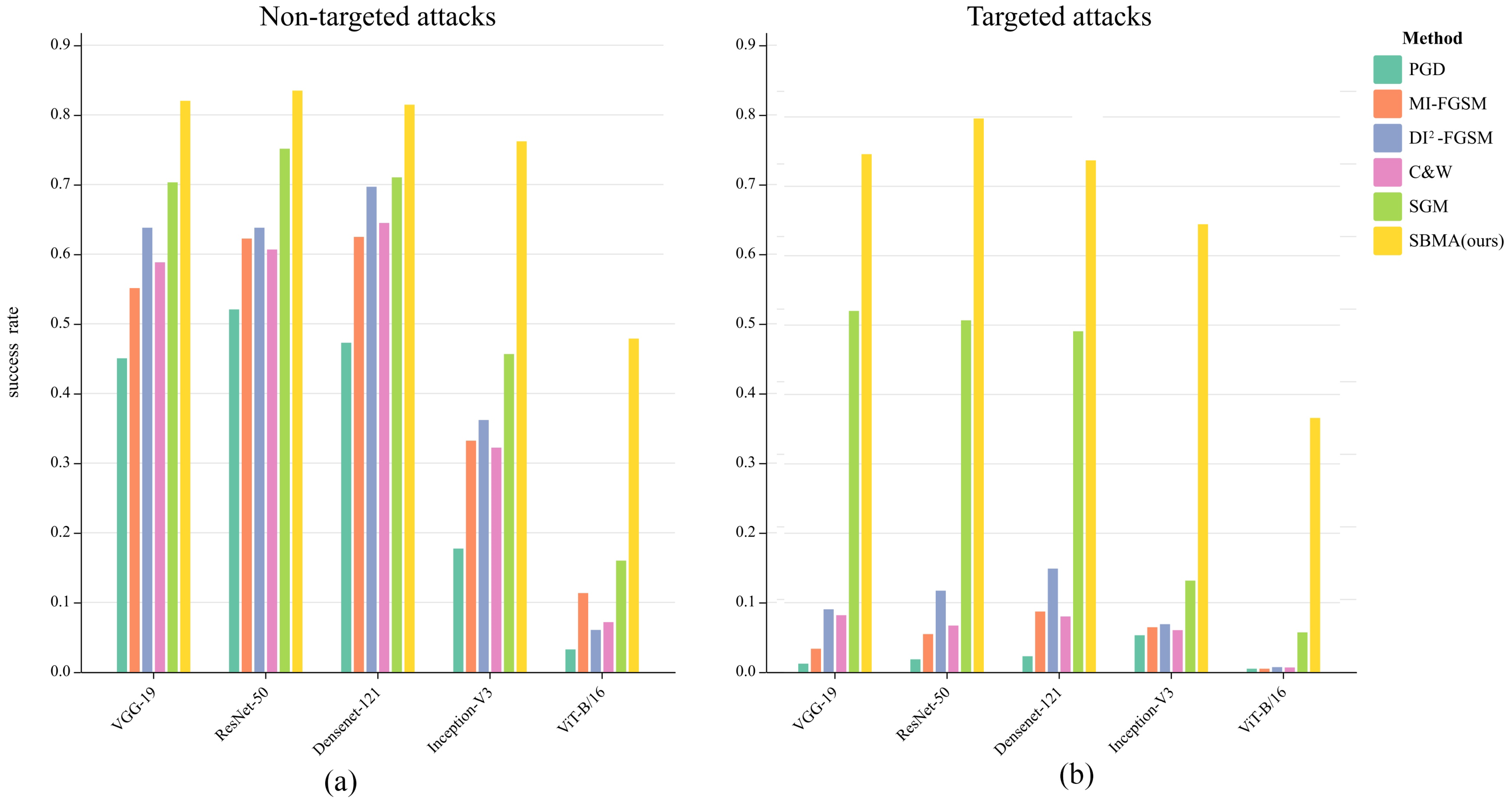
4.2.1. Attack Target Model Experiments

As shown in Table 1 and Table 2, while attacking the normal model, the transferability of the traditional methods was relatively low when either non-targeted or targeted attacks were performed. Considering especially CNN network structures (VGG-19, ResNet-50, DenseNet-121, and Inception-V3) compared to the vision transformer network structure (ViT-B/16), in the case of PGD non-targeted attacks, for example, the transferability dropped from a maximum of 45.05% to 3.25%. Fortunately, our SBMA method achieved the highest attack success rate compared to other methods and exhibited good transferability.

Table 1. Non-targeted attack experiments against normal models. The dataset used was Image-Net-1K, and the best results are in bold.

Surrogate Model	Attack Method	VGG-19	ResNet-50	DenseNet-121	Inception-V3	ViT-B/16
ResNet-18	PGD [9]	45.05%	52.07%	47.28%	17.73%	3.25%
	MI-FGSM [8]	55.13%	62.24%	62.48%	33.22%	11.34%
	${\mathrm{DI}}^2$-FGSM [10]	63.80%	63.80%	69.68%	36.19%	6.05%
	C&W [13]	58.83%	60.67%	64.48%	32.22%	7.17%
	SGM [50]	70.31%	75.14%	71.03%	45.66%	16.00%
	SBMA (ours)	82.02%	83.48%	81.46%	76.20%	47.88%

Table 2. Targeted attack experiments against normal models. The dataset used was Image-Net-1K, and the best results are in bold.

Surrogate Model	Attack Method	VGG-19	ResNet-50	DenseNet-121	Inception-V3	ViT-B/16
ResNet-18	PGD [9]	1.21%	1.84%	2.28%	5.30%	0.48%
	MI-FGSM [8]	3.36%	5.47%	8.72%	6.46%	0.48%
	${\mathrm{DI}}^2$-FGSM [10]	9.04%	11.73%	14.91%	6.90%	0.71%
	C&W [13]	8.19%	6.70%	8.01%	6.04%	0.66%
	SGM [50]	52.04%	50.69%	49.11%	13.18%	5.72%
	SBMA (ours)	74.63%	79.77%	73.10%	64.54%	36.62%

From Figure 3, we can see more intuitively that the transferability of the traditional methods decreased significantly when transforming from non-targeted attacks (subfigure (a)) to targeted attacks (subfigure (b)), while our SBMA method could still maintain a high transferability. This indicated that network models with different structures had a significant impact on the methods guided by the decision boundaries of the classifiers but had less impact on the methods guided by the sample probability distributions.

Figure 3. Comparison of success rates when attacking normal models. Subfigure (a) represents non-targeted attacks, and subfigure (b) represents targeted attacks.

Table 3 and Figure 4 present comparisons of the attacks on the normal model of DenseNet-121 and its robust models. From the results, we can see that, in terms of the success rate, the PGD method and the FGSM series methods almost failed when transferred to attack the robust models, and only the SGM method maintained a relatively high success rate. In contrast, our SBMA method maintained the highest success rate, although it also presented decreases in some indicators. This shows that our approach, guided by the probability distribution of the samples, was able to achieve high transferability by ignoring the negative effects of classifier robustness improvement, while the rest of the methods clearly failed in the face of the robustness model.

Table 3. Targeted attack experiments against the robust models of DenseNet-121 with ImageNet-1K dataset; the best results are in bold.

Surrogate Model	Attack Method	Normal	Adversarial Training	SIN	Augmix
ResNet-18	PGD [9]	2.28%	0.59%	1.26%	1.21%
	MI-FGSM [8]	8.72%	1.83%	4.71%	4.54%
	${\mathrm{DI}}^2$-FGSM [10]	14.91%	3.60%	8.40%	8.10%
	C&W [13]	8.01%	1.64%	4.23%	4.08%
	SGM [50]	49.11%	9.22%	28.53%	27.50%
	SBMA (ours)	73.10%	15.13%	60.27%	54.62%

Figure 4. Comparison of the success rates of targeted attacks on the robust models. Marked in red on the x-axis is the normal model of DenseNet-121, and the rest are the DenseNet-121 models that were trained by the robust methods.

4.2.2. Experiments on the CIFAR-100 Dataset

As shown in Table 4, when the dataset was replaced with CIFAR100 and targeted attacks were implemented, we obtained similar conclusions to those in Table 2, indicating that our method was still effective in the face of different datasets. However, we found that all metrics decreased to varying degrees when compared to the results under the ImageNet-1K dataset, as shown in Figure 5a. The CIFAR-100 dataset was divided into 100 classes, and the training set contained only 500 images with a size of 3 × 32 × 32 for each class, i.e., fewer in number and smaller in size compared to ImageNet-1K. Considering that the estimation of the sample probability distribution required a higher quality of samples, we input ImageNet-1K images of different sizes and different numbers to validate our suspicion. The results are shown in Table 5 and Figure 5b,c, where the higher the number of input images and the larger the size, the higher the attack success rate.

Table 4. Targeted attack experiments against normal models. The dataset used was CIFAR100, and the best results are in bold.

Surrogate Model	Attack Method	VGG-19	ResNet-50	DenseNet-121	Inception-V3	ViT-B/16
ResNet-18	PGD [9]	0.98%	1.56%	1.93%	4.49%	0.37%
	MI-FGSM [8]	2.84%	4.52%	7.39%	5.95%	0.40%
	${\mathrm{DI}}^2$-FGSM [10]	7.66%	9.94%	11.43%	5.85%	0.48%
	C&W [13]	6.93%	5.67%	6.78%	5.12%	0.56%
	SGM [50]	44.08%	40.80%	41.60%	11.16%	3.65%
	SBMA (ours)	52.68%	51.31%	49.38%	41.56%	20.85%

Figure 5. Subfigure (a) represents a comparison of the attack success rates of our SBMA method for different datasets. Subfigure (b) represents a comparison of the attack success rates using the ImageNet-1K dataset with an input image size of 3 × 224 × 224 and different numbers of images. Subfigure (c) represents a comparison of the attack success rates using the ImageNet-1K dataset with an input image number of 1300p and different sizes.

Table 5. Comparison results of input images of different sizes and different numbers under ImageNet-1K dataset. The surrogate model used was ResNet-18, and the target model was DenseNet-121.

Number of Samples with 3 × 224 × 224		Size of Samples with 1300p
1300p	73.10%	3 × 224 × 224	73.10%
650p	62.69%	3 × 112 × 112	67.52%
300p	45.16%	3 × 64 × 64	58.35%
100p	21.08%	3 × 32 × 32	40.44%

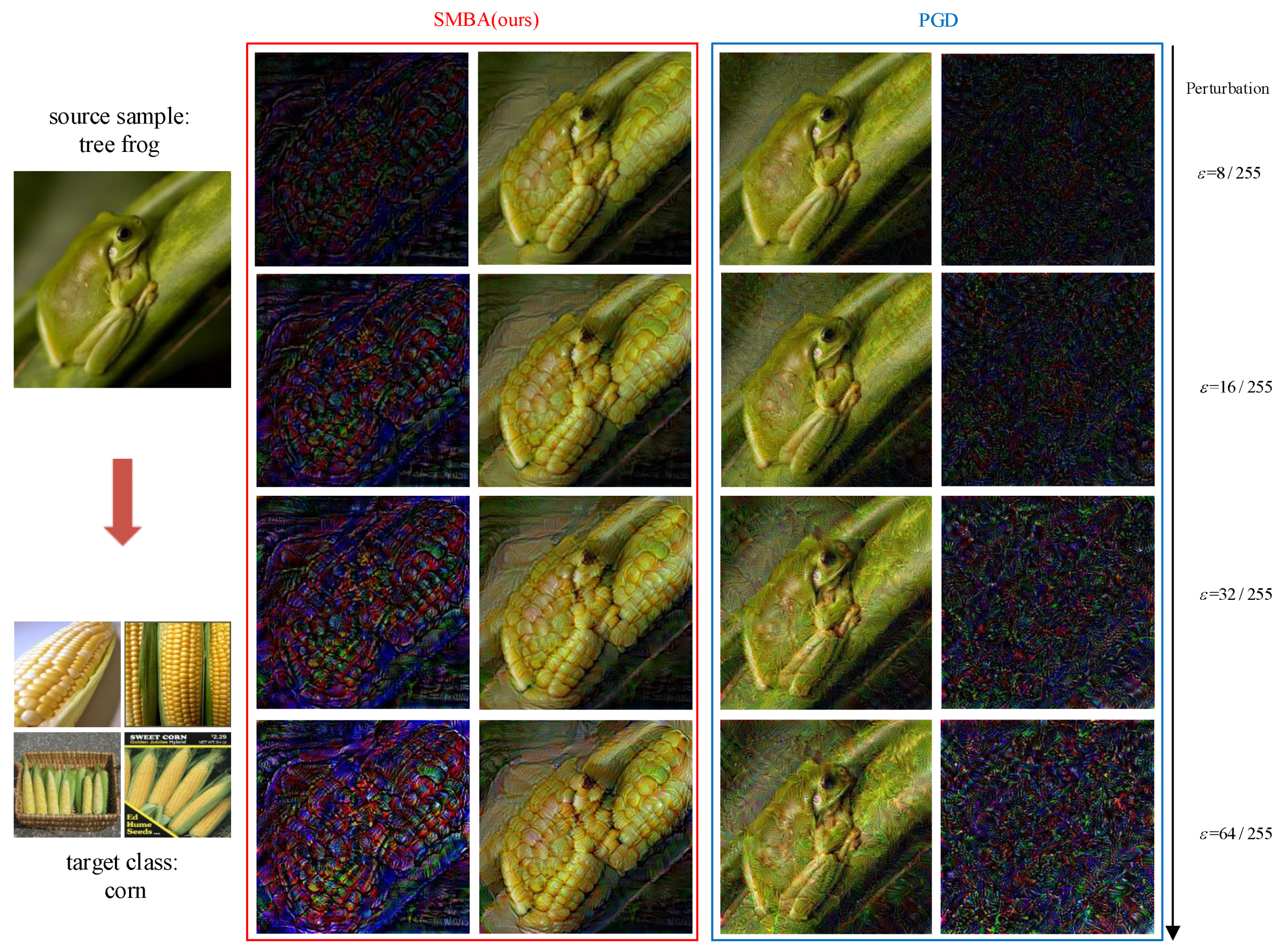
4.3. Visualization and Interpretability

In this section, the traditional PGD method is chosen for a visual comparison with our SMBA method, which is illustrated from the perspectives of both generating adversarial samples and the corresponding feature space.

4.3.1. Generating Adversarial Samples

We appropriately increased the perturbation strength and observed the adversarial sample images and their perturbations generated by different methods from the perspective of targeted attacks. As shown in Figure 6 and Figure 7, the perturbations generated by the PGD method were irregular, while the SMBA method clearly transferred the tree frog (source sample) toward the semantic features of vine snake and corn (target classes), and the generated perturbation had the semantic feature form of the target class. This showed that our method was indeed able to learn the semantic features of the target class.

Figure 6. Example 1 of adversarial sample generation for targeted attacks. The source sample is a tree frog, and the target class is a vine snake. The 1st and 2nd columns represent the perturbations (3 times the pixel difference between the adversarial sample and the source sample) and the images of the adversarial samples generated by our SMBA methods. The 3rd and 4th columns represent the same content generated by the PGD methods. The perturbation intensity increases from top to bottom.

Figure 7. Example 2 of adversarial sample generation for targeted attacks. The source sample is a tree frog, and the target class is corn.

To further demonstrate the reliability of our SMBA method, we set the source samples as pure gray images and the target classes as multi-classes, as shown in Figure 8. Obviously, the adversarial samples generated by the PGD method were irregularly noisy, while the adversarial samples generated by our SMBA method could still learn the semantic features of the target classes clearly.

Figure 8. Perturbation imaging of targeted attacks. The source sample is a pure gray image with a pixel size of 0.5, the 1st row indicates multiple target classes, and the 2nd and 3rd rows indicate the images of the adversarial samples generated by different methods.

4.3.2. Corresponding Feature Space

In the non-targeted attacks, we visualized the two-dimensional feature space distribution patterns of the source sample and the adversarial sample. As shown in Figure 9, when the adversarial samples generated by the non-targeted attacks on the surrogate model (ResNet-18) transferred to attack the target model (DenseNet-121), the black dashed circle area of subfigure (a) showed a mixed state, which meant that the adversarial samples generated by the PGD method were not completely removed from the feature space of the source samples. Conversely, the adversarial samples generated by the SMBA method were completely removed from the feature space of the source samples along the black arrow of subfigure (b). This indicated that our method could completely remove the adversarial samples from the original probability distribution space to enhance the transferability when performing non-targeted attacks.

Figure 9. Comparison of the transferability of the adversarial samples generated by non-targeted attacks. We used the adversarial samples generated by non-targeted attacks on the surrogate model (ResNet-18) to transfer to attack the target model (DenseNet-121). Subfigure (a) represents the two-dimensional feature space distribution patterns of the source samples and the adversarial samples generated by our SMBA method, subfigure (b) represents the same content generated by the PGD method, and the attack intensity is $\epsilon =16/255$.

In the targeted attacks, we visualized the wandering paths of the individual adversarial samples generated by different methods in the feature space. As shown in Figure 10, when the perturbation strength increased, for the surrogate model in subfigure (a), the adversarial samples generated by different methods gradually moved out of the feature space of the source class and wandered toward and into the feature space of the target class; finally, the attacks were successful. For the target model in subfigure (b), the adversarial samples generated by the PGD method could not move out of the feature space of the source class (blue ➀ to ➆) and could not cross the decision boundary of the target model; thus, the transferable attacks failed. Fortunately, the adversarial samples generated by the SMBA method could still move out of the feature space of the source class and move towards and into the feature space of the target class. The pink dashed circle in subfigure (b) indicates the successful transferable attacks (red ➄ to ➆), which corresponds to the images with ‘✔’ marks in row (c), and we can see that the tree frog (source sample) gradually acquired the semantic feature form of the corn (target class). This indicated that our method could completely remove the adversarial sample from the original probability distribution space and cause them to wander toward and into the probability distribution space of the target class when conducting the targeted attacks; thus, the success rate of transferability was higher.

Figure 10. Comparison of the transferability of the adversarial samples generated by targeted attacks. With the perturbation strength increasing, subfigures (a,b) represent the wandering paths (7 steps from ➀ to ➆) in the two-dimensional feature space of the adversarial samples generated by different methods attacking the surrogate model (ResNet-18) and the target model (DenseNet-121). Rows (c,d) represent the images of the adversarial samples generated by different methods under different perturbation strengths. The images in subfigure (b) with the pink dashed circle indicate the successful transferable attacks, and their corresponding images are the images with ‘✔’ marks in row (c).

5. Conclusions

In this paper, we overcame the limitations of traditional adversarial sample generation methods based on the decision boundary guidance of classifiers and reinterpreted the generation mechanism of adversarial samples from the perspective of sample probability distribution.

Firstly, we found that if the adversarial samples were directed to move from the space of the original probability distributions to the space of the target probability distributions, the adversarial samples could learn the semantic features of the target samples, which could significantly boost the transferability and interpretability when faced with classifiers of different structures.

Secondly, we proved that classification models could be transformed into energy-based models according to the logits layer of classification models, so that we could use the SM series methods to estimate the probability density of samples.

Therefore, we proposed a probability-distribution-guided SMBA method that used the SM series methods to align the gradient of the classifiers with the samples after transforming the classification models into energy-based models, so that the gradient of the classifier could be used to move the adversarial samples out of the original probability distribution and wander toward and into the target probability distribution.

Extensive experiments demonstrated that our method showed good performance in terms of transferability when faced with different datasets and models and could provide a reasonable explanation from the perspective of mathematical theory and feature space. Meanwhile, our findings also established a bridge between probabilistic generative models and adversarial samples, providing a new entry angle for research into adversarial samples and bringing new thinking to AI security.

References

1. Akhtar, N.; Mian, A. Threat of adversarial attacks on deep learning in computer vision: A survey. IEEE Access 2018, 6, 14410–14430. [Google Scholar] [CrossRef]
2. Szegedy, C.; Zaremba, W.; Sutskever, I.; Bruna, J.; Erhan, D.; Goodfellow, I.; Fergus, R. Intriguing properties of neural networks. arXiv 2013, arXiv:1312.6199. [Google Scholar]
3. Duan, R.; Ma, X.; Wang, Y.; Bailey, J.; Qin, A.K.; Yang, Y. Adversarial camouflage: Hiding physical-world attacks with natural styles. In Proceedings of the IEEE/CVF Conference on Computer Vision and Pattern Recognition, Seattle, WA, USA, 13–19 June 2020; pp. 1000–1008. [Google Scholar]
4. Zhang, Y.; Gong, Z.; Zhang, Y.; Bin, K.; Li, Y.; Qi, J.; Wen, H.; Zhong, P. Boosting transferability of physical attack against detectors by redistributing separable attention. Pattern Recognit. 2023, 138, 109435. [Google Scholar] [CrossRef]
5. Welling, M.; Teh, Y.W. Bayesian learning via stochastic gradient Langevin dynamics. In Proceedings of the 28th International Conference on Machine Learning (ICML-11), Washington, DC, USA, 28 June–2 July 2011; pp. 681–688. [Google Scholar]
6. Goodfellow, I.J.; Shlens, J.; Szegedy, C. Explaining and harnessing adversarial examples. arXiv 2014, arXiv:1412.6572. [Google Scholar]
7. Kurakin, A.; Goodfellow, I.J.; Bengio, S. Adversarial examples in the physical world. In Artificial Intelligence Safety and Security; Chapman and Hall/CRC: Boca Raton, FL, USA, 2018; pp. 99–112. [Google Scholar]
8. Dong, Y.; Liao, F.; Pang, T.; Su, H.; Zhu, J.; Hu, X.; Li, J. Boosting adversarial attacks with momentum. In Proceedings of the IEEE Conference on Computer Vision and Pattern Recognition, Salt Lake City, UT, USA, 18–23 June 2018; pp. 9185–9193. [Google Scholar]
9. Madry, A.; Makelov, A.; Schmidt, L.; Tsipras, D.; Vladu, A. Towards deep learning models resistant to adversarial attacks. arXiv 2017, arXiv:1706.06083. [Google Scholar]
10. Xie, C.; Zhang, Z.; Zhou, Y.; Bai, S.; Wang, J.; Ren, Z.; Yuille, A.L. Improving transferability of adversarial examples with input diversity. In Proceedings of the IEEE/CVF Conference on Computer Vision and Pattern Recognition, Long Beach, CA, USA, 15–20 June 2019; pp. 2730–2739. [Google Scholar]
11. Papernot, N.; McDaniel, P.; Jha, S.; Fredrikson, M.; Celik, Z.B.; Swami, A. The limitations of deep learning in adversarial settings. In Proceedings of the 2016 IEEE European Symposium on Security and Privacy (EuroS&P), Saarbrucken, Germany, 21–24 March 2016; pp. 372–387. [Google Scholar]
12. Simonyan, K.; Vedaldi, A.; Zisserman, A. Deep inside convolutional networks: Visualising image classification models and saliency maps. arXiv 2013, arXiv:1312.6034. [Google Scholar]
13. Carlini, N.; Wagner, D. Towards evaluating the robustness of neural networks. In Proceedings of the 2017 IEEE Symposium on Security and Privacy (SP), San Jose, CA, USA, 22–26 May 2017; pp. 39–57. [Google Scholar]
14. Su, J.; Vargas, D.V.; Sakurai, K. One pixel attack for fooling deep neural networks. IEEE Trans. Evol. Comput. 2019, 23, 828–841. [Google Scholar] [CrossRef] [Green Version]
15. Papernot, N.; McDaniel, P.; Goodfellow, I.; Jha, S.; Celik, Z.B.; Swami, A. Practical black-box attacks against machine learning. In Proceedings of the 2017 ACM on Asia Conference on Computer and Communications Security, Abu Dhabi, United Arab Emirates, 2–6 April 2017; pp. 506–519. [Google Scholar]
16. Pengcheng, L.; Yi, J.; Zhang, L. Query-efficient black-box attack by active learning. In Proceedings of the 2018 IEEE International Conference on Data Mining (ICDM), Singapore, 17–20 November 2018; pp. 1200–1205. [Google Scholar]
17. Wu, W.; Su, Y.; Chen, X.; Zhao, S.; King, I.; Lyu, M.R.; Tai, Y.W. Boosting the transferability of adversarial samples via attention. In Proceedings of the IEEE/CVF Conference on Computer Vision and Pattern Recognition, Seattle, WA, USA, 13–19 June 2020; pp. 1161–1170. [Google Scholar]
18. Li, Y.; Bai, S.; Zhou, Y.; Xie, C.; Zhang, Z.; Yuille, A. Learning transferable adversarial examples via ghost networks. In Proceedings of the AAAI Conference on Artificial Intelligence, New York, NY, USA, 7–12 February 2020; Volume 34, pp. 11458–11465. [Google Scholar]
19. Hu, Z.; Li, H.; Yuan, L.; Cheng, Z.; Yuan, W.; Zhu, M. Model scheduling and sample selection for ensemble adversarial example attacks. Pattern Recognit. 2022, 130, 108824. [Google Scholar] [CrossRef]
20. Dong, Y.; Su, H.; Wu, B.; Li, Z.; Liu, W.; Zhang, T.; Zhu, J. Efficient decision-based black-box adversarial attacks on face recognition. In Proceedings of the IEEE/CVF Conference on Computer Vision and Pattern Recognition, Long Beach, CA, USA, 15–20 June 2019; pp. 7714–7722. [Google Scholar]
21. Hansen, N.; Ostermeier, A. Completely derandomized self-adaptation in evolution strategies. Evol. Comput. 2001, 9, 159–195. [Google Scholar] [CrossRef]
22. Brunner, T.; Diehl, F.; Le, M.T.; Knoll, A. Guessing smart: Biased sampling for efficient black-box adversarial attacks. In Proceedings of the IEEE/CVF International Conference on Computer Vision, Seoul, Republic of Korea, 27 October–2 November 2019; pp. 4958–4966. [Google Scholar]
23. Shi, Y.; Han, Y.; Tian, Q. Polishing decision-based adversarial noise with a customized sampling. In Proceedings of the IEEE/CVF Conference on Computer Vision and Pattern Recognition, Seattle, WA, USA, 13–19 June 2020; pp. 1030–1038. [Google Scholar]
24. Rahmati, A.; Moosavi-Dezfooli, S.M.; Frossard, P.; Dai, H. Geoda: A geometric framework for black-box adversarial attacks. In Proceedings of the IEEE/CVF Conference on Computer Vision and Pattern Recognition, Seattle, WA, USA, 13–19 June 2020; pp. 8446–8455. [Google Scholar]
25. Goodfellow, I.; Pouget-Abadie, J.; Mirza, M.; Xu, B.; Warde-Farley, D.; Ozair, S.; Courville, A.; Bengio, Y. Generative adversarial networks. Commun. ACM 2020, 63, 139–144. [Google Scholar] [CrossRef]
26. Xiao, C.; Li, B.; Zhu, J.Y.; He, W.; Liu, M.; Song, D. Generating adversarial examples with adversarial networks. arXiv 2018, arXiv:1801.02610. [Google Scholar]
27. Jandial, S.; Mangla, P.; Varshney, S.; Balasubramanian, V. Advgan++: Harnessing latent layers for adversary generation. In Proceedings of the IEEE/CVF International Conference on Computer Vision Workshops, Seoul, Republic of Korea, 27 October–2 November 2019. [Google Scholar]
28. Moosavi-Dezfooli, S.M.; Fawzi, A.; Frossard, P. Deepfool: A simple and accurate method to fool deep neural networks. In Proceedings of the IEEE Conference on Computer Vision and Pattern Recognition, Las Vegas, NV, USA, 27–30 June 2016; pp. 2574–2582. [Google Scholar]
29. Moosavi-Dezfooli, S.M.; Fawzi, A.; Fawzi, O.; Frossard, P. Universal adversarial perturbations. In Proceedings of the IEEE Conference on Computer Vision and Pattern Recognition, Honolulu, HI, USA, 21–26 July 2017; pp. 1765–1773. [Google Scholar]
30. Zhou, B.; Khosla, A.; Lapedriza, A.; Oliva, A.; Torralba, A. Learning deep features for discriminative localization. In Proceedings of the IEEE Conference on Computer Vision and Pattern Recognition, Las Vegas, NV, USA, 27–30 June 2016; pp. 2921–2929. [Google Scholar]
31. Vadillo, J.; Santana, R.; Lozano, J.A. Extending adversarial attacks to produce adversarial class probability distributions. arXiv 2023, arXiv:2004.06383. [Google Scholar]
32. Joyce, J.M. Kullback-leibler divergence. In International Encyclopedia of Statistical Science; Springer: Berlin/Heidelberg, Germany, 2011; pp. 720–722. [Google Scholar]
33. Wang, X.; Zhai, C.; Roth, D. Understanding evolution of research themes: A probabilistic generative model for citations. In Proceedings of the 19th ACM SIGKDD International Conference on Knowledge Discovery and Data Mining, Chicago, IL, USA, 11–14 August 2013; pp. 1115–1123. [Google Scholar]
34. Alain, G.; Bengio, Y.; Yao, L.; Yosinski, J.; Thibodeau-Laufer, E.; Zhang, S.; Vincent, P. GSNs: Generative stochastic networks. Inf. Inference J. IMA 2016, 5, 210–249. [Google Scholar] [CrossRef] [Green Version]
35. Taketo, M.; Schroeder, A.C.; Mobraaten, L.E.; Gunning, K.B.; Hanten, G.; Fox, R.R.; Roderick, T.H.; Stewart, C.L.; Lilly, F.; Hansen, C.T. FVB/N: An inbred mouse strain preferable for transgenic analyses. Proc. Natl. Acad. Sci. USA 1991, 88, 2065–2069. [Google Scholar] [CrossRef] [PubMed]
36. Germain, M.; Gregor, K.; Murray, I.; Larochelle, H. Made: Masked autoencoder for distribution estimation. In Proceedings of the International Conference on Machine Learning, Lille, France, 6–11 July 2015; pp. 881–889. [Google Scholar]
37. Van den Oord, A.; Kalchbrenner, N.; Espeholt, L.; Vinyals, O.; Graves, A.; Kavukcuoglu, K. Conditional image generation with pixelcnn decoders. Adv. Neural Inf. Process. Syst. 2016, 29, 1–13. [Google Scholar]
38. An, J.; Cho, S. Variational autoencoder based anomaly detection using reconstruction probability. Spec. Lect. IE 2015, 2, 1–18. [Google Scholar]
39. Llorente, F.; Curbelo, E.; Martino, L.; Elvira, V.; Delgado, D. MCMC-driven importance samplers. Appl. Math. Model. 2022, 111, 310–331. [Google Scholar] [CrossRef]
40. Du, Y.; Mordatch, I. Implicit generation and modeling with energy based models. Adv. Neural Inf. Process. Syst. 2019, 32, 1–11. [Google Scholar]
41. Hinton, G.E. A practical guide to training restricted Boltzmann machines. In Neural Networks: Tricks of the Trade: Second Edition; Springer: Berlin/Heidelberg, Germany, 2012; pp. 599–619. [Google Scholar]
42. Hinton, G.E.; Osindero, S.; Teh, Y.W. A fast learning algorithm for deep belief nets. Neural Comput. 2006, 18, 1527–1554. [Google Scholar] [CrossRef]
43. Ho, J.; Jain, A.; Abbeel, P. Denoising diffusion probabilistic models. Adv. Neural Inf. Process. Syst. 2020, 33, 6840–6851. [Google Scholar]
44. Hyvärinen, A.; Dayan, P. Estimation of non-normalized statistical models by score matching. J. Mach. Learn. Res. 2005, 6, 695–709. [Google Scholar]
45. Song, Y.; Garg, S.; Shi, J.; Ermon, S. Sliced score matching: A scalable approach to density and score estimation. In Proceedings of the Uncertainty in Artificial Intelligence, Virtual, 3–6 August 2020; pp. 574–584. [Google Scholar]
46. Grathwohl, W.; Wang, K.C.; Jacobsen, J.H.; Duvenaud, D.; Norouzi, M.; Swersky, K. Your classifier is secretly an energy based model and you should treat it like one. arXiv 2019, arXiv:1912.03263. [Google Scholar]
47. Deng, J.; Dong, W.; Socher, R.; Li, L.J.; Li, K.; Fei-Fei, L. Imagenet: A large-scale hierarchical image database. In Proceedings of the 2009 IEEE Conference on Computer Vision and Pattern Recognition, Miami, FL, USA, 20–25 June 2009; pp. 248–255. [Google Scholar]
48. He, K.; Zhang, X.; Ren, S.; Sun, J. Deep residual learning for image recognition. In Proceedings of the IEEE Conference on Computer Vision and Pattern Recognition, Las Vegas, NV, USA, 27–30 June 2016; pp. 770–778. [Google Scholar]
49. Ruder, S. An overview of gradient descent optimization algorithms. arXiv 2016, arXiv:1609.04747. [Google Scholar]
50. Wu, D.; Wang, Y.; Xia, S.T.; Bailey, J.; Ma, X. Skip connections matter: On the transferability of adversarial examples generated with resnets. arXiv 2020, arXiv:2002.05990. [Google Scholar]
51. Simonyan, K.; Zisserman, A. Very deep convolutional networks for large-scale image recognition. arXiv 2014, arXiv:1409.1556. [Google Scholar]
52. Huang, G.; Liu, Z.; Van Der Maaten, L.; Weinberger, K.Q. Densely connected convolutional networks. In Proceedings of the IEEE Conference on Computer Vision and Pattern Recognition, Honolulu, HI, USA, 21–26 July 2017; pp. 4700–4708. [Google Scholar]
53. Szegedy, C.; Ioffe, S.; Vanhoucke, V.; Alemi, A. Inception-v4, inception-resnet and the impact of residual connections on learning. In Proceedings of the AAAI Conference on Artificial Intelligence, San Francisco, CA, USA, 4–9 February 2017; Volume 31. [Google Scholar]
54. Dosovitskiy, A.; Beyer, L.; Kolesnikov, A.; Weissenborn, D.; Zhai, X.; Unterthiner, T.; Dehghani, M.; Minderer, M.; Heigold, G.; Gelly, S.; et al. An image is worth 16x16 words: Transformers for image recognition at scale. arXiv 2020, arXiv:2010.11929. [Google Scholar]
55. Salman, H.; Ilyas, A.; Engstrom, L.; Kapoor, A.; Madry, A. Do adversarially robust imagenet models transfer better? Adv. Neural Inf. Process. Syst. 2020, 33, 3533–3545. [Google Scholar]
56. Geirhos, R.; Rubisch, P.; Michaelis, C.; Bethge, M.; Wichmann, F.A.; Brendel, W. ImageNet-trained CNNs are biased towards texture; increasing shape bias improves accuracy and robustness. arXiv 2018, arXiv:1811.12231. [Google Scholar]
57. Hendrycks, D.; Mu, N.; Cubuk, E.D.; Zoph, B.; Gilmer, J.; Lakshminarayanan, B. Augmix: A simple method to improve robustness and uncertainty under data shift. In Proceedings of the International Conference on Learning Representations, Addis Ababa, Ethiopia, 26–30 April 2020; Volume 1, p. 6. [Google Scholar]
58. Krizhevsky, A.; Hinton, G. Learning Multiple Layers of Features from Tiny Images; Technical Report; University of Toronto: Toronto, ON, Canada, 2009. [Google Scholar]
59. Shlens, J. A tutorial on principal component analysis. arXiv 2014, arXiv:1404.1100. [Google Scholar]