Article

Assessing Multinomial Distributions with a Bayesian Approach

1
Department of Mathematical & Computational Sciences, University of Toronto Mississauga, Toronto, ON L5L 1C6, Canada
2
Department of Mathematics & Statistics, McMaster University, 1280 Main Street West, Hamilton, ON L8S 4L8, Canada
*
Author to whom correspondence should be addressed.
Mathematics 2023, 11(13), 3007; https://doi.org/10.3390/math11133007
Submission received: 10 June 2023 / Revised: 2 July 2023 / Accepted: 4 July 2023 / Published: 6 July 2023
(This article belongs to the Special Issue Research Progress and Application of Bayesian Statistics)

Abstract

:
This paper introduces a unified Bayesian approach for testing various hypotheses related to multinomial distributions. The method calculates the Kullback–Leibler divergence between two specified multinomial distributions, followed by comparing the change in distance from the prior to the posterior through the relative belief ratio. A prior elicitation algorithm is used to specify the prior distributions. To demonstrate the effectiveness and practical application of this approach, it has been applied to several examples.

1. Introduction

Multinomial distribution tests are a crucial statistical tool in many fields, especially when data can be categorized into multiple groups. These tests were first proposed by Karl Pearson in 1890 and have since been widely used to analyze and make inferences about the probabilities or proportions associated with each category in the multinomial distribution [1].
Let the sample space A of a random experiment be the union of a finite number k of mutually disjoint sets (categories) A 1 , , A k . Assume that P ( A j ) = θ j , j = 1 , , k , where j = 1 k θ j = 1 . Here θ j represents the probability that the outcome is an element of the set A j . The random experiment is to be repeated n independent times. Define the random variables Y j to be the number of times the outcome is an element of set A j , j = 1 , , k . That is, Y 1 , , Y k = n Y 1 Y 2 Y k 1 denote the frequencies with which the outcome belongs to A 1 , , A k , respectively. Then the joint probability mass function (pmf) of Y 1 , , Y k is the multinomial with parameters n , θ 1 , , θ k  [2]. It is desired to test the null hypothesis:
H 0 1 : θ j = θ j 0 ,   for   j = 1 , , k
against all alternatives, where θ j 0 are known constants. Within the classical frequentist framework, to test H 0 1 , it is common to use the test statistic [3]:
χ 2 = j = 1 k ( Y j n θ j 0 ) 2 n θ j 0 .
It is known that, under H 0 1 , the limiting distribution of χ 2 is chi-squared with k 1 degrees of freedom. When H 0 1 is true, n θ j 0 represents the expected value of Y j . This implies the observed value χ 2 should not be too large if H 0 1 is true. For a given significance level α , an approximate test of size α is to reject H 0 1 if the observed χ 2 > χ k 1 2 ( α ) , where the χ k 1 2 ( α ) is the 1 α quantile of the chi-squared distribution with k 1 degrees of freedom; otherwise, fail to reject H 0 1 . Other possible tests for H 0 1 include Fisher’s exact test and likelihood ratio tests [4].
If there are r independent samples, then the interest is to test whether the r samples come from the same multinomial population or that r multinomial populations are different. Let A 1 , A 2 , , A k denote k possible types of categories in the ith sample, i = 1 , , k . Let the probability that an outcome of category A j will occur for the ith population (or ith sample) be denoted by θ j | i . Note that, j = 1 k θ j | i = 1 for each i = 1 , , r . Moreover, let Y j | i be the number of times the outcome is an element of A j in sample i. Consider the completely specified hypothesis:
H 0 2 : θ j | i = θ j 0 | i ,   for   j = 1 , 2 , , k .
Under H 0 2 , the test statistic in (2) can be extended to
χ 2 = i = 1 r χ i 2 = i = 1 r j = 1 k ( Y j | i n i θ j 0 | i ) 2 n i θ j 0 | i .
If H 0 2 is true, then χ 2 in (4) has an approximately chi-squared distribution with r ( k 1 ) degrees of freedom. Likewise, for a given significance level α , an approximate test of size α is to reject H 0 2 if the observed χ 2 is bigger than χ r ( k 1 ) 2 ( α ) ; otherwise, fail to reject H 0 2  [5].
A third and more common hypothesis is to test whether the r multinomial populations are the same without specifying the values of the θ j | i . That is, we consider the null hypothesis:
H 0 3 : θ j | 1 = θ j | 2 = = θ j | r = θ j ,   for   j = 1 , 2 , , k .
The test statistics to test H 0 3 are given by
χ 2 = i = 1 r χ i 2 = i = 1 r j = 1 k ( Y j | i n i θ ^ j | i ) 2 n i θ ^ j | i ,
where θ ^ j | i = i = 1 r Y j | i i = 1 r n i = i = 1 r Y j | i n . Here, n i denotes the sample size of sample i and i = 1 r Y j | i represents the total in category A j . Note that θ ^ j | i represents the pooled maximum likelihood estimator (MLE) of θ j under H 0 3 . It is known that the limiting distribution of χ 2 in (6) is a chi-squared distribution with ( r 1 ) ( k 1 ) degrees of freedom. So, for a given significance level α , an approximate test of size α is to reject H 0 3 if the observed χ 2 > χ ( r 1 ) ( k 1 ) 2 ( α ) ; otherwise, fail to reject H 0 3  [5]. It is worth mentioning that several other frequentist methods for testing the multinomial distribution have been proposed, utilizing different distance measures. These methods include the Euclidean distance proposed by [6], the smooth total variation distance introduced by [7], and ϕ -divergences discussed by [8]. These approaches provide alternative ways to assess the goodness-of-fit of the multinomial distribution using distance metrics.
Refs. [9,10,11,12,13] made early advances in Bayesian methods for analyzing categorical data, focusing on smoothing proportions in contingency tables and inference about odds ratios, respectively. These methods typically employed conjugate beta and Dirichlet priors. Ref. [14,15] extended these methods to develop Bayesian analogs of small-sample frequentist tests for 2 × 2 tables, also using such priors. Ref. [16] recommended the use of the uniform prior for predictive inference, but other priors were also suggested by discussants of his paper. The Jeffreys prior is the most commonly used prior for binomial inference, partially due to its invariance to the scale of measurement for the parameter. Reference priors (see [17]), such as the Jeffreys prior for the binomial parameter (see [18]), are viable options, but their specification can be computationally complex. Ref. [10] may have been the first to utilize an empirical Bayesian approach with contingency tables, estimating parameters in gamma and log-normal priors for association factors. Empirical Bayes involves estimating the prior distribution from the observed data itself and is particularly useful when dealing with large amounts of data. Refs. [19,20] derived integral expressions for the posterior distributions of the difference, ratio, and odds ratio under independent beta priors. Ref. [19] introduced Bayesian highest posterior density (HPD) confidence intervals for these measures. The HPD approach ensures that the posterior probability matches the desired confidence level, and the posterior density is higher inside the interval than outside. Ref. [21] discussed Bayesian confidence intervals for association parameters in 2 × 2 tables. They argued that to achieve good coverage performance in the frequentist sense across the entire parameter space, it is advisable to use relatively diffuse priors. Even uniform priors are often too informative, and they recommended the use of the Jeffreys prior. Bayesian methods for analyzing categorical data have been extensively surveyed in the literature, including comprehensive reviews by [22,23] with a focus on contingency table analysis. Refs. [24,25,26] proposed tests based on Bayesian nonparametric methods using Dirichlet process priors.
We build on the recent work of [27] by extending their Bayesian approach for hypothesis testing on one-sample proportions based on Kullback–Leibler divergence and relative belief ratio, using a uniform (0, 1) prior on binomial proportions, to multinomial distributions. Our goal is to provide a comprehensive Bayesian approach for testing hypotheses H 0 1 , H 0 2 , and H 0 3 . We derive distance formulas and use the Dirichlet distribution as a prior on probabilities. To ensure proper values of the prior’s hyperparameters, we employ the elicitation algorithm developed by [28]. The proposed approach offers several advantages, including computational simplicity, ease of interpretation, evidence in favor of the null hypothesis, and no requirement to specify a significance level.
The paper is structured as follows. Section 2 provides an overview of the relative belief ratio inference and KL divergence. Section 3 details the proposed approach, including the formulas and computational algorithms. In Section 4, several examples are presented to illustrate the approach. Finally, Section 5 contains concluding remarks and discussions.

2. Relevant Background

2.1. Inferences Using Relative Belief

Ref. [29] introduced the relative belief ratio, which has become a popular tool in statistical hypothesis testing theory. Several works have employed this approach, including [30,31,32,33,34,35].
Suppose we have a statistical model with a density function { f θ ( y ) : θ Θ } with respect to the Lebesgue measure on the parameter space Θ . Let π ( θ ) be a prior on Θ . After observing the data y , the posterior distribution of θ can be expressed as
π ( θ | y ) = f θ ( y ) π ( θ ) m ( y ) ,
where m ( y ) = Θ f θ ( y ) π ( θ ) d θ .
Assume that the goal is to draw inferences about the parameter θ . If the prior π ( · ) and the posterior π ( · | y ) are continuous at θ , then the relative belief ratio for a hypothesized value θ 0 of θ can be expressed as follows:
R B ( θ 0 | y ) = π ( θ 0 | y ) π ( θ 0 ) ,
the ratio of the posterior density to the prior density at θ 0 . In other words, R B ( θ 0 | y ) quantifies how the belief in θ 0 being the true value has changed from prior to posterior. It is worth noting that when π ( · ) and π ( · | y ) are discrete, the relative belief ratio is defined through limits, and further details can be found in [29].
The relative belief ratio R B ( θ 0 | y ) provides a measure of evidence for θ 0 being the true value. A value of R B ( θ 0 | y ) > 1 indicates evidence in favor of θ 0 being the true value, whereas R B ( θ 0 | y ) < 1 indicates evidence against θ 0 being the true value. If R B ( θ 0 | y ) = 1 , there is no evidence in either direction.
Once the relative belief ratio is calculated, it is important to determine the strength of the evidence in favor of or against H 0 : θ = θ 0 . A common way to quantify this is by computing the tail probability [29]:
S t r ( θ 0 | y ) = Π ( R B ( θ | y ) R B ( θ 0 | y ) | y ) = { θ Θ : R B ( θ | y ) R B ( θ 0 | y ) } π ( · | y ) d θ ,
where Π ( · | y ) in (7) is the posterior cumulative distribution function with posterior density π ( · | y ) . Therefore, equation (7) represents the posterior probability that the true value of θ has a relative belief ratio no greater than that of the hypothesized value θ 0 . When R B ( θ 0 | y ) < 1 , there is evidence against θ 0 . A small value of S t r ( θ 0 | y ) indicates a high posterior probability that the true value has a relative belief ratio greater than R B ( θ 0 | y ) , indicating strong evidence against θ 0 . Conversely, when R B ( θ 0 | y ) > 1 , there is evidence in favor of θ 0 . A large value of S t r ( θ 0 | y ) indicates a low posterior probability that the true value has a relative belief ratio greater than R B ( θ 0 | y ) , indicating strong evidence in favor of θ 0 . A small value of S t r ( θ 0 | y ) indicates weak evidence in favor of θ 0 .

2.2. KL Divergence

The KL divergence, also referred to as relative entropy, is a measure of dissimilarity between two probability distributions that quantifies how far apart they are from each other. It was introduced by Solomon Kullback and Richard Leibler in 1951. Let P and Q be two discrete cumulative distribution functions (cdf’s) on the same probability space φ , with corresponding probability mass functions (pmf’s) p and q (with respect to the counting measure). The KL divergence between p and q is given by:
d ( p , q ) = x φ p ( x ) log ( p ( x ) q ( x ) ) .
The KL divergence is always non-negative, and it attains its minimum value when p = q almost surely. This property makes it a useful tool in many areas of machine learning and information theory, such as hypothesis testing, model selection, and clustering. One interpretation of the KL divergence is that it measures how much information is lost when using Q to approximate P. It is worth noting that the KL divergence is not symmetric: d ( p , q ) and d ( q , p ) are generally not equal. Therefore, it is important to specify which distribution is the “true” or “target” distribution and which is the “approximating” or “predicted” distribution for some applications when using KL divergence in practice, as noted by [36].
The following lemma is essential to the proposed approach.
Lemma 1. 
Let p ( y 1 , y 2 , , y r ) = p 1 ( y 1 ) p 2 ( y 2 ) p r ( y r ) and q ( y 1 , y 2 , , y r ) = q 1 ( y 1 ) q 2 ( y 2 ) q r ( y r ) , where p i ( y i ) and q i ( y i ) are probability mass functions with supports y i = 1 , , n i , i = 1 , , r . Then
d ( p , q ) = i = 1 r d ( p i , q i ) .
Proof. 
We have
d ( p , q ) = y 1 = 0 n 1 y r = 0 n r p ( y 1 , y 2 , , y r ) log p ( y 1 , y 2 , , y r ) q ( y 1 , y 2 , , y r ) = y 1 = 0 n 1 y r = 0 n r p 1 ( y 1 ) p r ( y r ) log p 1 ( y 1 ) p r ( y r ) q 1 ( y 1 ) q r ( y r ) = y 1 = 0 n 1 y r = 0 n r p 1 ( y 1 ) p r ( y r ) [ log p 1 ( y 1 ) + + log p r ( y r ) log q 1 ( y 1 ) log q r ( y r ) ] = y 1 = 0 n 1 y r = 0 n r p 1 ( y 1 ) p r ( y r ) log p 1 ( y 1 ) + + y 1 = 0 n 1 y r = 0 n r p 1 ( y 1 ) p r ( y r ) log p r ( y r ) y 1 = 0 n 1 y r = 0 n r p 1 ( y 1 ) p r ( y r ) log q 1 ( y 1 ) y 1 = 0 n 1 y r = 0 n r p 1 ( y 1 ) p r ( y r ) log q r ( y r ) .
Since, for i = 1 , , r , y i = 1 n i p i ( y i ) = y i = 1 n i q i ( y i ) = 1 , we have
d ( p , q ) = y 1 = 0 n 1 p 1 ( y 1 ) log p 1 ( y 1 ) + + y r = 0 n r p r ( y r ) log p r ( y r ) y 1 = 0 n 1 p 1 ( y 1 ) log q 1 ( y 1 ) y r = 0 n r p r ( y r ) log q r ( y r ) = y 1 = 0 n 1 p 1 ( y 1 ) log p 1 ( y 1 ) q 1 ( y 1 ) + + y r = 0 n r p r ( y r ) log p r ( y r ) q r ( y r ) = d ( p 1 , q 1 ) + + d ( p r , q r ) .

3. The Approach

3.1. Bayesian One-Sample Multinomial

Let Y = ( Y 1 , , Y k ) m u l t i n o m i a l ( n , θ 1 , , θ k ) . The joint pmf of Y 1 , , Y k is given by
p ( y 1 , , y k ) = ( n y 1 , y 2 , , y k ) j = 1 k θ j y j ,
where ( n y 1 , y 2 , , y k ) = n ! y 1 ! y k ! , j = 1 k θ j = 1 , and j = 1 k y j = n .
To test the null hypothesis H 0 1 as defined in (1), we first compute the Kullback–Leibler (KL) divergence between p ( y 1 , , y k ) and the pmf under H 0 1 represented by
q ( y 1 , , y k ) = ( n y 1 , y 2 , , y k ) j = 1 k θ j 0 y i .
Here, θ j 0 denotes the null hypothesis value for θ j . The following proposition provides the formula for the KL divergence between p and q.
Proposition 1. 
Let p ( y 1 , , y k ) and q ( y 1 , , y k ) be two joint probability mass functions as defined in (8) and (9), respectively. We have,
d ( p , q ) = n j = 1 k [ θ j log ( θ j θ j 0 ) ] .
Proof. 
Let the support of Y j be 1 , 2 , , n j , j = 1 , , k . We have
d ( p , q ) = y 1 = 0 n 1 y k = 0 n k p ( y 1 , , y k ) log p ( y 1 , , y k ) q ( y 1 , , y k ) = y 1 = 0 n 1 y k = 0 n k p ( y 1 , , y k ) log ( n y 1 , y 2 , , y k ) j = 1 k θ j y j ( n y 1 , y 2 , , y k ) j = 1 k θ j 0 y j = y 1 = 0 n 1 y k = 0 n k p ( y 1 , , y k ) log j = 1 k [ θ j θ j 0 ] y j .
Using the properties of logarithmic function, we get
d ( p , q ) = y 1 = 0 n 1 y k = 0 n k p ( y 1 , , y k ) j = 1 k y j log [ θ j θ j 0 ] = y 1 = 0 n 1 y k = 0 n k p ( y 1 , , y k ) × y 1 × log [ θ 1 θ 01 ] + y 1 = 0 n 1 y k = 0 n k p ( y 1 , , y k ) × y k × [ θ k θ k 0 ] = E [ Y 1 ] × log [ θ 1 θ 01 ] + + E [ Y k ] × log [ θ k θ k 0 ] = j = 1 k E [ Y j ] log [ θ j θ j 0 ] .
Since the marginal probability mass function of Y j , j = 1 , , k , is the binomial with parameters n and θ j , we get
d ( p , q ) = j = 1 k n θ j log [ θ j θ j 0 ] = n j = 1 k [ θ j log ( θ j θ j 0 ) ] .
To connect the distance formula presented in Proposition 1 with the test statistic χ 2 in (2), we use the Taylor series expansion of the function f ( x ) = x log x x 0 about x 0 . This gives us
f ( x ) = ( x x 0 ) + 0.5 ( x x 0 ) 2 1 x 0 +
If H 0 1 is true and n is large, then we can approximate the distance d ( p , q ) as
d ( p , q ) n j = 1 k ( θ j θ j 0 ) + 0.5 n j = 1 k ( θ j θ j 0 ) 2 θ j 0 .
Since the probabilities sum to 1, the first term in (10) equals 0. The second term in (10) can be expressed as
0.5 j = 1 k ( n θ j n θ j 0 ) 2 n θ j 0 = 0.5 j = 1 k ( E ( Y j ) n θ j 0 ) 2 n θ j 0 .
This shows a direct connection between the KL divergence and χ 2 .
For the proposed Bayesian test, the probabilities θ 1 , , θ k are now random. The suggested prior for the joint probabilities ( θ 1 , , θ k ) is the Dirichlet distribution with parameters α 1 , α k . That is,
( θ 1 , θ 2 , , θ k ) Dirichlet ( α 1 , α 2 , , α k ) .
To elicit the prior, we use the elicitation algorithm developed by [28], which requires some domain knowledge to provide a lower bound for each θ i . For convenience, we have made this algorithm available on Shiny at the following link: https://bayesian-chi-square-test.shinyapps.io/DirichletprocessKyusonlim/ (accessed on 23 May 2023). For comparison purposes, we also considered the non-informative (uniform) prior, and Jeffreys prior; see Section 4. For the proposed Bayesian approach, when ( θ 1 , , θ k ) has the prior defined in (11), we put
D = n j = 1 k [ θ j log ( θ j θ j 0 ) ] .
We also have that the posterior distribution of ( θ 1 , , θ k ) given the observed data y = ( y 1 , , y k ) is Dirichlet ( α 1 + y 1 , α 2 + y 2 , , α k + y k ) . We write
D y = n j = 1 k [ θ j log ( θ j θ j 0 ) ] .
Note that,
E ( θ j | y ) = α j + y j j = 1 k ( α j + y j ) = α j + y j n + j = 1 k α j = n n + j = 1 k α j y j n + ( 1 n n + j = 1 k α j ) α j j = 1 k α j ,
which is a convex combination between the sample proportion (MLE) and the prior mean. As n , the weak law of large numbers ensures that E ( θ j | y ) converges in probability to the true value of θ j . Hence, if H 0 1 is true, then D y a . s . 0 . Conversely, if H 0 1 is false, then D y a . s . c , where c > 0 . Proposition 1 establishes that d ( p , q ) = 0 if and only if θ j = θ j 0 . Therefore, testing H 0 1 : θ j = θ j 0 is equivalent to testing d ( p , q ) = 0 . It follows that when H 0 1 is true, the distribution of D y should be more concentrated around 0 than that of D. So, the proposed test involves comparing the distributions of D and D y around 0 using the relative belief ratio:
R B D ( 0 | y ) = π D ( 0 | y ) π D ( 0 ) ,
where π D ( 0 ) and π D ( 0 | y ) represent the probability density functions of D and D y , respectively. If R B D ( 0 | y ) > 1 , it provides evidence in favor of H 0 (since the distribution of D y is more concentrated around 0 than that of D). If R B D ( 0 | y ) < 1 , there is evidence against H 0 1 (as the distribution of D y is less concentrated around 0 than that of D). Additionally, we compute the strength of evidence S t r D ( 0 | y ) = Π D ( R B ( d | y ) R B ( 0 | y ) | y ) , where Π D ( · | y ) is the cumulative distribution function of D y . As π D ( · | y ) and π D ( · ) in (14) have no closed forms, R B D ( 0 | y ) and S t r D ( 0 | y ) need to be approximated. The following Algorithm 1 summarizes the steps required to test H 0 1 .
Algorithm 1 RB test for H 0 1
(i)
Generate ( θ 1 , θ 2 , , θ k ) from Dirichlet ( α 1 , α 2 , , α k ) based on the algorithm of [28] and compute D as defined in (12).
(ii)
Repeat step (ii) to obtain a sample of r 1 values of D.
(iii)
Generate ( θ 1 , θ 2 , , θ k ) given the observed data y = ( y 1 , , y k ) from Dirichlet ( α 1 + y 1 , α 2 + y 2 , , α k + y k ) and compute D y as defined in (13).
(iv)
Repeat step (iii) to obtain a sample of r 2 values of D y .
(v)
Compute the relative belief ratio and the strength as follows:
(a)
Let L be a positive number. Let F ^ D denote the empirical cdf of D based on the prior sample in (3) and for i = 0 , , L , let d ^ i / L be the estimate of d i / L , the ( i / L ) -the prior quantile of D. Here d ^ 0 = 0 , and d ^ 1 is the largest value of D. Let F ^ D ( · | y ) denote the empirical cdf based on D y . For d [ d ^ i / L , d ^ ( i + 1 ) / L ) , estimate R B D ( d | y ) = π D ( d | y ) / π D ( d ) by
R B ^ D ( d | y ) = L { F ^ D ( d ^ ( i + 1 ) / L | y ) F ^ D ( d ^ i / L | y ) } ,
the ratio of the estimates of the posterior and prior contents of [ d ^ i / L , d ^ ( i + 1 ) / L ) . Thus, we estimate R B D ( 0 | y ) = π D ( 0 | y ) / π D ( 0 ) by R B ^ D ( 0 | y ) = L F ^ D ( d ^ p 0 | y ) where p 0 = i 0 / L and i 0 are chosen so that i 0 / L is not too small (typically i 0 / L 0.05 ) .
(b)
Estimate the strength Π D ( R B D ( d | y ) R B D ( 0 | y ) | y ) by the finite sum
{ i i 0 : R B ^ D ( d ^ i / L | y ) R B ^ D ( 0 | y ) } ( F ^ D ( d ^ ( i + 1 ) / L | y ) F ^ D ( d ^ i / L | y ) ) .
For fixed L , as r 1 , r 2 , then d ^ i / L converges almost surely to d i / L and (15) and (16) converge almost surely to R B D ( d | y ) and Π D ( R B D ( d | y ) R B D ( 0 | y ) | y ) , respectively. See [34] for the details.

3.2. Bayesian r-Sample Multinomial Test with a Completely Specified Null Hypothesis

Consider r independent samples Y 1 , Y 2 , , Y r where each Y i = ( Y 1 | i , , Y k | i ) follows a multinomial distribution with parameters n i and θ i = ( θ 1 | i , , θ k | i ) , where j = 1 k θ j | i = 1 for i = 1 , , r . Here, θ j | i denotes the probability of an outcome falling in category j for the ith sample, and Y j | i represents the number of times the outcome falls in category j in the ith sample. The null hypothesis to be tested is H 0 2 : θ j | i = θ j 0 | i for j = 1 , 2 , , k , where θ j 0 | i are known constants.
Let the joint distribution of Y 1 , Y 2 , , Y r be
p ( y 1 , y 2 , , y r ) = i = 1 r p ( y i ) = i = 1 r { ( n i y 1 | i , y 2 | i , , y k | i ) j = 1 k θ j | i y j | i } .
The proposed test is based on measuring the KL divergence between p and
q ( y 1 , y 2 , , y r ) = i = 1 r q ( y i ) = i = 1 r { ( n i y 1 | i , y 2 | i , , y k | i ) j = 1 k θ j 0 | i y j 0 | i } .
The following proposition provides the expression for the KL divergence between p and q. The proof follows directly from Lemma 1 and Proposition 1.
Proposition 2. 
Let p ( y 1 , y 2 , , y r ) and q ( y 1 , y 2 , , y r ) be the two joint probability mass functions as defined in (17) and (18), respectively. Then
d ( p , q ) = i = 1 r { n i j = 1 k [ θ j | i log ( θ j | i θ j 0 | i ) ] } .
Proposition 2 provides a connection between the KL divergence formula and the test statistic χ 2 in (6). Using a Taylor series expansion, we can approximate the distance d ( p , q ) as follows:
d ( p , q ) 0.5 i = 1 r j = 1 k ( n i θ j | i n i θ j 0 | i ) 2 n i θ j 0 | i = 0.5 i = 1 r j = 1 k ( E ( Y j | i ) n i θ j 0 | i ) 2 n i θ j 0 | i ,
which reveals a close connection to χ 2 .
For the proposed Bayesian test of H 0 2 , we adopt the prior ( θ 1 | i , , θ k | i ) Dirichlet ( α 1 | i , α 2 | i , , α k | i ) , and use the algorithm developed in [28] to elicit the hyperparameters α j | i for j = 1 , , k and i = 1 , , r . In this case, we define the divergence measure as
D = i = 1 r { n i j = 1 k [ θ j | i log ( θ j | i θ j 0 | i ) ] } ,
where θ j 0 | i is the hypothesized value of θ j | i under the null hypothesis.
The posterior distribution of ( θ 1 | i , , θ k | i ) given the observed data y i = ( y 1 | i , , y k | i ) is then Dirichlet ( α 1 | i + y 1 | i , α 2 | i + y 2 | i , , α k | i + y k | i ) . In this case, the divergence measure becomes
D y = i = 1 r { n i j = 1 k [ θ j | i log ( θ j | i θ j 0 | i ) ] } .
The following algorithm outlines the steps required to test H 0 2 using the proposed Bayesian test (Algorithm 2):
Algorithm 2 RB test for H 0 2
(i)
For i = 1 , , r , generate ( θ 1 | i , θ 2 | i , , θ k | i ) from Dirichlet ( α 1 | i , α 2 | i , , α k | i ) based on the algorithm of [28] and compute D as defined in (19).
(ii)
Repeat step (i) to obtain a sample of r 1 values of D.
(iii)
For i = 1 , , r , generate ( θ 1 | i , θ 2 | i , , θ k | i ) given the observed data y i = ( y 1 | i , , y k | i ) from Dirichlet ( α 1 | i + y 1 | i , α 2 | i + y 2 | i , , α k | i + y k | i ) and compute D y as defined in (20).
(iv)
Repeat step (iii) to obtain a sample of r 2 values of D y .
(v)
Compute the relative belief ratio and strength as described in Algorithm 1.

3.3. Bayesian Test for Homogeneity in r-Sample Multinomial Data

Consider r independent samples Y 1 , Y 2 , , Y r , where for i = 1 , , r , Y i = ( Y 1 | i , , Y k | i ) multinomial ( n i , θ 1 | i , , θ k | i ) with j = 1 k θ j | i = 1 . To test the null hypothesis H 0 3 as defined in (5), it is required to measure the KL divergence between p and q as defined in (17) and (18) with θ j 0 | i is replaced by θ j . This requirement is offered in the following proposition.
Proposition 3. 
Consider the probability mass functions p and q as defined in (17) and (18) with θ j 0 | i is replaced by θ j . Then
d ( p , q ) = i = 1 r { n i j = 1 k [ θ j | i log ( θ j | i θ j ) ] }
and
θ j = arg min θ j d ( p , q ) = i = 1 r n i θ j | i i = 1 r n i = i = 1 r n i θ j | i n .
Proof. 
(21) follows directly from Lemma 2 by setting θ j | i = θ j . To prove (22), we use we use Lagrange multiplier with the constraint j = 1 r θ j = 1 :
L = L ( θ j , λ ) = i = 1 r { n i j = 1 k [ θ j | i log ( θ j | i θ j ) ] } + λ ( j = 1 r θ j 1 ) .
Now,
L θ j = i = 1 r n i θ j | i θ j + λ , j = 1 , , k .
Setting L θ j = 0 gives
θ j = i = 1 r n i θ j | i λ , j = 1 , , k .
Summing over both sides and applying the constraint gives
λ = j = 1 k i = 1 r n i θ j | i = i = 1 r n i j = 1 k θ j | i = i = 1 r n i = n .
Hence,
θ j = i = 1 r n i θ j | i n .
Note that θ j represents the weighted average of θ j | i . Substituting θ j into (21), we get
d ^ ( p , q ) = i = 1 r { n i j = 1 k [ θ j | i log ( n θ j | i i = 1 r n i θ j | i ) ] } ,
which is equal to 0 under H 0 3 . We can also establish a connection between (23) and the test statistic χ 2 in (6). By Taylor series expansion, when n is large and under H 0 3 , we have
d ^ ( p , q ) 0.5 i = 1 r n i j = 1 k ( θ j | i i = 1 r n i θ j | i n ) 2 i = 1 r n i θ j | i n = 0.5 i = 1 r j = 1 k ( n i θ j | i n i i = 1 r n i θ j | i n ) 2 n i i = 1 r n i θ j | i n = 0.5 i = 1 r j = 1 k ( E ( Y j | i ) n i i = 1 r E ( Y j | i ) n ) 2 n i i = 1 r E ( Y j | i ) n ,
which is closely linked to χ 2 . The proposed Bayesian test for H 0 3 uses the prior described in Section 3.1. We write
D ^ = i = 1 r { n i j = 1 k [ θ j | i log ( n θ j | i i = 1 r n i θ j | i ) ] } .
Moreover, for the posterior distribution of ( θ 1 | i , , θ k | i ) given the observed data y i = ( y 1 | i , , y k | i ) , we write
D ^ y = i = 1 r { n i j = 1 k [ θ j | i log ( n θ j | i i = 1 r n i θ j | i ) ] } .
The following algorithm is used to test H 0 3 (Algorithm 3).
Algorithm 3 RB test for H 0 3
(i)
For i = 1 , , r , generate ( θ 1 | i , θ 2 | i , , θ k | i ) from Dirichlet ( α 1 | i , α 2 | i , , α k | i ) based on the algorithm of [28] and compute D ^ as defined in (24).
(ii)
Repeat step (i) to obtain a sample of r 1 values of D ^ .
(iii)
For i = 1 , , r , generate ( θ 1 | i , θ 2 | i , , θ k | i ) given the observed data y i = ( y 1 | i , , y k | i ) from Dirichlet ( α 1 | i + y 1 | i , α 2 | i + y 2 | i , , α k | i + y k | i ) and compute D ^ y as defined in (25).
(iv)
Repeat step (iii) to obtain a sample of r 2 values of D ^ y .
(v)
Compute the relative belief ratio and strength using Algorithm 1, but replace D and D y with D ^ and D ^ y , respectively.

4. Examples

This section presents three examples that demonstrate the effectiveness of our approach in evaluating H 0 1 , H 0 2 , and H 0 3 . We use Algorithms 1–3, with fixed values of L = 20 , i 0 = 1 , and r 1 = r 2 = 10 4 . To further investigate the efficacy of our approach, we consider three different prior distributions: uniform prior, Jeffreys prior, and an elicited prior based [28]. Additionally, we compute the p-values using the test statistics discussed in Section 1 of this paper. The approach was implemented using R (version 4.2.1), and the code is available upon request from the corresponding author.
Example 1 
(Rolling Die; [5]). We roll a die 60 times and seek to test whether it is unbiased, that is, whether H 0 1 : θ j = 1 / 6 for j = 1 , , k . The Table 1 below presents the recorded data:
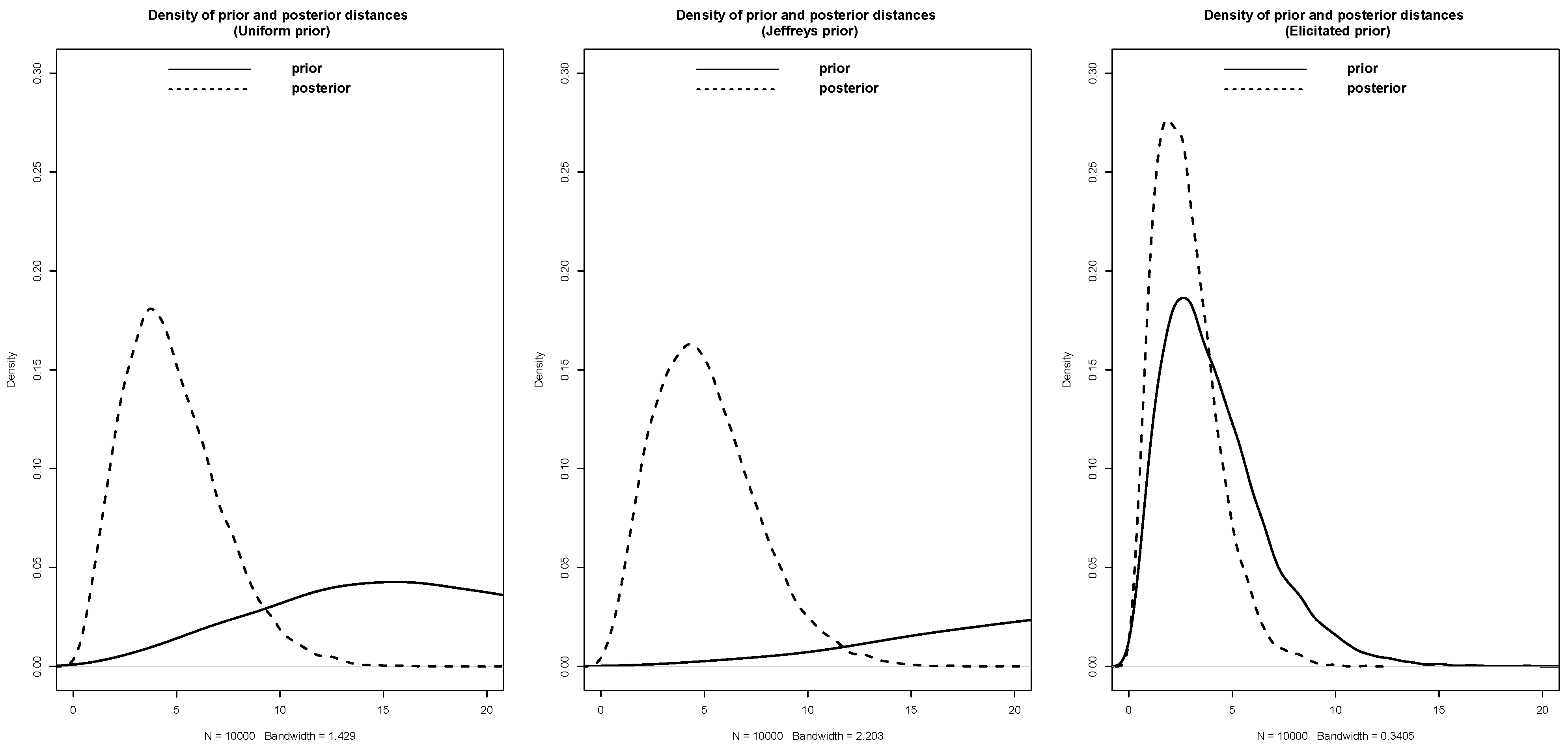
We will use a Bayesian approach to address this problem. We employ three priors: the uniform prior represented by Dirichlet ( 1 , 1 , 1 , 1 , 1 , 1 ) , Jeffreys prior represented by Dirichlet ( 0.5 , 0.5 , 0.5 , 0.5 , 0.5 , 0.5 ) , and the elicited prior Dirichlet (5.83, 5.83, 5.83, 5.83, 5.83, 5.83) obtained using the algorithm proposed by [28], with a lower bound of 0.05 applied to all probabilities. It is worth noting that setting the lower bound in [28] to 0 yields the uniform prior. Additionally, we will include the p-value for the corresponding frequentist test as a reference. The results of our analysis are presented in Table 2. Clearly, both the proposed Bayesian approach, considering the three priors, and the frequentist approach lead to the same conclusion. It should be noted that the uniform prior and the Jefferey prior have a wider spread around zero compared to the elicited prior. As a result, they have higher relative belief ratios in this example. However, this is not practically significant in our case as we calibrate the relative belief ratio through the strength. See Figure 1.
Example 2 
(Operation Trial [5]). In a system consisting of four independent components, let θ j | i denote the probability of successful operation of the ith component, i = 1 , 2 , 3 , 4 . We will test the null hypothesis H 0 2 : θ 1 | 1 = 0.9 , θ 2 | 1 = 0.1 , θ 1 | 2 = 0.9 , θ 2 | 2 = 0.1 , θ 1 | 3 = 0.8 , θ 2 | 3 = 0.2 , θ 1 | 4 = 0.8 , θ 2 | 4 = 0.2 , given that in 50 trials, the components operated as follows (Table 3):
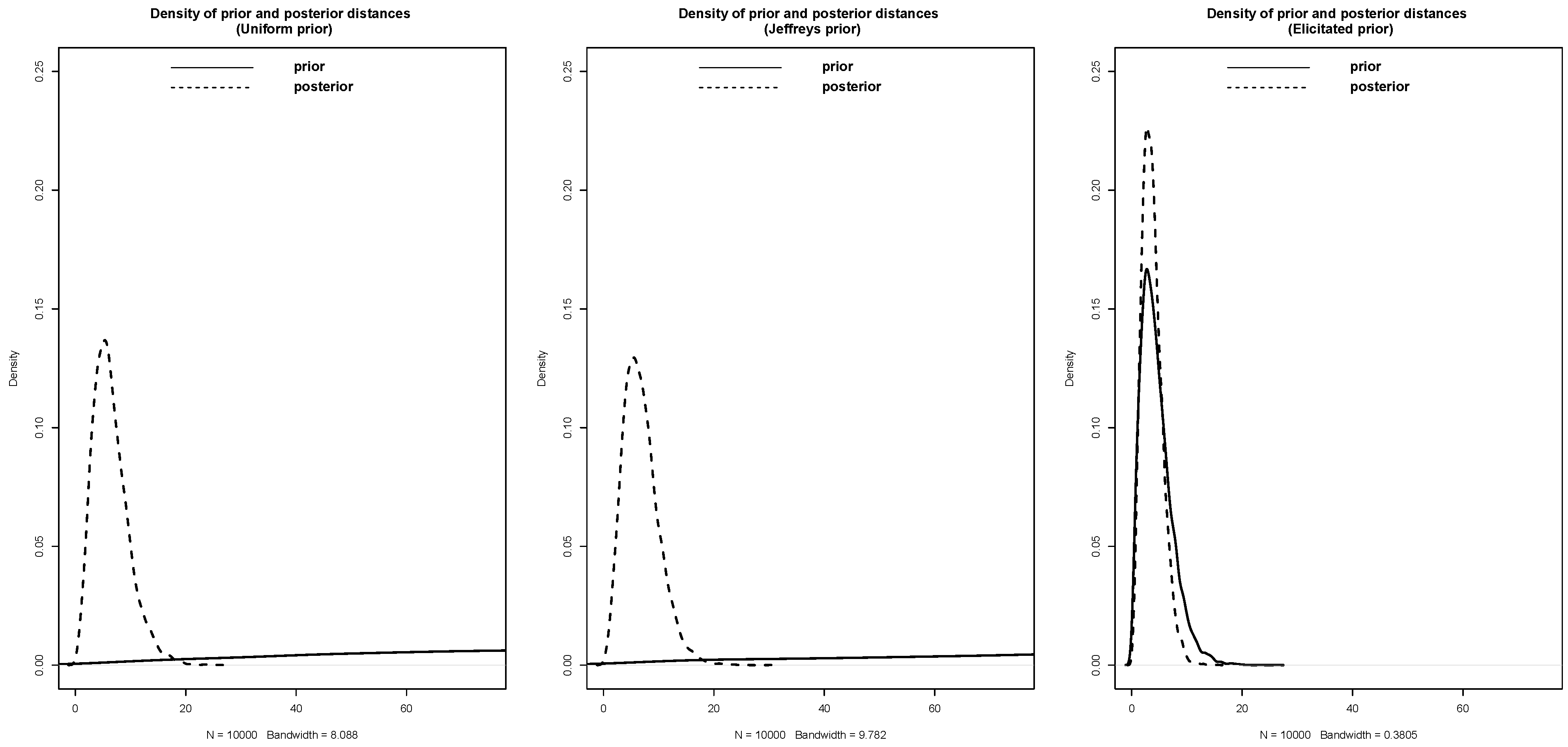
We use the priors: Dirichlet ( 1 , 1 ) , Dirichlet ( 0.5 , 0.5 ) , and Dirichlet ( 33.38 , 5.62 ) . We obtain the latter prior using algorithm of [28], with lower bounds of θ 1 | i = 0.7 and θ 2 | i = 0.1 for all i = 1 , 2 , 3 , 4 . Table 4 displays the results of our analysis. As in Example 1, both the uniform prior and the Jefferey prior exhibit less concentration around zero when compared to the elicited prior. This, in turn, leads to a notably different conclusion than that of the elicited prior and the p-value calculated using the chi-square test. See also Figure 2.
Example 3 
(Clinical Trial; [37]). A study was performed to determine whether the type of cancer differed between blue-collar, white-collar, and unemployed workers. A sample of 100 of each type of worker diagnosed as having cancer was categorized into one of three types of cancer. The results are shown in Table 5. See also Table 12.6 of [37]. The hypothesis to be tested is that the proportions of the three cancer types are the same for all three occupation groups. That is, H 0 3 : θ j | 1 = θ j | 2 = θ j | 3 for all j (types of cancer), where θ j | i is the probability of occupation i having cancer type j.
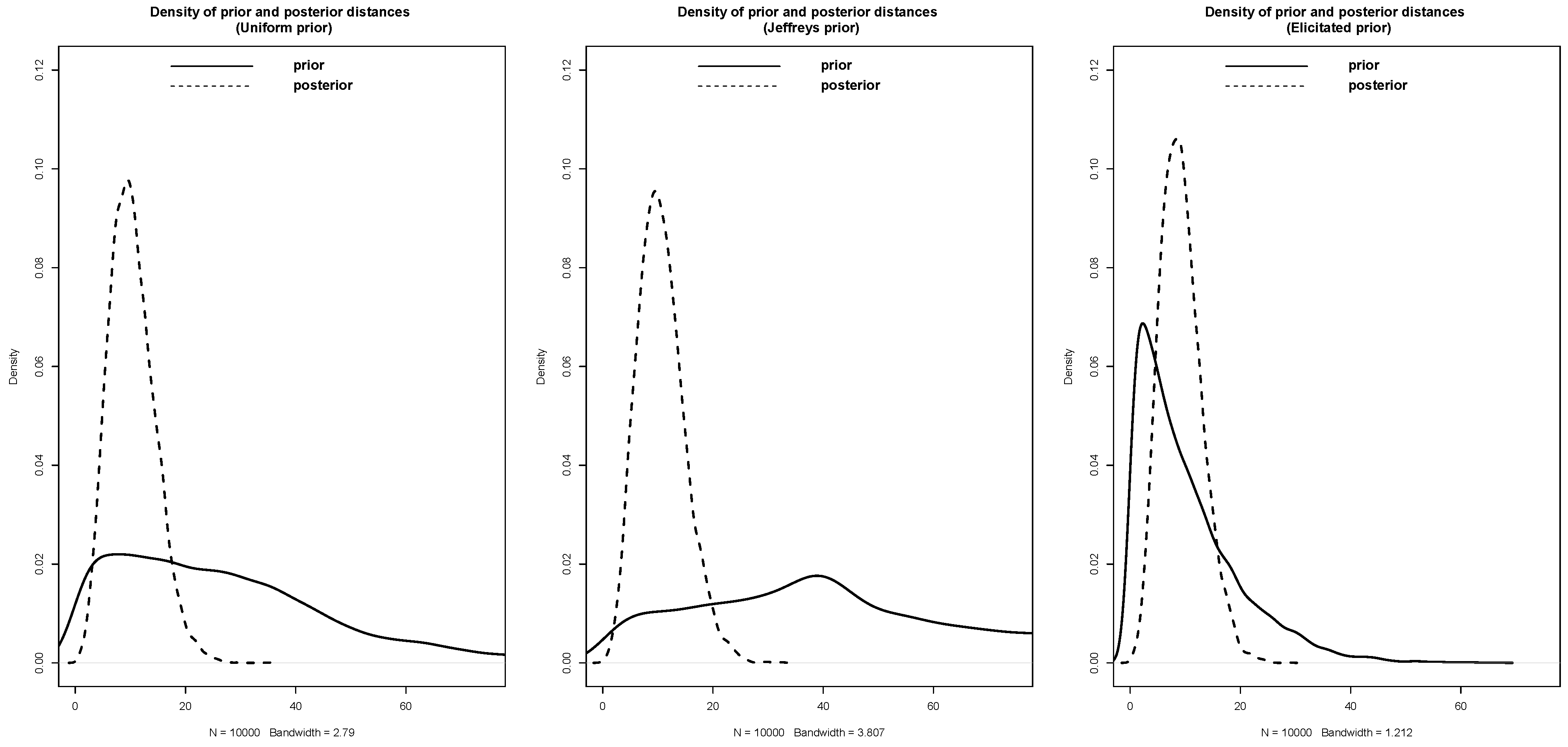
Similar to the previous two examples, we utilize the uniform prior Dirichlet ( 1 , 1 , 1 ) , Jeffreys prior Dirichlet ( 0.5 , 0.5 , 0.5 ) , and the elicited prior Dirichlet ( 3 , 3 , 3 ) . We obtained the elicited prior using the algorithm of [28] by setting a lower bound of 0.05 for all probabilities. Table 6 summarizes the results of our analysis. Similar to the previous examples, Jeffreys prior is not sufficiently concentrated around zero, which makes it inefficient when there is evidence against H 0 . See Figure 3.

5. Concluding Remarks

This study presents a Bayesian method for testing hypotheses related to multinomial distributions. Our approach involves calculating the Kullback–Leibler divergence between two multinomial distributions and comparing the change in distance from the prior to the posterior through the relative belief ratio. To specify the prior distributions, we employ a prior elicitation algorithm. We recommend avoiding the use of Jeffreys prior or the uniform prior unless there is a valid reason to use them. Through several examples, we demonstrated the effectiveness of our approach. Future research may expand our approach to include testing for independence and other related cases.

Author Contributions

Methodology, L.A.-L. and P.C.; Software, P.C., M.D. and K.L.; Resources, K.L.; Writing—review & editing, M.D.; Supervision, L.A.-L. All authors have read and agreed to the published version of the manuscript.

Funding

This research received no external funding.

Data Availability Statement

There are no data associated with this paper.

Acknowledgments

We would like to express our sincere gratitude to the Editor and the anonymous referees for their valuable and constructive comments. Their insightful feedback and suggestions have greatly contributed to the improvement of this paper.

Conflicts of Interest

The authors declare no conflict of interest.

References

  1. Agresti, A. An Introduction to Categorical Data Analysis, 2nd ed.; Wiley: Hoboken, NJ, USA, 2007. [Google Scholar]
  2. Hogg, R.V.; McKean, J.W.; Craig, A.T. Introduction to Mathematical Statistics, 8th ed.; Person: Boston, MA, USA, 2019. [Google Scholar]
  3. Pearson, K. On the criterion that a given system of deviations from the probable in the case of a correlated system of variables is such that it can be reasonably supposed to have arisen from random sampling. Philos. Mag. 1900, 50, 157–175. [Google Scholar] [CrossRef] [Green Version]
  4. Rice, J.A. Mathematical Statistics and Data Analysis, 3rd ed.; Brookes/Cole: Belmont, MA, USA, 2007. [Google Scholar]
  5. Bain, L.J.; Engelhardt, M. Introduction to Probability and Mathematical Statistics; Duxbury Press: North Scituate, MA, USA, 1992. [Google Scholar]
  6. Frey, J. An exact multinomial test for equivalence. Can. J. Stat. 2009, 37, 47–59. [Google Scholar] [CrossRef]
  7. Ostrovski, V. Testing equivalence of multinomial distributions. Stat. Probab. Lett. 2017, 124, 77–82. [Google Scholar] [CrossRef]
  8. Alba-Fernández, M.V.; Jiménez-Gamero, M.D. Equivalence Tests for Multinomial Data Based on ϕ-Divergences. In Trends in Mathematical, Information and Data Sciences. Studies in Systems, Decision and Control; Balakrishnan, N., Gil, M.Á., Martín, N., Morales, D., Pardo, M.d.C., Eds.; Springer: Cham, Switzerland, 2023; Volume 445. [Google Scholar] [CrossRef]
  9. Good, I.J. The population frequencies of species and the estimation of population parameters. Biometrika 1953, 40, 237–264. [Google Scholar] [CrossRef]
  10. Good, I.J. On the estimation of small frequencies in contingency tables. J. R. Stat. Soc. Ser. B 1956, 18, 113–124. [Google Scholar] [CrossRef]
  11. Good, I.J. The Estimation of Probabilities: An Essay on Modern Bayesian Methods; MIT Press: Cambridge, MA, USA, 1965. [Google Scholar]
  12. Good, I.J. A Bayesian significance test for multinomial distributions (with Discussion). J. R. Stat. Soc. Ser. B 1967, 29, 399–431. [Google Scholar]
  13. Lindley, D.V. The Bayesian analysis of contingency tables. Ann. Math. Stat. 1964, 35, 1622–1643. [Google Scholar] [CrossRef]
  14. Altham, P.M.E. Exact Bayesian analysis of a 2 × 2 contingency table, and Fisher’s “exact” significance test. J. R. Stat. Soc. Ser. 1969, 31, 261–269. [Google Scholar] [CrossRef]
  15. Altham, P.M.E. The analysis of matched proportions. Biometrika 1971, 58, 561–576. [Google Scholar] [CrossRef]
  16. Geisser, S. On prior distributions for binary trials. Am. Stat. 1984, 38, 244–247. [Google Scholar]
  17. Bernardo, J.M.; Ramón, J.M. An introduction to Bayesian reference analysis: Inference on the ratio of multinomial parameters. Statistician 1998, 47, 101–135. [Google Scholar] [CrossRef] [Green Version]
  18. Bernardo, J.M.; Smith, A.F.M. Bayesian Theory; Wiley: Hoboken, NJ, USA, 1994. [Google Scholar]
  19. Hashemi, L.; Nandram, B.; Goldberg, R. Bayesian analysis for a single 2×2 table. Stat. Med. 1997, 16, 1311–1328. [Google Scholar] [CrossRef]
  20. Nurminen, M.; Mutanen, P. Exact Bayesian analysis of two proportions. Scand. J. Stat. 1987, 14, 67–77. [Google Scholar]
  21. Agresti, A.; Min, Y. Frequentist performance of Bayesian confidence intervals for comparing proportions in 2×2 contingency tables. Biometrics 2005, 61, 515–523. [Google Scholar] [CrossRef] [PubMed]
  22. Agresti, A.; Hitchcock, D.B. Bayesian inference for categorical data analysis. Stat. Methods Appl. 2005, 14, 297–330. [Google Scholar] [CrossRef]
  23. Leonard, T.; Hsu, J.S.J. The Bayesian Analysis of Categorical Data—A Selective Review. In Aspects of Uncertainty; Freeman, P.R., Smith, A.F.M., Eds.; A Tribute to D. V. Lindley; Wiley: New York, NY, USA, 1994; pp. 283–310. [Google Scholar]
  24. Carota, C. A family of power-divergence diagnostics for goodness-of-fit. Can. J. Stat. 2007, 35, 549–561. [Google Scholar] [CrossRef]
  25. Kim, M.; Nandram, B.; Kim, D.H. Nonparametric Bayesian test of homogeneity using a discretization approach. J. Korean Data Inf. Sci. Soc. 2018, 29, 303–311. [Google Scholar] [CrossRef] [Green Version]
  26. Quintana, F.A. Nonparametric Bayesian analysis for assessing homogeneity in k × l contingency tables with fixed right margin totals. J. Am. Stat. Assoc. 1998, 93, 1140–1149. [Google Scholar] [CrossRef]
  27. Al-Labadi, L.; Cheng, Y.; Fazeli-Asl, F.; Lim, K.; Weng, Y. A Bayesian one-sample test for proportion. Stats 2022, 5, 1242–1253. [Google Scholar] [CrossRef]
  28. Evans, M.; Guttman, I.; Li, P. Prior elicitation, assessment and inference with a Dirichlet prior. Entropy 2017, 19, 564. [Google Scholar] [CrossRef] [Green Version]
  29. Evans, M. Measuring Statistical Evidence Using Relative Belief; Monographs on Statistics and Applied Probability 144; Taylor & Francis Group, CRC Press: Boca Raton, RL, USA, 2015. [Google Scholar]
  30. Abdelrazeq, I.; Al-Labadi, L.; Alzaatreh, A. On one-sample Bayesian tests for the mean. Statistics 2020, 54, 424–440. [Google Scholar] [CrossRef]
  31. Al-Labadi, L. The two-sample problem via relative belief ratio. Comput. Stat. 2021, 36, 1791–1808. [Google Scholar] [CrossRef]
  32. Al-Labadi, L.; Berry, S. Bayesian estimation of extropy and goodness of fit tests. J. Appl. Stat. 2020, 49, 357–370. [Google Scholar] [CrossRef] [PubMed]
  33. Al-Labadi, L.; Evans, M. Optimal robustness results for relative belief inferences and the relationship to prior-data conflict. Bayesian Anal. 2017, 12, 705–728. [Google Scholar] [CrossRef]
  34. Al-Labadi, L.; Evans, M. Prior-based model checking. Can. J. Stat. 2018, 46, 380–398. [Google Scholar] [CrossRef] [Green Version]
  35. Al-Labadi, L.; Patel, V.; Vakiloroayaei, K.; Wan, C. Kullback–Leibler divergence for Bayesian nonparametric model checking. J. Korean Stat. Soc. 2020, 50, 272–289. [Google Scholar] [CrossRef]
  36. Cover, T.M.; Thomas, J.A. Elements of Information Theory, 2nd ed.; Wiley: Hoboken, NJ, USA, 2006. [Google Scholar]
  37. Freund, R.J.; Wilson, W.J.; Mohr, D.L. Statistical Methods, 3rd ed.; Academic Press: Cambridge, MA, USA, 2010. [Google Scholar]
Figure 1. Density plot of distances in Example 1.
Mathematics 11 03007 g001
Figure 2. Density plot of distances in Example 2.
Mathematics 11 03007 g002
Figure 3. Density plot of distances in Example 3.
Mathematics 11 03007 g003
Table 1. Data of Example 1.
123456Total
Observed81151215660
Table 2. The RB and its strength (Str) for Example 1.
PriorRB (Strength)Decision
Uniform15.125 (1)Strong evidence in favor of H 0 1
Jeffreys19.824 (1)Strong evidence in favor of H 0 1
Evan et al.1.900 (1)Strong evidence in favor of H 0 1
p-value0.3027Fail to reject H 0 1 at α = 0.05
Table 3. Data of Example 2.
ComponentSuccessfulFailure
14010
2482
3455
44010
Table 4. The RB and its strength (Str) for Example 2.
PriorRB (Strength)Decision
Uniform20(1)Strong evidence in favor of H 0 2
Jeffreys19.998 (0.000)Weak evidence in favor of H 0 2
Evan et al.0.592 (0.047)Strong evidence against H 0 2
p-value0.030Fail to reject H 0 1 at α = 0.05
Table 5. Data of Example 3.
OccupationType of Cancer
LungStomachOtherTotal
Blue collar531730100
White Collar106723100
Unemployed303040100
Table 6. The RB and its strength (Str) for Example 3.
PriorRB (Strength)Decision
Uniform0.102 (0.010)Strong evidence against H 0
Jeffreys1.874 (0.129)Weak evidence in favor of H 0
Evan et al.0.012 (0.000)Strong evidence against H 0
p-value0.000Reject H 0 1 at α = 0.05
Disclaimer/Publisher’s Note: The statements, opinions and data contained in all publications are solely those of the individual author(s) and contributor(s) and not of MDPI and/or the editor(s). MDPI and/or the editor(s) disclaim responsibility for any injury to people or property resulting from any ideas, methods, instructions or products referred to in the content.