Exploring New Horizons: Advancing Data Analysis in Kidney Patient Infection Rates and UEFA Champions League Scores Using Bivariate Kavya–Manoharan Transformation Family of Distributions

Abstract

In survival analyses, infections at the catheter insertion site among kidney patients using portable dialysis machines pose a significant concern. Understanding the bivariate infection recurrence process is crucial for healthcare professionals to make informed decisions regarding infection management protocols. This knowledge enables the optimization of treatment strategies, reduction in complications associated with infection recurrence and improvement of patient outcomes. By analyzing the bivariate infection recurrence process in kidney patients undergoing portable dialysis, it becomes possible to predict the probability, timing, risk factors and treatment outcomes of infection recurrences. This information aids in identifying the likelihood of future infections, recognizing high-risk patients in need of close monitoring, and guiding the selection of appropriate treatment approaches. Limited bivariate distribution functions pose challenges in jointly modeling inter-correlated time between recurrences with different univariate marginal distributions. To address this, a Copula-based methodology is presented in this study. The methodology introduces the Kavya–Manoharan transformation family as the lifetime model for experimental units. The new bivariate models accurately measure dependence, demonstrate significant properties, and include special sub-models that leverage exponential, Weibull, and Pareto distributions as baseline distributions. Point and interval estimation techniques, such as maximum likelihood and Bayesian methods, where Bayesian estimation outperforms maximum likelihood estimation, are employed, and bootstrap confidence intervals are calculated. Numerical analysis is performed using the Markov chain Monte Carlo method. The proposed methodology’s applicability is demonstrated through the analysis of two real-world data-sets. The first data-set, focusing on infection and recurrence time in kidney patients, indicates that the Farlie–Gumbel–Morgenstern bivariate Kavya–Manoharan–Weibull (FGMBKM-W) distribution is the best bivariate model to fit the kidney infection data-set. The second data-set, specifically that related to UEFA Champions League Scores, reveals that the Clayton Kavya–Manoharan–Weibull (CBKM-W) distribution is the most suitable bivariate model for fitting the UEFA Champions League Scores. This analysis involves examining the time elapsed since the first goal kicks and the home team’s initial goal.

1. Introduction

The analysis of time-to-event data plays a crucial role in understanding the underlying mechanisms and factors that influence outcomes in survival studies. This field encompasses a wide range of applications, including healthcare and sports, where the occurrence of specific events or incidents is of paramount importance.

In healthcare, survival analysis provides valuable insights into the time-to-event outcomes of patients using portable dialysis machines. By examining the recurrence of infections at the catheter insertion site, survival analysis helps identify risk factors, predict the likelihood of future infections, and optimize infection management protocols. This information enables healthcare professionals to make informed decisions, improve treatment strategies, and ultimately enhance patient outcomes.

In sports, survival analysis offers a unique perspective on goal-scoring dynamics and team performance in the Champions League. By analyzing the time elapsed since the first kick goal and the home team’s first goal, survival analysis uncovers patterns and trends in goal-scoring behavior. It provides insights into the probability and timing of goals, the impact of different factors on goal occurrence, and the performance of teams in critical moments of the competition. These insights can aid coaches, analysts, and football enthusiasts in understanding and evaluating team strategies and overall performance in the Champions League.

Under certain exceptional circumstances, it may be necessary to handle two correlated lifetimes T1 and T2, whose individual probabilities are well defined. For example, when studying human organs, such as the kidneys, eyes, ears, or lungs, the intensities of drought, temperatures, floods, earthquakes, and high-wind speeds in two regions, or the results of two teams in the Olympic games, this may be of particular interest. For more information, please refer to Achcar et al. [1] and Bhattacharjee and Misra [2]. Bivariate distributions are important because they can accommodate various types of data that have a parallel clustering system and multiple failures without any order restriction, according to Vincent Raja and Gopalakrishnan [3]. In general, authors often derive bivariate distributions from common baseline distributions, such as Weibull, exponential, gamma, Pareto, and so on, as noted in the literature.

There are various ways of eliciting the bivariate distributions such as the marginal transformation method, Copula method, Marshall and Olkin shock method, conditional specification method, and frailty approach; further details regarding the methods of establishing bivariate distribution can be found in the works of Marshall and Olkin [4], Vincent Raja and Gopalakrishnan [3] and Pathak and Vellaisamy [5].

Copulas have emerged as a significant topic in statistics due to their flexibility and versatility in modeling bivariate and multivariate distributions. One of the primary reasons why copulas are often preferred over other methods is their ability to capture a wide range of dependence patterns between two variables. Unlike some other methods that assume a specific type of dependence structure, copulas can model linear and nonlinear relationships, asymmetric dependence, and tail dependence. Additionally, copulas enable the modeling of the marginal distributions separately from the dependence structure, allowing for more accurate modeling of the data. Furthermore, copulas can be used to model high-dimensional multivariate distributions by linking multiple univariate distributions using a common copula function. These advantages make copulas a valuable tool for researchers and practitioners in many fields, including finance, hydrology, environment, biology, engineering, geophysics, computer science, and medical data analysis.

Statistical models play a crucial role in describing and predicting real-world phenomena. When examining the relationship between two variables, bivariate distributions provide a robust framework. In recent decades, a multitude of bivariate distributions have gained popularity for data modeling across diverse fields. Many authors have extensively utilized the copula function to construct new bivariate models and have applied these statistical models to analyze a wide range of real data-sets. These data-sets span diverse disciplines, including medical research, insurance, sports analysis, psychology and social sciences, economics, climatology and meteorology, environmental studies, and computer science. By harnessing the power of copula functions, these authors have been able to develop sophisticated models that capture the complex dependencies between variables in these domains. Such utilization of copula-based models has significantly enhanced our understanding and predictive capabilities in these fields.

The literature presented in Table 1 highlights several notable studies on bivariate models and their applications to real data. It is important to note that the authors mentioned did not solely focus on constructing a bivariate family with two types of copula and generating three submodels with distinct shapes from each type of copula.

Table 1. Relevant literature.

Model	Type of Copula	Modeling	Authors
The new suggested model (FGMBKM-T family)	FGM copula	Medical data	New
The new suggested model (CBKM-T family)	Clayton copula	Medical data and Sport data	New
Bivariate generalized exponential model	FGM copula	Medical data and simulated data	[1]
Bivariate generalized exponential model	Clayton copula	Sport data	[6]
Bivariate Birnbaum–Saunders model	Gaussian copula	Psychology or Social data	[7]
Bivariate generalized exponential model	Plackett copula	Medical data	[8]
Bivariate modified Weibull model	FGM copula	Medical data	[9]
Bivariate Frechet model	FGM and AMH copula	Economic and Medical data	[10]
Bivariate Weibull model	FGM copula	Medical data	[11]
Bivariate defective Gompertz model	Clayton copula	Medical data	[12]
Bivariate copulas based on the Kumaraswamy distortion	Gumbel, Frank, Clayton, Frank, Galambos copula	Insurance data	[13]
Bivariate generalized Rayleigh model	Clayton copula	Economic data	[14]
Bivariate inverted Topp–Leone model	FGM, Ali–Mikhail–Haq (AMH),	Medical data	[15]
Bivariate XGamma model	FGM copula	Sport data	[16]
Bivariate generalized half-logistic model	FGM copula Plackett, and Clayton copula	Economic data	[17]
Bivariate Nadarajah–Haghighi	FGM copula	Medical data	[18]
Bivariate inverse Lindley model	FGM copula	Climatological or Meteorological data	[19]
Bivariate Power lomax model	FGM copula	Medical data	[20]
Bivariate lomax-G family	FGM copula	Environmental, Medical and Computer science data	[21]

We encounter pioneering contributions, such as the newly suggested Farlie–Gumbel–Morgenstern bivariate Kavya–Manoharan transformation family, denoted as the FGMBKM-T family model, and the Clayton bivariate Kavya–Manoharan transformation family, denoted as the CBKM-T family model. These models utilize the FGM and Clayton copulas and are specifically applied to medical data. Notably, the CBKM-T family model extends its scope to include sports-related data as well. Drawing inspiration from these innovative models, this research aims to explore their effectiveness in capturing the intricate relationships within the respective data-sets. The subsequent rows reveal a rich tapestry of prior studies that have employed copula-based models to investigate various data-sets. These studies span diverse domains, encompassing medical, sport, economic, environmental, psychological, and climatological data. The models in these studies utilize copula types, such as FGM, Clayton, Gaussian, Plackett, and Ali–Mikhail–Haq (AMH), enabling a nuanced understanding of the complex dependence structures present in the data.

It is important to note that the choice of copula type in each model is guided by the unique characteristics of the data-set and the desired properties of the copula function. The selected copulas offer flexibility in capturing and representing different types of interdependence within the data.

By building upon the existing literature and proposing novel models, this research seeks to contribute to the field by uncovering new insights and evaluating the performance of these models across diverse data-sets. The table serves as a valuable resource, providing a foundation for this research and advancing our understanding of copula-based modeling across various contexts.

Sklar [22] derived the probability density function (pdf) and cumulative distribution function (cdf) for the two-dimensional copula function. Consequently, when $Z_1$ and $Z_2$ represent random variables with distribution functions $F_1\left(z_1\right)$ and $F_2\left(z_2\right)$, respectively, the joint cdf and pdf for the bivariate copula can be expressed as follows:

$$F_{Z_1,Z_2}(z_1,z_2)=C(F_1(z_1,{\Delta }_1),F_2(z_2,{\Delta }_2)),$$

(1)

and

$$f_{Z_1,Z_2}(z_1,z_2)=f_1(z_1,{\Delta }_1)f_2(z_2,{\Delta }_2)c(F_1(z_1,{\Delta }_1),F_2(z_2,{\Delta }_2))$$

(2)

Gumbel [23] discussed the Farlie–Gumbel–Morgenstern (FGM) copula, which is one of the most popular parametric families of copulas. The FGM copula and its density are presented as

$$C_{FGM}(u_1,u_2)=u_1{u}_2\left(1+\theta (1-u_1)(1-u_2)\right),-1\le \theta \le 1,$$

(3)

and

$$c_{FGM}(u_1,u_2)=1+\theta (1-2u_1)(1-2u_2),-1\le \theta \le 1,$$

(4)

where $u_1=F_1(z_1,{\Delta }_1)$, $u_2=F_2(z_2,{\Delta }_2)$, and ${\Delta }_1$ and ${\Delta }_2$ are vectors of the parameters for the variables $Z_1$ and $Z_2$, respectively. $\theta$ is a parameter that measures the dependence between the marginals; for further information regarding copulas, please refer to Nelsen [24] and Joe [25]. As a result, the FGM copula is simple and adaptable when handling the construction of bivariate distributions with complex marginal distributions regards to functions.

In addition to the FGM copula, another widely used copula in the literature is the Clayton copula, which was introduced by Clayton [26]. The Clayton copula has a simple expression in terms of its cumulative distribution function (cdf) as

$$C_{Clayton}(u_1,u_2)={\left\{u_1^{-\theta }+u_2^{-\theta }-1\right\}}^{-\frac{1}{\theta }},\theta >0,$$

(5)

where $u_1,u_2\in [0,1]$. Its probability density function (pdf) is given by

$$c_{Clayton}(u_1,u_2)=(1+\theta ){\left(u_1{u}_2\right)}^{-1-\theta }{\left(u_1^{-\theta }+u_2^{-\theta }-1\right)}^{-2-\frac{1}{\theta }},\theta >0.$$

(6)

For more recently information see [27,28,29].

The main objective of this article is to introduce a novel bivariate family of distributions, known as the FGMBKM-T family and CBKM-T family, based on the Kavya–Manoharan transformation family as described by Kavya and Manoharan [30]. These families incorporate two widely used copula functions, namely the Farlie–Gumbel–Morgenstern (FGM) copula and the Clayton copula. We provide several justifications that offer sufficient motivation for exploring the proposed model:

• The new proposed bivariate family exhibits a high degree of flexibility, encompassing various well-known distributions as sub-models.
• By utilizing the bivariate Kavya–Manoharan transformation family based on the FGM copula and Clayton copula, we can generate submodels with distinct shapes. For instance, the FGMBKM-Exponential distribution’s joint hazard rate function (HRF) can exhibit bathtub-shaped, U-shaped, declining, or increasing patterns. Similarly, the CBKM-Exponential distribution can display U-shaped, declining, or increasing HRFs, as well as different tail behaviors. The FGM and Clayton copulas offer flexibility in modeling diverse types of dependence structures, further enhancing the versatility of the bivariate Kavya–Manoharan transformation family.
• Some statistical and mathematical properties of the newly proposed model are investigated.
• Additionally, unexplored mathematical properties of the univariate KM transformation family are examined, which are valuable for analyzing the bivariate KM-T family.
• A maximum likelihood estimation method and Bayesian estimation are employed to estimate the parameters of the FGMBKM-T family and the CBKM-T family.
• Three types of confidence intervals are examined for estimating the unknown parameters: asymptotic intervals, Bayesian credible intervals, and bootstrap intervals.
• The performance of the FGMBKM-T family and CBKM-T family is assessed in comparison to other copula and non-copula distributions.

The main motivation for conducting this research is to utilize the bivariate KM-T family of distributions in various fields, allowing for a comprehensive understanding of the underlying processes and dependencies between variables, which enables healthcare professionals to proactively manage infections and identify high-risk patients, while also providing sports analysts with valuable insights for optimizing team strategies. By incorporating the bivariate KM-T family of distributions, these studies aim to enhance decision making, optimize outcomes, and contribute to the enrichment of healthcare and sports research.

The rest of this paper is structured as follows: the univariate KM-T family and some properties of this family are introduced in Section 2. The FGMBKM-T family is defined in Section 3. The CBKM-T family is introduced in Section 4. In Section 5, measures of dependence for the FGMBKM-T family and the CBKM-T family are discussed. The maximum likelihood estimation and Bayesian estimation procedures are carried out in Section 6. In Section 7, the topic of discussion revolves around confidence intervals. Section 8 demonstrates the adequacy of the new model via a simulation study. In Section 9, the utilization of the kidney patient and football data is discussed. Finally, Section 10 presents a summary of the study and provides essential insights into the FGMBKM-T family and CBKM-T family of distribution.

2. Univariate KM-T Family

In this section, we explore several mathematical properties of the univariate KM transformation family that were not addressed in the original research. These properties are useful for studying the properties of the bivariate KM-T family and include linear representation, quantiles, moments, and weighted moments.

Over the past few years, there has been a growing interest in creating new generators for univariate continuous distributions by adding one or more additional shape parameters to the baseline distribution, see [31,32].

Recently, a new class of distributions that are more parsimonious for estimating lifetime distributions was established. One notable advantage of these transformations is that they do not generalize the distribution, resulting in a simplified distribution in both computation and interpretation. This is due to the fact that they do not introduce any additional parameters beyond those already inherent in the baseline distribution. The advantage of this transformation is that the resulting distribution remains parameter sparse, as no additional parameters are introduced.

Lately, Kavya and Manoharan [30] introduced a new transformation known as the Kavya–Manoharan (KM) transformation family. The cumulative distribution function (cdf) and probability density function (pdf) of the Kavya–Manoharan (KM) transformation family with zero parameter are defined as

$$F(x;\mathsf{\Lambda })=\frac{e}{e-1}\left[1-e^{-G(x;\mathsf{\Lambda })}\right],$$

(7)

and

$$f(x;\mathsf{\Lambda })=\frac{e}{e-1}g(x;\mathsf{\Lambda })e^{-G(x;\mathsf{\Lambda })},$$

(8)

respectively, where $G(x;\mathsf{\Lambda })$ is the baseline distribution, $g(x;\mathsf{\Lambda })=dG(x;\mathsf{\Lambda })/dx$ is the parent pdf in the KM transformation family, and $\mathsf{\Lambda }$ denotes the vector of parameters for baseline cdf G.

This family generates new lifespan models or distributions by utilizing a given baseline distribution, without introducing additional parameters to the model to account for current uncertainty. Instead, the focus is on modeling the lifetime using a process that results in accurate and parsimonious outcomes. The researchers opted for the exponential and Weibull distributions as baseline distributions due to their common usage in survival analyses and reliability theory.

2.1. Linear Representation

We provide a useful linear representation for the MK transformation family pdf in Equation (8). Consider the exponential series

$$e^{-z}=\sum _{k=0}^{\infty }{(-1)}^k\frac{z^k}{k!}.$$

(9)

Applying (9) to $e^{-G(x;\mathsf{\Lambda })}$ and substituting the result in (8) yields

$$f(x;\mathsf{\Lambda })=\sum _{p=0}^{\infty }{a}_p{h}_{p+1}(x;\mathsf{\Lambda }),$$

(10)

where

$$a_p=\frac{e}{e-1}\frac{{(-1)}^p}{(p+1)!},$$

(11)

and $h_{\zeta }=\zeta g\left(x\right)G^{\zeta -1}\left(x\right)$ denotes the exponentiated-G (ExG) class density with power parameter $\zeta >0$. By integrating (10), we obtain

$$F(x;\mathsf{\Lambda })=\sum _{p=0}^{\infty }{a}_p{H}_{p+1}(x;\mathsf{\Lambda }),$$

(12)

where $H_{p+1}$ is the cdf of the ExG family with power parameter $(p+1)$. According to Equation (10), the density of X can be expressed as a linear mixture of exp-G densities. As a result, several mathematical properties of the new family can be derived from the exp-G distribution.

2.2. Quantiles, Ordinary and Incomplete Moments

By inverting (7), the quantile function (qf) of X follows as

$$Q\left(u\right)=F^{-1}\left(u\right)=Q_G\left\{-log\left[1-\frac{(e-1)u}{e}\right]\right\}$$

(13)

where $Q_G\left(u\right)=G^{-1}\left(u\right)$ is the qf of the baseline G distribution and $u\in (0,1)$. A random sample of size n from (7) can be obtained, based on (13), as $X_i=Q_{KM}\left(U_i\right)$, where $U_i\sim$ Uniform$(0,1),i=1,2,\dots ,n$.

Let $Z_{p+1}$ be a R.V, having density $h_{p+1}(x;\mathsf{\Lambda })$. The s-th ordinary moment of X, say ${\mu }_{s,X}^{\prime }$, follows from (10) as

$${\mu }_{s,X}^{\prime }=E\left(X^s\right)=\sum _{p=0}^{\infty }{a}_{p}E\left(Z_{p+1}^s\right),$$

(14)

where

$$E\left(Z_{p+1}^s\right)=(p+1){\int }_{-\infty }^{+\infty }{x}^{s}g(x;\mathsf{\Lambda })G{(x;\mathsf{\Lambda })}^{(p+1)-1}dx,$$

can be numerically evaluated in terms of the baseline qf $Q_G\left(u\right)=G^{-1}\left(u\right)$ as

$$E\left(Z_{p+1}^s\right)=(p+1){\int }_0^1{\left[Q\left(u\right)\right]}^s{u}^{(p+1)-1}du.$$

(15)

Setting s = 1 in (14) yields the mean of X.

The r-th incomplete moment of X is defined by ${\mathsf{\Pi }}_{r,X}\left(z\right)={\int }_{-\infty }^z{x}^{r}f\left(x\right)dx$. We can write from (10)

$${\mathsf{\Pi }}_{r,X}\left(z\right)=\sum _{p=0}^{\infty }{a}_p{\mathsf{\Pi }}_{r,p+1}\left(z\right),$$

(16)

where

$${\mathsf{\Pi }}_{r,P+1}\left(z\right)={\int }_0^{G\left(z\right)}{\left[Q_G\left(u\right)\right]}^r{u}^{(P+1)-1}du.$$

Setting r = 1 in (16) yields the first incomplete moment X. The main applications of ${\mathsf{\Phi }}_1\left(z\right)$ are mean deviations, as well as the Bonferroni and Lorenz curves (see Lorenz [33] and Bonferroni [34]).

2.3. Probability Weighted Moments

The ($s,r$)-th probability weighted moments of X following the KM transformation family are defined by

$${\phi }_{s,r}=E\left(X^s{F}^r\left(X\right)\right)={\int }_{-\infty }^{\infty }{x}^s{F}^r(x;\mathsf{\Lambda })f(x;\mathsf{\Lambda })dx.$$

(17)

Based on Equation (7), we have

$$F^r(x;\mathsf{\Lambda })={\left[\frac{e}{e-1}\right]}^r\sum _{q=0}^r{(-1)}^q\left(\genfrac{}{}{0pt}{}{r}{q}\right)exp\left\{-qG(x;\mathsf{\Lambda })\right\}.$$

(18)

Using (8) and the exponential series, we obtain

$$f(x;\mathsf{\Lambda })F^r(x;\mathsf{\Lambda })={\left[\frac{e}{e-1}\right]}^{r+1}\sum _{q=0}^r\sum _{p=0}^{\infty }\frac{{(-1)}^{q+p}{(q+1)}^p}{p!}\left(\genfrac{}{}{0pt}{}{r}{q}\right)g(x;\mathsf{\Lambda })G^{(p+1)-1}(x;\mathsf{\Lambda }),$$

(19)

or

$$f(x;\mathsf{\Lambda })F^r(x;\mathsf{\Lambda })=\sum _{p=0}^{\infty }{A}_p{h}_{p+1}(x;\mathsf{\Lambda }),$$

(20)

where

$$A_p=\sum _{q=0}^r{\left[\frac{e}{e-1}\right]}^{r+1}\frac{{(-1)}^{q+p}{(q+1)}^p}{p!(p+1)}\left(\genfrac{}{}{0pt}{}{r}{q}\right).$$

Then, we can write

$${\phi }_{s,r}=\sum _{p=0}^{\infty }{A}_p{\int }_{-\infty }^{\infty }{x}^s{h}_{p+1}\left(x\right)dx=\sum _{p=0}^{\infty }{A}_{p}E\left(Z_{P+1}^s\right).$$

(21)

Setting $s=1$ and $r=1$ in (21) gives $\phi =E\left(XF\left(X\right)\right)={\int }_{-\infty }^{\infty }xF(x;\mathsf{\Lambda })f(x;\mathsf{\Lambda })dx.$

3. FGM Bivariate Kavya–Manoharan Transformation (FGMBKM-T) Family

We obtain the cdf and pdf of a random vector $(Z_1,Z_2)$ following the FGMKM-T by applying the Equations (1) and (2) with Equations (7) and (8), and the FGM copula in Equations (3) and (4). They are provided by

$$\begin{array}{ccc}{F}_{FGMBKM-T}(z_1,z_2)={\left[\frac{e}{e-1}\right]}^2\left[1-e^{-G(z_1;{\mathsf{\Lambda }}_1)}\right]\left[1-e^{-G(z_2;{\mathsf{\Lambda }}_2)}\right]\hfill & \hfill & \\ \hspace{1em}\hspace{1em}\hspace{1em}\hspace{1em}\left\{1+\theta \left[1-\frac{e}{e-1}\left(1-e^{-G(z_1;{\mathsf{\Lambda }}_1)}\right)\right]\left[1-\frac{e}{e-1}\left(1-e^{-G(z_2;{\mathsf{\Lambda }}_2)}\right)\right]\right\},-1\le \theta \le 1,\hfill \end{array}$$

(22)

$$\begin{array}{ccc}{f}_{FGMBKM-T}(z_1,z_2)={\left[\frac{e}{e-1}\right]}^{2}g(z_1;{\mathsf{\Lambda }}_1)g(z_2;{\mathsf{\Lambda }}_2)e^{-G(z_1;{\mathsf{\Lambda }}_1)-G(z_2,{\mathsf{\Lambda }}_2)}\hfill & \hfill & \\ \hspace{1em}\hspace{1em}\hspace{1em}\hspace{1em}\left\{1+\theta \left[1-\frac{2e}{e-1}\left(1-e^{-G(z_1;{\mathsf{\Lambda }}_1)}\right)\right]\left[1-\frac{2e}{e-1}\left(1-e^{-G(z_2;{\mathsf{\Lambda }}_2)}\right)\right]\right\},-1\le \theta \le 1,\hfill \end{array}$$

(23)

respectively, with the restrictions of the variables and parameters already stated.

3.1. Reliability and Hazard Rate Function of FGMBKM-T Family

In the reliability analysis, it is often appropriate to express a joint survival (or reliability) function (sf or rf), denoted as $R_{Z_1,Z_2}(z_1,z_2)$, as a copula of its marginal survival functions, namely, $R_{Z_1}\left(z_1\right)$ and $R_{Z_2}\left(z_2\right)$. This concept was introduced by Osmetti [35]. Therefore, the joint survival function for the copula can be expressed as

$$R_{Z_1,Z_2}(z_1,z_2)=C(R_{Z_1}\left(z_1\right),R_{Z_2}\left(z_2\right)).$$

(24)

The expression for the joint survival function, based on the FGM copula, is as follows:

$$R_{FGM}(z_1,z_2)=R_{Z_1}\left(z_1\right)R_{Z_2}\left(z_2\right)\left[1+\theta \left(1-R_{Z_1}\left(z_1\right)\right)\left(1-R_{Z_2}\left(z_2\right)\right)\right],-1\le \theta \le 1.$$

Hence, the reliability function of the FGMBKM-T family can be expressed as

$$\begin{array}{cc}\hfill R_{FGMBKM-T}(z_1,z_2)=& \left[1-\frac{e}{e-1}\left(1-e^{-G(z_1;{\mathsf{\Lambda }}_1)}\right)\right]\left[1-\frac{e}{e-1}\left(1-e^{-G(z_2;{\mathsf{\Lambda }}_2)}\right)\right]\hfill \\ \hfill & \left[1+\theta \frac{e^2}{{(e-1)}^2}\left(1-e^{-G(z_1;{\mathsf{\Lambda }}_1)}\right)\left(1-e^{-G(z_2;{\mathsf{\Lambda }}_2)}\right)\right],-1\le \theta \le 1.\hfill \end{array}$$

(25)

According to Basu [36], the bivariate hazard rate function is

$$h_{Z_1,Z_2}(z_1,z_2)=\frac{f_{Z_1,Z_2}(z_1,z_2)}{R_{Z_1,Z_2}(z_1,z_2)}.$$

(26)

The hazard rate function of FGMBKM-T family is indicated as

$$\begin{array}{ccc}{h}_{FGMBKM-T}(z_1,z_2)=\frac{g(z_1;{\mathsf{\Lambda }}_1)e^{-G(z_1;{\mathsf{\Lambda }}_1)}}{1-\frac{e}{e-1}\left(1-e^{-G(z_1;{\mathsf{\Lambda }}_1)}\right)}\frac{e^{2}g(z_2;{\mathsf{\Lambda }}_2)e^{-G(z_2;{\mathsf{\Lambda }}_2)}}{{(e-1)}^2\left[1-\frac{e}{e-1}\left(1-e^{-G(z_2;{\mathsf{\Lambda }}_2)}\right)\right]}\hfill & \hfill & \\ \hspace{1em}\hspace{1em}\hspace{1em}\hspace{1em}\frac{\left\{1+\theta \left[1-\frac{2e}{e-1}\left(1-e^{-G(z_1;{\mathsf{\Lambda }}_1)}\right)\right]\left[1-\frac{2e}{e-1}\left(1-e^{-G(z_2;{\mathsf{\Lambda }}_2)}\right)\right]\right\}}{\left\{1+\theta \frac{e^2}{{(e-1)}^2}\left(1-e^{-G(z_1;{\mathsf{\Lambda }}_1)}\right)\left(1-e^{-G(z_2;{\mathsf{\Lambda }}_2)}\right)\right\}},-1\le \theta \le 1.\hfill \end{array}$$

(27)

3.2. Special FGMBKM-T Family of Distributions

We presented three special models of the FGMBKM-T family of distributions in this section. When both the cdf $G\left(z\right)$ and pdf $g\left(z\right)$ have straightforward analytic expressions, the pdf (23) is most practical. Taking the baseline distributions, we focus on three sub-models of this transformation: including exponential (Ex), Weibull (W) and Pareto (Pa). The cdf and pdf of the baseline models are displayed in Table 2. The FGMBKM-T is a very adaptable model in the sub-models of the FGMBKM transformation that approaches various bivariate distributions as its parameters are altered.

Table 2. Baseline models in cdf and pdf.

Model	cdf:    $\mathit{G}(\mathit{z};\mathbf{\Lambda })$	Pdf:    $\mathit{g}(\mathit{z};\mathbf{\Lambda })$
Exponential	$1-e^{-\left(bz\right)}$             ; z > 0	$b{e}^{-\left(bz\right)}$
Weibull	$1-exp\left[-{\left(bz\right)}^a\right]$ ; z > 0	$a{b}^a{z}^{a-1}exp\left[-{\left(bz\right)}^a\right]$
Pareto	$1-{(1+z)}^{-v}$      ; z > 0	$v{(1+z)}^{-(1+v)}$

3.2.1. FGMBKM-Exponential (FGMBKM-Ex) Distribution

By using KM-T family and exponential distribution to obtain KM-Exponential (KM-Ex) distribution, the cdf, pdf and sf of FGMBKM-Ex distribution (for $z_j>0$ and $b_j>0$ for $j=1,2$) are

$$\begin{array}{cc}\hfill F_{FGMBKM-Ex}(z_1,z_2)=& {\left[\frac{e}{e-1}\right]}^2{\varpi }_1(z_1,b_1){\varpi }_2(z_2,b_2)\hfill \\ \hfill & \left\{1+\theta \left(1-\frac{e}{e-1}{\varpi }_1(z_1,b_1)\right)\left(1-\frac{e}{e-1}{\varpi }_2(z_2,b_2)\right)\right\},\hfill \end{array}$$

(28)

$$\begin{array}{cc}\hfill f_{FGMBKM-Ex}(z_1,z_2)=& \frac{b_1{e}^{-b_1{z}_1}{e}^{e^{-b_1{z}_1}}}{e-1}\frac{b_2{e}^{-b_2{z}_2}{e}^{e^{-b_2{z}_2}}}{e-1}\hfill \\ \hfill & \left\{1+\theta \left(1-\frac{2e}{e-1}{\varpi }_1(z_1,b_1)\right)\left(1-\frac{2e}{e-1}{\varpi }_2(z_2,b_2)\right)\right\},\hfill \end{array}$$

(29)

and

$$\begin{array}{cc}\hfill R_{FGMBKM-Ex}(z_1,z_2)=& \left[1-\frac{e}{e-1}{\varpi }_1(z_1,b_1)\right]\left[1-\frac{e}{e-1}{\varpi }_2(z_2,b_2)\right]\hfill \\ \hfill & \left[1+\theta \frac{e^2}{{(e-1)}^2}{\varpi }_1(z_1,b_1){\varpi }_2(z_2,b_2)\right].\hfill \end{array}$$

(30)

where ${\varpi }_j(x_j,b_j)=\left(1-e^{-\left(1-e^{-b_j{x}_j}\right)}\right)$. The hazard rate function of FGMBKM-EX distribution is given as

$$\begin{array}{cccc}\hfill h_{FGMBKM-Ex}(z_1,z_2)=& \frac{1}{{[e-1]}^2}\frac{b_1{e}^{-b_1{z}_1}{e}^{e^{-b_1{z}_1}}}{\left[1-\frac{e}{e-1}{\varpi }_1(z_1,b_1)\right]}\frac{b_2{e}^{-b_2{z}_2}{e}^{e^{-b_2{z}_2}}}{\left[1-\frac{e}{e-1}{\varpi }_2(z_2,b_2)\right]}\hfill & \hfill & \\ \hfill & \frac{\left\{1+\theta \left[1-\frac{2e}{e-1}{\varpi }_1(z_1,b_1)\right]\left[1-\frac{2e}{e-1}{\varpi }_2(z_2,b_2)\right]\right\}}{\left\{1+\theta \frac{e^2}{{(e-1)}^2}{\varpi }_1(z_1,b_1){\varpi }_2(z_2,b_2)\right\}}.\hfill \end{array}$$

(31)

A graphical illustration of the joint pdf and joint hazard rate of the FGMBKM-Ex model using various parameter combinations is shown in Figure 1. The joint pdf and joint hazard of the FGMBKM-Ex model are decreasing, decreasing, and J-shaped, respectively, depending on the values of the parameter. The joint hazard of the FGMBKM-Ex model can also be bathtub-shaped, U-shaped, declining, or increasing.

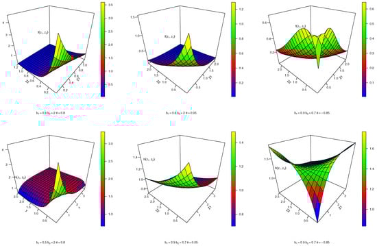
Figure 1. Joint pdf and joint hazard rate of FGMBKM-Ex distribution.

3.2.2. FGMBKM-Weibull (FGMBKM-W) Distribution

By using the KM-T family and Weibull distribution to obtain the KM-Weibull (KM-W) distribution, the cdf and pdf of the FGMBKM-W distribution (for $z_j>0,b_j>0$ and $a_j>0$) are

$$\begin{array}{cc}\hfill F_{FGMBKM-W}(z_1,z_2)=& {\left[\frac{e}{e-1}\right]}^2{\varpi }_1(z_1,b_1,a_1){\varpi }_2(z_2,b_2,a_2)\hfill \\ \hfill & \left\{1+\theta \left(1-\frac{e}{e-1}{\varpi }_1(z_1,b_1,a_1)\right)\left(1-\frac{e}{e-1}{\varpi }_2(z_2,b_2,a_2)\right)\right\},\hfill \end{array}$$

(32)

$$\begin{array}{cc}\hfill f_{FGMBKM-W}(z_1,z_2)=& \frac{a_1{b}_1^{a_1}}{e-1}{z}_1^{a_1-1}{e}^{-{\left(b_1{z}_1\right)}^{a_1}}{e}^{e^{-{\left(b_1{z}_1\right)}_1^a}}\frac{a_2{b}_2^{a_2}}{e-1}{z}_2^{a_2-1}{e}^{-{\left(b_2{z}_2\right)}^{a_2}}{e}^{e^{-{\left(b_2{z}_2\right)}^{a_2}}}\hfill \\ \hfill & \left\{1+\theta \left(1-\frac{2e}{e-1}{\varpi }_1(z_1,b_1,a_1)\right)\left(1-\frac{2e}{e-1}{\varpi }_2(z_2,b_2,a_2)\right)\right\},\hfill \end{array}$$

(33)

where ${\varpi }_j(x_j,b_j,a_j)=\left(1-e^{-\left(1-e^{-{\left(b_j{x}_j\right)}^{a_j}}\right)}\right)$.

3.2.3. FGMBKM-Pareto (FGMBKM-Pa) Distribution

By using the KM-T family and Pareto distribution to obtain the KM-Pareto (KM-Pa) distribution, the cdf and pdf of the FGMBKM transformation (for $z_j>0$ and $v_j>0$) are

$$\begin{array}{c}{F}_{FGMBKM-Pa}(z_1,z_2)={\left[\frac{e}{e-1}\right]}^2{\varpi }_1(z_1,v_1){\varpi }_2(z_2,v_2)\hfill \\ \hspace{1em}\hspace{1em}\hspace{1em}\hspace{1em}\left\{1+\theta \left(1-\frac{e}{e-1}{\varpi }_1(z_1,v_1)\right)\left[(1-\frac{e}{e-1}{\varpi }_2(z_2,v_2)\right)\right\},\hfill \end{array}$$

(34)

$$\begin{array}{cc}\hfill f_{FGMBKM-Pa}(z_1,z_2)=& \frac{v_1}{e-1}{(1+z_1)}^{-(1+v_1)}{e}^{{(1+z_1)}^{-v_1}}\frac{v_2}{e-1}{(1+z_2)}^{-(1+v_2)}{e}^{{(1+z_2)}^{-v_2}}\hfill \\ \hfill & \left\{1+\theta \left(1-\frac{2e}{e-1}{\varpi }_1(z_1,v_1)\right)\left(1-\frac{2e}{e-1}{\varpi }_2(z_2,v_2)\right)\right\},\hfill \end{array}$$

(35)

where ${\varpi }_j(x_j,v_j)=\left(1-e^{{(1+x_j)}^{-v_j}-1}\right)$.

3.3. Statistical Properties of the FGMBKM-T Family

In this section, we discuss some statistical properties of the FGMBKM-T family as presented by Equations (22) and (23). The marginal distributions, product moments, moment generating function, conditional distribution and generating random variables are derived.

3.3.1. The Marginal Distributions

The marginals distributions of the joint FGMBKM-T family’s pdf stated in Equation (23) for $z_1$ and $z_2$, respectively, are KM-transformation marginals and are given as

$$f_{Z_1,FGM}(z_1,{\mathsf{\Lambda }}_1)=\frac{e}{e-1}g(z_1;{\mathsf{\Lambda }}_1)e^{-G(z_1;{\mathsf{\Lambda }}_1)},$$

(36)

and

$$f_{Z_2,FGM}(z_2,{\mathsf{\Lambda }}_2)=\frac{e}{e-1}g(z_2;{\mathsf{\Lambda }}_2)e^{-G(z_2;{\mathsf{\Lambda }}_2)},$$

(37)

which are the KM-T family as given in Equations (36) and (37).

3.3.2. Conditional Distribution

For $l\ne j$ with $l,j=1,2$, we have the following:

(i)

The conditional probability distribution of $Z_l$ given $Z_j=z_j$ is

$$\begin{array}{cccc}\hfill f_{Z_l\mid Z_j,FGM}(z_l\mid z_j)=& \frac{f_{Z_l,Z_j}(z_l,z_j)}{f_{Z_j}\left(z_j\right)}\hfill & \hfill & \\ \hfill & =\frac{e}{e-1}g(z_l;{\mathsf{\Lambda }}_l)e^{-G(z_l;{\mathsf{\Lambda }}_l)}\hfill & \hfill & \\ \hfill & \left\{1+\theta \left[1-2F_l(z_l,{\mathsf{\Lambda }}_l)\right]\left[1-2F_j(z_j,{\mathsf{\Lambda }}_j)\right]\right\},-1\le \theta \le 1,\hfill \end{array}$$

(38)

where $F_l(z_l,{\mathsf{\Lambda }}_l)=\frac{e}{e-1}\left(1-e^{-G(z_l;{\mathsf{\Lambda }}_l)}\right)$ and $F_j(z_j,{\mathsf{\Lambda }}_j)=\frac{e}{e-1}\left(1-e^{-G(z_j;{\mathsf{\Lambda }}_j)}\right)$.

(ii)

The conditional cdf of $Z_l$ given $Z_j=z_j$ is

$$\begin{array}{cc}\hfill F_{Z_l\mid Z_j,FGM}(z_l\mid z_j)& =P(Z_l\le z_l\mid Z_j=z_j)\hfill \\ \hfill & =F_l(z_l,{\mathsf{\Lambda }}_l)\left\{1+\theta \left[1-F_l(z_l,{\mathsf{\Lambda }}_l)\right]\left[1-2F_j(z_j,{\mathsf{\Lambda }}_j)\right]\right\},-1\le \theta \le 1.\hfill \end{array}$$

(39)

(iii)

The conditional survival of $Z_l$ given $Z_j=z_j$ is

$$\begin{array}{cc}\hfill R_{Z_l\mid Z_j,FGM}(z_l\mid z_j)& =P(Z_l>z_l\mid Z_j=z_j)\hfill \\ \hfill & =\left[1-F_l(z_l,{\mathsf{\Lambda }}_l)\right]\left\{1-\theta F_l(z_l,{\mathsf{\Lambda }}_l)\left[1-2F_j(z_j,{\mathsf{\Lambda }}_j)\right]\right\},-1\le \theta \le 1.\hfill \end{array}$$

(40)

(iv)

The conditional expectation of $Z_l$ given $Z_j=z_j$ in the FGMBKM-T family using the conditional density of $Z_l$ given $Z_j=z_j$ in (38) is

$$E(z_l\mid z_j)={\mu }_{z_l}^{\prime }\left[1+\theta -2\theta F_j(z_j,{\mathsf{\Lambda }}_j)+{\phi }_{z_l}\left(4\theta F_j(z_j,{\mathsf{\Lambda }}_j)-2\theta \right)\right],-1\le \theta \le 1,$$

(41)

where ${\mu }_{z_l}^{\prime }$ and ${\phi }_{z_l}$ are defined by Equations (14) and (21) by setting $s=r=1$, respectively.

3.3.3. Generating Random Variables

A bivariate sample of the FGMBKM-T family based on the conditional method (39) can be generated as follows:

(1)

Generate V and U independently from a uniform$(0,1)$ distribution.

(2)

Set $z_1=Q_{BFGBMK-T}=G^{-1}\left\{-log\left[1-\frac{(e-1)U}{e}\right]\right\}$.

(3)

$F_{Z_2\mid Z_1,FGM}(z_2\mid z_1)=U$ in (39) to obtain $z_2$ using numerical analysis, such as Newton–Raphson, etc.

(4)

Repeat 1–3 (n) times to obtain $(z_{1i},z_{2i})$, $i=1,2,\dots ,n$.

3.3.4. Moment Generating Function

The moment generating function of $(Z_1,Z_2)$ following the FGMBKM-T family is obtained as

$$\begin{array}{cc}\hfill M_{Z_1,Z_2}(t_1,t_2)=& E\left(e^{t_1{Z}_1}{e}^{t_2{Z}_2}\right)=\sum _{n_1=0}^{\infty }\sum _{n_2=0}^{\infty }\frac{{\left(t_1\right)}^{n_1}}{n_1!}\frac{{\left(t_2\right)}^{n_2}}{n_2!}{\mu }_{n_1,z_1}^{\prime }{\mu }_{n_2,z_2}^{\prime }\hfill \\ \hfill & \left[1+\theta -2\theta {\mathsf{\Psi }}_{n_1}-2\theta {\mathsf{\Psi }}_{n_2}+4\theta {\mathsf{\Psi }}_{n_1}{\mathsf{\Psi }}_{n_2}\right],-1\le \theta \le 1.\hfill \end{array}$$

(42)

where ${\mu }_{n_j,Z_j}^{\prime }$ and ${\phi }_{n_j,1}$ are defined in Equations (14) and (21), and ${\mathsf{\Psi }}_j=\frac{{\phi }_{n_j,1}}{{\mu }_{n_j,Z_j}^{\prime }}$ for $j=1,2$.

3.3.5. Product Moments

For any positive real numbers $s_1$ and $s_2$, we can calculate the product moments about the origin of ($Z_1,Z_2$) following the FGMBKM-T family as

$${\mu }_{s_1{s}_2}^{\prime }=E\left(Z_1^{s_1}{Z}_2^{s_2}\right)={\mu }_{s_1}^{\prime }{\mu }_{s_2}^{\prime }\left[1+\theta -2\theta {\mathsf{\Omega }}_{s_2}-2\theta {\mathsf{\Omega }}_{s_1}+4\theta {\mathsf{\Omega }}_{s_1}{\mathsf{\Omega }}_{s_2}\right],-1\le \theta \le 1,$$

(43)

where ${\mu }_{s_j,z_j}^{\prime }$ and ${\phi }_{s_j,1}$ are defined in Equations (14) and (21), and ${\mathsf{\Omega }}_j=\frac{{\phi }_{s_j,1}}{{\mu }_{s_j,z_j}^{\prime }}$ for $j=1,2$. Various measures of moment skewness and kurtosis can be introduced by using the product moments. From (43), the covariance and correlation ($\rho$) between $Z_1$ and $Z_2$ are calculated as follows:

$$cov(Z_1,Z_2)={\mu }_{z_1}^{\prime }{\mu }_{z_2}^{\prime }\theta \left[1-2{\mathsf{\Omega }}_{z_2}-2{\mathsf{\Omega }}_{z_1}+4{\mathsf{\Omega }}_{z_1}{\mathsf{\Omega }}_{z_2}\right],-1\le \theta \le 1,$$

(44)

and

$$\rho (Z_1,Z_2)=\frac{\theta \left[1-2{\mathsf{\Omega }}_{z_2}-2{\mathsf{\Omega }}_{z_1}+4{\mathsf{\Omega }}_{z_1}{\mathsf{\Omega }}_{z_2}\right]}{\sqrt{\frac{{\mu }_{2_{z_1}}^{\prime }}{{{\mu }_{z_1}^{\prime }}^2}-1}\sqrt{\frac{{\mu }_{2_{z_2}}^{\prime }}{{{\mu }_{z_2}^{\prime }}^2}-1}},-1\le \theta \le 1,$$

(45)

where ${\mu }_{2_{z_1}}^{\prime }={\int }_{-\infty }^{\infty }{z_1}^{2}g(z_1;{\mathsf{\Lambda }}_1)d{z}_1$ and ${\mu }_{2_{z_2}}^{\prime }={\int }_{-\infty }^{\infty }{z_2}^{2}g(z_2;{\mathsf{\Lambda }}_2)d{z}_2$ We notice that $\rho =0$ when $\theta =0$, implying that $Z_1$ and $Z_2$ are independent.

4. Clayton Bivariate Kavya–Manoharan Transformation (CBKM-T) Family

We derive the cdf and pdf of a random vector $(Z_1,Z_2)$ using the Clayton BKM-T by using Equations (1) and (2) in conjunction with Equations (7) and (8), and incorporating the Clayton copula from Equations (5) and (6), which are provided as follows:

$$\begin{array}{cc}\hfill F_{CBKM-T}(z_1,z_2)=& {\left\{{\left[\frac{e}{e-1}\left(1-e^{-G(z_1;\mathsf{\Lambda })}\right)\right]}^{-\theta }+{\left[\frac{e}{e-1}\left(1-e^{-G(z_2;\mathsf{\Lambda })}\right)\right]}^{-\theta }-1\right\}}^{-\frac{1}{\theta }},\theta >0;\hfill \end{array}$$

(46)

$$\begin{array}{cccc}\hfill f_{CBKM-T}(z_1,z_2)=& {\left[\frac{e}{e-1}\right]}^{-2\theta }g(z_1;{\mathsf{\Lambda }}_1)g(z_2;{\mathsf{\Lambda }}_2)e^{-G(z_1;{\mathsf{\Lambda }}_1)-G(z_2,{\mathsf{\Lambda }}_2)}(1+\theta )\hfill & \hfill & \\ \hfill & {\left\{\left(1-e^{-G(z_1;{\mathsf{\Lambda }}_1)}\right)\left(1-e^{-G(z_2;{\mathsf{\Lambda }}_2)}\right)\right\}}^{-1-\theta }\theta >0;\hfill & \hfill & \\ \hfill & {\left\{{\left[\frac{e}{e-1}\left(1-e^{-G(z_1;{\mathsf{\Lambda }}_1)}\right)\right]}^{-\theta }+{\left[\frac{e}{e-1}\left(1-e^{-G(z_2;{\mathsf{\Lambda }}_2)}\right)\right]}^{-\theta }-1\right\}}^{-2-\frac{1}{\theta }},\hfill \end{array}$$

(47)

respectively, with the limitations of the variables and parameters already mentioned.

4.1. Reliability and Hazard Rate Function of CBKM-T Family

The reliability of CBKM-T family can be obtained according to the Clayton copula and Equation (24) as

$$R_{Clayton}(z_1,z_2)={\left\{R_{Z_1}{\left(z_1\right)}^{-\theta }+R_{Z_2}{\left(z_2\right)}^{-\theta }-1\right\}}^{-\frac{1}{\theta }},\theta >0.$$

(48)

The joint survival function for the CBKM-T family can be expressed as follows:

$$\begin{array}{c}\hfill R_{CBKM-T}(z_1,z_2)={\left\{{\left[1-F_1(z_1,{\mathsf{\Lambda }}_1)\right]}^{-\theta }+{\left[1-F_2(z_2,{\mathsf{\Lambda }}_2)\right]}^{-\theta }-1\right\}}^{-\frac{1}{\theta }},\theta >0,\end{array}$$

(49)

where $F_1(z_1,{\mathsf{\Lambda }}_1)=\frac{e}{e-1}\left(1-e^{-G(z_1;{\mathsf{\Lambda }}_1)}\right)$ and $F_2(z_2,{\mathsf{\Lambda }}_2)=\frac{e}{e-1}\left(1-e^{-G(z_2;{\mathsf{\Lambda }}_2)}\right)$.

The hazard rate function of CBKM-T family is indicated as

$$\begin{array}{cccc}\hfill h_{BCBKM-T}(z_1,z_2)& ={\left[\frac{e}{e-1}\right]}^{-2\theta }g(z_1;{\mathsf{\Lambda }}_1)g(z_2;{\mathsf{\Lambda }}_2)e^{-G(z_1;{\mathsf{\Lambda }}_1)-G(z_2,{\mathsf{\Lambda }}_2)}(1+\theta )\hfill & \hfill & \\ \hfill & {\left\{\left(1-e^{-G(z_1;{\mathsf{\Lambda }}_1)}\right)\left(1-e^{-G(z_2;{\mathsf{\Lambda }}_2)}\right)\right\}}^{-1-\theta }\hfill & \hfill & \\ \hfill & \frac{{\left\{{\left[\frac{e}{e-1}\left(1-e^{-G(z_1;{\mathsf{\Lambda }}_1)}\right)\right]}^{-\theta }+{\left[\frac{e}{e-1}\left(1-e^{-G(z_2;{\mathsf{\Lambda }}_2)}\right)\right]}^{-\theta }-1\right\}}^{-2-\frac{1}{\theta }}}{{\left\{{\left[1-\frac{e}{e-1}\left(1-e^{-G(z_1;{\mathsf{\Lambda }}_1)}\right)\right]}^{-\theta }+{\left[1-\frac{e}{e-1}\left(1-e^{-G(z_2;{\mathsf{\Lambda }}_2)}\right)\right]}^{-\theta }-1\right\}}^{-\frac{1}{\theta }}}.\hfill \end{array}$$

(50)

4.2. Special CBKM-T Distributions

In this section, we introduce three special models of the CBKM-T family of distributions. The most practical probability density function (pdf) for this family is given by Equation (47), which is particularly useful when the cumulative distribution function (cdf) $G\left(z\right)$ and pdf $g\left(z\right)$ can be expressed analytically. We focus on the Clayton copula with three baseline distributions: exponential (Ex), Weibull (W), and Pareto (Pa), and their cdf and pdf are listed in Table 2.

The sub-models of the CBKM-T family are highly adaptable, and the CBKM-T models, in particular, are capable of approaching various bivariate distributions by adjusting their parameters.

4.2.1. CBKM-Exponential (CBKM-Ex) Distribution

Obtaining the KM-Exponential (KM-Ex) distribution involves using the KM-T family and exponential distribution. This allows us to obtain the cdf, pdf, and sf of the CBKM-Ex distribution (for $z_j>0$ and $b_j>0$ for $j=1,2$) as follows:

$$\begin{array}{cc}\hfill F_{CBKM-Ex}(z_1,z_2)=& {\left\{{\left[\frac{e}{e-1}{\varpi }_1(z_1,b_1)\right]}^{-\theta }+{\left[\frac{e}{e-1}{\varpi }_2(z_2,b_2)\right]}^{-\theta }-1\right\}}^{-\frac{1}{\theta }},\hfill \end{array}$$

(51)

$$\begin{array}{cc}\hfill f_{CBKM-Ex}(z_1,z_2)=& {\left[\frac{e}{e-1}\right]}^{-2\theta }{b}_1{e}^{-\left(b_1{z}_1\right)}{b}_2{e}^{-\left(b_2{z}_2\right)}{e}^{e^{-\left(b_1{z}_1\right)}+e^{-\left(b_2{z}_2\right)}-2}\hfill \\ \hfill & (1+\theta ){\left\{{\varpi }_1(z_1,b_1){\varpi }_2(z_2,b_2)\right\}}^{-1-\theta }\hfill \\ \hfill & {\left\{{\left[\frac{e}{e-1}{\varpi }_1(z_1,b_1)\right]}^{-\theta }+{\left[\frac{e}{e-1}{\varpi }_2(z_2,b_2)\right]}^{-\theta }-1\right\}}^{-2-\frac{1}{\theta }},\hfill \end{array}$$

(52)

and

$$\begin{array}{c}\hfill R_{CBKM-Ex}(z_1,z_2)={\left\{{\left[1-\frac{e}{e-1}{\varpi }_1(z_1,b_1)\right]}^{-\theta }+{\left[1-\frac{e}{e-1}{\varpi }_2(z_2,b_2)\right]}^{-\theta }-1\right\}}^{-\frac{1}{\theta }}.\end{array}$$

The hazard rate function of the CBKM-EX distribution is defined as follows:

$$\begin{array}{cc}\hfill h_{CBKM-Ex}(z_1,z_2)=& {\left[\frac{e}{e-1}\right]}^{-2\theta }{b}_1{e}^{-\left(b_1{z}_1\right)}{b}_2{e}^{-\left(b_2{z}_2\right)}{e}^{e^{-\left(b_1{z}_1\right)}+e^{-\left(b_2{z}_2\right)}-2}\hfill \\ \hfill & (1+\theta ){\left\{{\varpi }_1(z_1,b_1){\varpi }_2(z_2,b_2)\right\}}^{-1-\theta }\hfill \\ \hfill & \frac{{\left\{{\left[\frac{e}{e-1}{\varpi }_1(z_1,b_1)\right]}^{-\theta }+{\left[\frac{e}{e-1}{\varpi }_2(z_2,b_2)\right]}^{-\theta }-1\right\}}^{-2-\frac{1}{\theta }}}{{\left\{{\left[1-\frac{e}{e-1}{\varpi }_1(z_1,b_1)\right]}^{-\theta }+{\left[1-\frac{e}{e-1}{\varpi }_2(z_2,b_2)\right]}^{-\theta }-1\right\}}^{-\frac{1}{\theta }}}.\hfill \end{array}$$

(53)

A graphical illustration of the joint pdf and joint hazard rate of the CBKM-Ex model using various parameter combinations is shown in Figure 2. The joint pdf and joint hazard of the CBKM-Ex model are decreasing and J-shaped, respectively, depending on the values of the parameter. The joint hazard of the CBKM-Ex model can also be U-shaped, declining, or increasing.

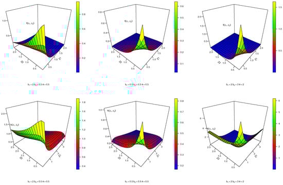
Figure 2. Joint pdf and joint hazard rate of CBKM-Ex distribution.

4.2.2. CBKM-Weibull (CBKM-W) Distribution

Obtaining the KM-Weibull (KM-W) distribution involves using the KM transformation and Weibull distribution. This allows us to obtain the cdf, pdf, and sf of the CBKM-W distribution (for $z_j>0,b_j>0$ and $a_j>0$ ) as follows:

$$\begin{array}{cc}\hfill F_{CBKM-W}(z_1,z_2)=& {\left\{{\left[\frac{e}{e-1}{\varpi }_1(z_1,b_1,a_1)\right]}^{-\theta }+{\left[\frac{e}{e-1}{\varpi }_2(z_2,b_2,a_2)\right]}^{-\theta }-1\right\}}^{-\frac{1}{\theta }},\hfill \end{array}$$

(54)

$$\begin{array}{cccc}\hfill f_{CBKM-W}(z_1,z_2)& ={\left[\frac{e}{e-1}\right]}^{-2\theta }{a}_1{b}_1^{a_1}{z}_1^{a_1-1}{e}^{-{\left(b_1{z}_1\right)}^{a_1}}{a}_2{b}_2^{a_2}{z}_2^{a_2-1}{e}^{-{\left(b_2{z}_2\right)}^{a_2}}\hfill & \hfill & \hfill \\ \hfill & e^{e^{-{\left(b_1{z}_1\right)}_1^a}+e^{-{\left(b_2{z}_2\right)}^{a_2}}-2}(1+\theta ){\left\{{\varpi }_1(z_1,b_1,a_1){\varpi }_2(z_2,b_2,a_2)\right\}}^{-1-\theta }\hfill & \hfill & \hfill \\ \hfill & {\left\{{\left[\frac{e}{e-1}{\varpi }_1(z_1,b_1,a_1)\right]}^{-\theta }+{\left[\frac{e}{e-1}{\varpi }_2(z_2,b_2,a_2)\right]}^{-\theta }-1\right\}}^{-2-\frac{1}{\theta }}.\hfill \end{array}$$

(55)

4.2.3. CBKM-Pareto (CBKM-Pa) Distribution

Obtaining the KM-Pareto (KM-Pa) distribution involves using the KM transformation and Pareto distribution. This allows us to obtain the cdf, pdf, and sf of the CBKM-Pa distribution (for $z_j>0$ and $v_j>0$) as follows:

$$\begin{array}{cc}\hfill F_{CBKM-Pa}(z_1,z_2)=& {\left\{{\left[\frac{e}{e-1}{\varpi }_1(z_1,v_1)\right]}^{-\theta }+{\left[\frac{e}{e-1}{\varpi }_2(z_2,v_2)\right]}^{-\theta }-1\right\}}^{-\frac{1}{\theta }},\hfill \end{array}$$

(56)

$$\begin{array}{cc}\hfill f_{CBKM-Pa}(z_1,z_2)=& {\left[\frac{e}{e-1}\right]}^{-2\theta }{v}_1{(1+z_1)}^{-(1+v_1)}{v}_2{(1+z_2)}^{-(1+v_2)}\hfill \\ \hfill & e^{{(1+z_1)}^{-v_1}+{(1+z_2)}^{-v_2}-2}(1+\theta ){\left\{{\varpi }_1(z_1,v_1){\varpi }_2(z_2,v_2)\right\}}^{-1-\theta }\hfill \\ \hfill & {\left\{{\left[\frac{e}{e-1}{\varpi }_1(z_1,v_1)\right]}^{-\theta }+{\left[\frac{e}{e-1}{\varpi }_2(z_2,v_2)\right]}^{-\theta }-1\right\}}^{-2-\frac{1}{\theta }}.\hfill \end{array}$$

(57)

4.3. Statistical Properties of the CBKM-T Family

In this section, we delve into a detailed examination of the statistical properties of the CBKM-T family, which are mathematically described by Equations (46) and (47). Specifically, we discuss various important characteristics of this model, including the marginal distributions, conditional distribution and generating random variables.

4.3.1. The Marginal Distributions

The marginal distributions of $Z_1$ and $Z_2$ in the joint Clayton BKM-T family’s pdf, as expressed by Equation (47), are not KM-T family marginals and are provided as

$$\begin{array}{cc}\hfill f_{Z_1,Clayton}(z_1,{\mathsf{\Lambda }}_1)=& \left[\frac{e}{e-1}\right]g(z_1;{\mathsf{\Lambda }}_1)e^{-G(z_1;{\mathsf{\Lambda }}_1)}\hfill \\ \hfill & \left[1-F_1^{-1-\theta }(z_1,{\mathsf{\Lambda }}_1){\left(F_1^{-\theta }(z_1,{\mathsf{\Lambda }}_1)-1\right)}^{-1-\frac{1}{\theta }}\right],\theta >0,\hfill \end{array}$$

(58)

and

$$\begin{array}{cc}\hfill f_{Z_2,Clayton}(z_2,{\mathsf{\Lambda }}_2)=& \left[\frac{e}{e-1}\right]g(z_2;{\mathsf{\Lambda }}_2)e^{-G(z_2;{\mathsf{\Lambda }}_2)}\hfill \\ \hfill & \left[1-F_2^{-1-\theta }(z_2,{\mathsf{\Lambda }}_2){\left(F_2^{-\theta }(z_2,{\mathsf{\Lambda }}_2)-1\right)}^{-1-\frac{1}{\theta }}\right],\theta >0.\hfill \end{array}$$

(59)

4.3.2. Conditional Distribution

For $l\ne j$ with $l,j=1,2$, we have the following:

(i)

The conditional probability distribution of $Z_l$ given $Z_j=z_j$ is

$$\begin{array}{cccc}\hfill f_{Z_l\mid Z_j,Clayton}(z_l\mid z_j)=& \left[\frac{e}{e-1}\right]g(z_l;{\mathsf{\Lambda }}_l)e^{-G(z_l;{\mathsf{\Lambda }}_l)}\hfill & \hfill & \\ & (1+\theta ){\left\{F_l(z_l,{\mathsf{\Lambda }}_l)F_j(z_j,{\mathsf{\Lambda }}_j)\right\}}^{-1-\theta }{\left\{F_l^{-\theta }(z_l,{\mathsf{\Lambda }}_l)+F_j^{-\theta }(z_j,{\mathsf{\Lambda }}_j)-1\right\}}^{-2-\frac{1}{\theta }}.\hfill \end{array}$$

(60)

(ii)

The conditional cdf of $Z_l$ given $Z_j=z_j$ is

$$\begin{array}{cc}\hfill F_{Z_l\mid Z_j,Clayton}(z_l\mid z_j)& =P(Z_l\le z_l\mid Z_j=z_j)\hfill \\ \hfill & ={\left\{F_j(z_j,{\mathsf{\Lambda }}_j)\right\}}^{-1-\theta }\left\{{\left[F_l^{-\theta }(z_l,{\mathsf{\Lambda }}_l)+F_j^{-\theta }(z_j,{\mathsf{\Lambda }}_j)-1\right]}^{-1-\frac{1}{\theta }}\right.\hfill \\ \hfill & \left.-{\left[F_j^{-\theta }(z_j,{\mathsf{\Lambda }}_j)-1\right]}^{-1-\frac{1}{\theta }}\right\}.\hfill \end{array}$$

(61)

(iii)

The conditional survival of $Z_l$ given $Z_j=z_j$ is

$$\begin{array}{cc}\hfill R_{Z_l\mid Z_j,Clayton}(z_l\mid z_j)& =P(Z_l>z_l\mid Z_j=z_j)\hfill \\ & =1-\left\{F_j^{-1-\theta }(z_j,{\mathsf{\Lambda }}_j){\left[F_l^{-\theta }(z_l,{\mathsf{\Lambda }}_l)+F_j^{-\theta }(z_j,{\mathsf{\Lambda }}_j)-1\right]}^{-1-\frac{1}{\theta }}\right.\hfill \\ \hfill & \left.-{\left[F_j^{-\theta }(z_j,{\mathsf{\Lambda }}_j)-1\right]}^{-1-\frac{1}{\theta }}\right\}.\hfill \end{array}$$

(62)

4.3.3. Generating Random Variables

A bivariate sample of the CBKM-T family based on the conditional method (61) can be generated:

(1)

Generate V and U independently from a uniform$(0,1)$ distribution.

(2)

Set $z_1=Q_{CBMK-T}=G^{-1}\left\{-log\left[1-\frac{(e-1)U}{e}\right]\right\}$.

(3)

$F_{Z_2\mid Z_1,Clayton}(z_2\mid z_1)=U$ in (61) to obtain $z_2$ using numerical analysis, such as Newton–Raphson, etc.

(4)

Repeat 1–3 (n) times to obtain $(z_{1i},z_{2i})$, $i=1,2,\dots ,n$.

5. Dependence Measures for FGMBKM-T Family and CBKM-T Family

In this section, we introduce some measures of dependence based on copulas for the FGMBKM-T family and CBKM-T family, such as Kendall’s tau (${\tau }_c$), Blomqvist’s medial correlation coefficient ($b_c$) and Spearman’s footrule coefficient ${\delta }_c$, which are defined by Nelsen [24] and Popović [37].

5.1. Kendall’s Tau (${\tau }_c$)

The difference between the probabilities of concordance and discordance of $(X_1,X_2)$ and $(\widetilde{X_1},\widetilde{X_2})$ is denoted as Kendall’s tau (${\tau }_c$). For copula terms, Kendall’s (${\tau }_c$) is defined as

$${\tau }_c=4{\int }_0^1{\int }_0^{1}c\left\{u_1,u_2\right\}C\left\{u_1,u_2\right\}d{u}_{1}d{u}_2-1.$$

For the FGM copula with parameter $\theta$, Kendall’s tau is given by ${\tau }_{c_{\theta }}=\frac{2\theta }{9}$, indicating a moderate level of dependence. Specifically, ${\tau }_{c_{\theta }}$ ranges between $-\frac{2}{9}$ and $\frac{2}{9}$, with ${\tau }_{c_{\theta }}=-\frac{2}{9}$ corresponding to perfect negative dependence, ${\tau }_{c_{\theta }}=0$ indicating independence, and ${\tau }_{c_{\theta }}=\frac{2}{9}$ representing perfect positive dependence.

For the Clayton copula with parameter $\theta$, Kendall’s tau is given by ${\tau }_{c_{\theta }}=\frac{\theta }{\theta +2}$, with values ranging from 0 to 1. This indicates that as $\theta$ increases, the level of dependence between the variables increases as well.

5.2. Blomqvist’s Medial Correlation Coefficient $\left(b_c\right)$

Using population medians for $x_0$ and $y_0$, Blomqvist [38] proposed and studied a measure which is called the medial correlation coefficient, denoted as Blomqvist’s medial correlation coefficient $\left(b_c\right)$.

Blomqvist’s medial correlation coefficient at the middle or center of ${\mathbf{I}}^2$ is also called the Blomqvist Beta. For copula terms, Blomqvist’s medial correlation coefficient $\left(b_c\right)$ is defined as

$$b_c=4C\left(\frac{1}{2},\frac{1}{2}\right)-1.$$

In case of the FGM copula, Blomqvist’s medial correlation coefficient $\left(b_c\right)$ is $\frac{\theta }{4}$, and this means that $b_{c_{\theta }}\in [\frac{-1}{4},\frac{1}{4}]$.

In the case of the Clayton copula, Blomqvist’s medial correlation coefficient is $4{\left(2^{\theta +1}-1\right)}^{-\frac{1}{\theta }}-1$.

5.3. Spearman’s Footrule Coefficient (${\delta }_c$)

Bekrizadeh [39] and Bukovšek et al. [40] defined Spearman’s footrule coefficient for X and Y as

$${\delta }_c=6{\int }_0^{1}C\left[u_1,u_1\right]d{u}_1-2.$$

In case of FGM copula, Spearman’s footrule coefficient ${\delta }_c$ is $\frac{\theta }{5}$ and this means that ${\gamma }_{c_{\theta }}\in [\frac{-1}{5},\frac{1}{5}]$. In case of the Clayton copula, Spearman’s footrule coefficient is $\frac{1+2\theta }{1-\theta }$.

6. Parameter Estimation Methods

In this section, we introduce two methods for estimating the unknown parameters of the FGMBKM-T family and CBKM-T family of distributions: maximum likelihood estimation (MLE) and Bayesian estimation.

6.1. Maximum Likelihood Estimation

Consider a sample of size n, denoted by $(Z_{11},Z_{21}),\dots ,(Z_{1n},Z_{2n})$. The likelihood functions for the FGMBKM-T family and CBKM-T family of distributions with a vector of parameters $\Theta =({\mathsf{\Lambda }}_1,{\mathsf{\Lambda }}_2,\theta )$ based on FGM and Clayton copulas are given below.

The log-likelihood function $l(\Theta )$ for the FGMBKM-T family of distributions can be written as follows:

$$\begin{array}{cccc}\hfill l_{FGMBKM-T}(\Theta )=& 2n\left[1-ln\left(e-1\right)\right]+\sum _{i=1}^{n}lng(z_{1i},{\mathsf{\Lambda }}_1)+\sum _{i=1}^{n}lng(z_{2i},{\mathsf{\Lambda }}_2)\hfill & \hfill & \\ \hfill & -\sum _{i=1}^{n}G(z_{1i};{\mathsf{\Lambda }}_1)-\sum _{i=1}^{n}G(z_{2i};{\mathsf{\Lambda }}_2)\hfill & \hfill & \\ \hfill & +\sum _{i=1}^{n}ln\left\{1+\theta \left[1-\frac{2e}{e-1}{\varpi }_{1i}(z_{1i},{\mathsf{\Lambda }}_1)\right]\left[1-\frac{2e}{e-1}{\varpi }_{2i}(z_{2i},{\mathsf{\Lambda }}_2)\right]\right\},\hfill \end{array}$$

(63)

where ${\varpi }_{ji}(x_{ji},{\mathsf{\Lambda }}_j)=\left(1-e^{-G(x_{ji};{\mathsf{\Lambda }}_j)}\right)$. The log-likelihood function $l(\Theta )$ for the CBKM-T family of distributions can be written as follows:

$$\begin{array}{cccc}\hfill l_{CBKM-T}(\Theta )=& -2n\theta \left[1-ln\left(e-1\right)\right]+\sum _{i=1}^{n}lng(z_{1i},{\mathsf{\Lambda }}_1)+\sum _{i=1}^{n}lng(z_{2i},{\mathsf{\Lambda }}_2)\hfill & \hfill & \\ \hfill & -\sum _{i=1}^{n}G(z_{1i};{\mathsf{\Lambda }}_1)-\sum _{i=1}^{n}G(z_{2i};{\mathsf{\Lambda }}_2)+nln\left(1+\theta \right)\hfill & \hfill & \\ \hfill & -\left(1+\theta \right)\sum _{i=1}^{n}ln\left[{\varpi }_{1i}(z_{1i},{\mathsf{\Lambda }}_1){\varpi }_{2i}(z_{2i},{\mathsf{\Lambda }}_2)\right]\hfill & \hfill & \\ \hfill & -\left(2+\frac{1}{\theta }\right)\sum _{i=1}^{n}ln\left\{{\left[\frac{e}{e-1}{\varpi }_{1i}(z_{1i},{\mathsf{\Lambda }}_1)\right]}^{-\theta }+{\left[\frac{e}{e-1}{\varpi }_{2i}(z_{2i},{\mathsf{\Lambda }}_2)\right]}^{-\theta }-1\right\}.\hfill \end{array}$$

(64)

The first partial derivatives of Equation (63) with respect to ${\mathsf{\Lambda }}_1,{\mathsf{\Lambda }}_2$, and $\theta$ can be expressed as

$$\begin{array}{cccc}\hfill \frac{\partial l_{FGMBKM-T}(\Theta )}{\partial {\mathsf{\Lambda }}_j}=& \sum _{i=1}^n\frac{\varphi (z_{ji},{\mathsf{\Lambda }}_j)}{g(z_{ji},{\mathsf{\Lambda }}_j)}-\sum _{i=1}^n\mathsf{\Phi }(z_{ji};{\mathsf{\Lambda }}_j)\hfill & \hfill & \\ \hfill & -\sum _{i=1}^n\frac{\frac{2\theta e}{e-1}\left[1-\frac{2e}{e-1}{\varpi }_{li}(z_{li};{\mathsf{\Lambda }}_l)\right]e^{-G\left(z_{ji,\mathsf{\Lambda }}\right)}\mathsf{\Phi }(z_{ji};{\mathsf{\Lambda }}_j)}{1+\theta \left[1-\frac{2e}{e-1}{\varpi }_{1i}(z_{1i};{\mathsf{\Lambda }}_1)\right]\left[1-\frac{2e}{e-1}{\varpi }_{2i}(z_{2i};{\mathsf{\Lambda }}_2)\right]},\hfill & \hfill \end{array}$$

(65)

$$\frac{\partial l_{FGMBKM-T}(\Theta )}{\partial \theta }=\sum _{i=1}^n\frac{\left[1-\frac{2e}{e-1}{\varpi }_{1i}(z_{1i};{\mathsf{\Lambda }}_1)\right]\left[1-\frac{2e}{e-1}{\varpi }_{2i}(z_{2i};{\mathsf{\Lambda }}_2)\right])}{1+\theta \left[1-\frac{2e}{e-1}{\varpi }_{1i}(z_{1i};{\mathsf{\Lambda }}_1)\right]\left[1-\frac{2e}{e-1}{\varpi }_{2i}(z_{2i};{\mathsf{\Lambda }}_2)\right]},$$

(66)

where $\varphi (z_{ji};{\mathsf{\Lambda }}_j)=\frac{\partial g(z_{ji};{\mathsf{\Lambda }}_j)}{\partial {\mathsf{\Lambda }}_j}$, $\mathsf{\Phi }(z_{ji};{\mathsf{\Lambda }}_j)=\frac{\partial G(z_{ji};{\mathsf{\Lambda }}_j)}{\partial {\mathsf{\Lambda }}_j}$ and $j=(1,2)$, $l=(1,2)$; $j\ne l,$ (for example $j=1$ then $l=2)$.

The first partial derivatives of Equation (64) with respect to ${\mathsf{\Lambda }}_1,{\mathsf{\Lambda }}_2$, and $\theta$ can be expressed as

$$\begin{array}{cccc}\hfill \frac{\partial l_{CBKM-T}(\Theta )}{\partial {\mathsf{\Lambda }}_j}=& \sum _{i=1}^n\frac{\varphi (z_{ji},{\mathsf{\Lambda }}_j)}{g(z_{ji},{\mathsf{\Lambda }}_j)}-\sum _{i=1}^n\mathsf{\Phi }(z_{ji};{\mathsf{\Lambda }}_j)\hfill & \hfill & \\ \hfill & -(1+\theta )\sum _{i=1}^n\frac{{\varpi }_{li}(z_{li};{\mathsf{\Lambda }}_l)e^{-G\left(z_{ji,\mathsf{\Lambda }}\right)}\mathsf{\Phi }(z_{ji};{\mathsf{\Lambda }}_j)}{{\varpi }_{1i}(z_{1i};{\mathsf{\Lambda }}_1){\varpi }_{2i}(z_{2i};{\mathsf{\Lambda }}_2)}\hfill & \hfill & \\ \hfill & +\left(2+\frac{1}{\theta }\right)\sum _{i=1}^n\frac{\frac{\theta e}{e-1}{\left[\frac{e}{e-1}{\varpi }_{ji}(z_{ji};{\mathsf{\Lambda }}_j)\right]}^{-\theta -1}{e}^{-G\left(z_{ji,\mathsf{\Lambda }}\right)}\mathsf{\Phi }(z_{ji};{\mathsf{\Lambda }}_j)}{{\left[\frac{e}{e-1}{\varpi }_{1i}(z_{1i};{\mathsf{\Lambda }}_1)\right]}^{-\theta }+{\left[\frac{e}{e-1}{\varpi }_{2i}(z_{2i};{\mathsf{\Lambda }}_2)\right]}^{-\theta }-1},\hfill & \hfill \end{array}$$

(67)

$$\begin{array}{cccc}\hfill \frac{\partial l_{CBKM-T}(\Theta )}{\partial \theta }=& -2n\left[1-ln\left(e-1\right)\right]+\frac{n}{1+\theta }-\sum _{i=1}^{n}ln\left[{\varpi }_{1i}(z_{1i},{\mathsf{\Lambda }}_1){\varpi }_{2i}(z_{2i},{\mathsf{\Lambda }}_2)\right]\hfill & \hfill & \\ \hfill & +\left(2+\frac{1}{\theta }\right)\sum _{i=1}^n\left\{\frac{{\left[\frac{e}{e-1}{\varpi }_{1i}(z_{1i};{\mathsf{\Lambda }}_1)\right]}^{-\theta }\left[ln\frac{e}{e-1}+ln{\varpi }_{1i}(z_{1i};{\mathsf{\Lambda }}_1)\right]}{{\left[\frac{e}{e-1}{\varpi }_{1i}(z_{1i};{\mathsf{\Lambda }}_1)\right]}^{-\theta }+{\left[\frac{e}{e-1}{\varpi }_{2i}(z_{2i};{\mathsf{\Lambda }}_2)\right]}^{-\theta }-1}\right.\hfill \\ \hfill & \left.+\frac{{\left[\frac{e}{e-1}{\varpi }_{2i}(z_{2i};{\mathsf{\Lambda }}_2)\right]}^{-\theta }\left[ln\frac{e}{e-1}+ln{\varpi }_{2i}(z_{2i};{\mathsf{\Lambda }}_2)\right]}{{\left[\frac{e}{e-1}{\varpi }_{1i}(z_{1i};{\mathsf{\Lambda }}_1)\right]}^{-\theta }+{\left[\frac{e}{e-1}{\varpi }_{2i}(z_{2i};{\mathsf{\Lambda }}_2)\right]}^{-\theta }-1}\right\}\hfill & \hfill & \\ \hfill & +\frac{1}{{\theta }^2}\sum _{i=1}^{n}ln\left\{{\left[\frac{e}{e-1}{\varpi }_{1i}(z_{1i},{\mathsf{\Lambda }}_1)\right]}^{-\theta }+{\left[\frac{e}{e-1}{\varpi }_{2i}(z_{2i},{\mathsf{\Lambda }}_2)\right]}^{-\theta }-1\right\}.\hfill \end{array}$$

By equating Equations (65)–(67) by zeros, we obtain the non-linear normal equations. So, the solution has to be obtained numerically.

6.2. Bayesian Estimation

The Bayes estimators and related HPD intervals of ${\mathsf{\Lambda }}_1,{\mathsf{\Lambda }}_2$, and $\theta$ are developed in this section based on the SE loss function. If ${\mathsf{\Lambda }}_1,{\mathsf{\Lambda }}_2>0$, then the gamma priors $Gamma(a_1,c_1),Gamma(a_2,c_2)$ are assumed to be separately distributed for parameters ${\mathsf{\Lambda }}_1$ and ${\mathsf{\Lambda }}_2$ in the FGMBKM-Ex and CBKM-Ex models, respectively. Consider gamma priors for the following reasons, among others:

• Based on hyper-parameter values, they offer a variety of shapes.
• They have an adaptable disposition.
• They are reasonably simple, succinct, and might not produce a result with a complex estimate problem.

So, ${\beta }_1$ and ${\beta }_2$ joint prior density is

$$\pi \left({\beta }_1,{\beta }_2\right)\propto {\beta }_1^{a_1-1}{\beta }_2^{a_2-1}{e}^{-c_1{\beta }_1-c_2{\beta }_2},a_1,a_2>0,c_1,c_2>0,$$

(68)

where the hyper-parameters $a_i$ and $c_i,i=1,2$ are the ones that hold the previous knowledge.

Many writers created Bayesian estimates for their parameter models, utilizing instructive gamma priors, including Kundu and Howlader [41], Dey and Dey [42], Dey et al. [43], and Dey et al. [44]. For the FGM copula, parameter $\theta$ is uniform from −1 to 1. For the Clayton copula, parameter $\theta$ has gamma prior distribution $Gamma(a_3,c_3)$.

The likelihood function and the prior Equation (68) can be combined to provide the posterior distribution of ${\beta }_1$ and ${\beta }_2$, which are defined and written as

$${\pi }^{*}({\beta }_1,{\beta }_2,\theta |data)=\frac{L({\beta }_1,{\beta }_2,\theta |data)\pi ({\beta }_1,{\beta }_2)\pi \left(\theta \right)}{\underset{0}{\overset{\infty }{\int }}\underset{0}{\overset{\infty }{\int }}\underset{0}{\overset{\infty }{\int }}L({\beta }_1,{\beta }_2,\theta |data)\pi ({\beta }_1,{\beta }_2)\pi \left(\theta \right)d{\beta }_{1}d{\beta }_{2}d\theta }.$$

(69)

A square error loss (SEL) function, which is a commonly used function, is a symmetric loss function, defined as

$$L(\varphi ,\hat{\varphi })=(\hat{\varphi }-\varphi ),$$

(70)

where $\hat{\varphi }$ is an estimate of $\varphi$.

The Bayes estimate of any function of ${\beta }_1,{\beta }_2$ and $\theta$, say, $g\left(\alpha ,\beta ,\beta \right)$ under the SEL function, can be determined as

$${\hat{g}}_{BS}\left({\beta }_1,{\beta }_2,\theta |x\right)=E_{{\beta }_1,{\beta }_2,\theta |x}\left(g\left({\beta }_1,{\beta }_2,\theta \right)\right),$$

(71)

where

$$E_{{\beta }_1,{\beta }_2,\theta |data}\left(g\left({\beta }_1,{\beta }_2,\theta \right)\right)=\frac{\underset{0}{\overset{\infty }{\int }}\underset{0}{\overset{\infty }{\int }}\underset{0}{\overset{\infty }{\int }}g\left({\beta }_1,{\beta }_2,\theta \right){\pi }_1\left({\beta }_1\right){\pi }_2\left({\beta }_2\right){\pi }_3\left(\theta \right)L({\beta }_1,{\beta }_2,\theta |data)d{\beta }_{1}d{\beta }_{2}d\theta }{\underset{0}{\overset{\infty }{\int }}\underset{0}{\overset{\infty }{\int }}\underset{0}{\overset{\infty }{\int }}{\pi }_1\left({\beta }_1\right){\pi }_2\left({\beta }_2\right){\pi }_3\left(\theta \right)L({\beta }_1,{\beta }_2,\theta |data)d{\beta }_{1}d{\beta }_{2}d\theta }.$$

(72)

It is noted that an explicit form cannot be produced for the ratio of the numerous integrals in Equation (72). So, the iterative algorithm should be used as MCMC.

To generate samples for the joint posterior function in Equation (69), MCMC was created. The estimation of an integral value is the main focus of the MCMC mechanism. In order to implement the MCMC method, we take into account the Gibbs in the Metropolis Hasting sampler approach. The joint posterior distribution for FGMBKM-Ex and CBKM-Ex can be represented as

$$\begin{array}{cccc}\hfill \mathsf{\Pi }({\beta }_1,{\beta }_2,\theta |z_1,z_2)\propto & {\beta }_1^{a_1-1}{\beta }_2^{a_2-1}{e}^{-c_1{\beta }_1-c_2{\beta }_2}g(z_1;{\beta }_1)g(z_2;{\beta }_2)e^{-G(z_1;{\beta }_1)-G(z_2,{\beta }_2)}\hfill & \hfill & \\ \hfill & \left\{1+\theta \left[1-\frac{2e}{e-1}\left(1-e^{-G(z_1;{\beta }_1)}\right)\right]\left[1-\frac{2e}{e-1}\left(1-e^{-G(z_2;{\beta }_2)}\right)\right]\right\},\hfill \end{array}$$

(73)

$$\begin{array}{cccc}\hfill \mathsf{\Pi }({\beta }_1,{\beta }_2,\theta |z_1,z_2)\propto & {\beta }_1^{a_1-1}{\beta }_2^{a_2-1}{\theta }^{a_3-1}{\left[\frac{e}{e-1}\right]}^{-2\theta }g(z_1;{\beta }_1)g(z_2;{\beta }_2)e^{-G(z_1;{\beta }_1)-G(z_2,{\beta }_2)}(1+\theta )\hfill & \hfill & \\ \hfill & e^{-c_1{\beta }_1-c_2{\beta }_2-c_3\theta }{\left\{\left(1-e^{-G(z_1;{\beta }_1)}\right)\left(1-e^{-G(z_2;{\beta }_2)}\right)\right\}}^{-1-\theta }\hfill & \hfill & \\ \hfill & {\left\{{\left[\frac{e}{e-1}\left(1-e^{-G(z_1;{\beta }_1)}\right)\right]}^{-\theta }+{\left[\frac{e}{e-1}\left(1-e^{-G(z_2;{\beta }_2)}\right)\right]}^{-\theta }-1\right\}}^{-2-\frac{1}{\theta }},\hfill \end{array}$$

(74)

respectively.

7. Confidence Intervals

This section presents two distinct techniques for creating confidence intervals (CI) for the unknown parameters of the FGMBKM-T family and CBKM-T family. These methods include the asymptotic confidence interval (ACI) and the bootstrap confidence interval, which is further categorized into percentile bootstrap and bootstrap-t for ${\mathsf{\Lambda }}_j$, where $j=1,2$ and $\theta$.

7.1. Asymptotic Confidence Intervals

One of the most widely used approaches for establishing confidence intervals for parameters involves utilizing the asymptotic normality of the maximum likelihood estimator (MLE). Specifically, this involves the asymptotic variance–covariance matrix of the MLE of the parameters, which is referred to as the Fisher information matrix $I(\Theta )$. This matrix is derived from the negative second derivatives of the natural logarithm of the likelihood function, which is evaluated at the estimated parameter values $\hat{\Theta }=(\widehat{{\mathsf{\Lambda }}_1},\widehat{{\mathsf{\Lambda }}_2},\hat{\theta })$. The asymptotic variance–covariance matrix of the parameter vector $\Theta$ can be represented as

$$I\left(\hat{\Theta }\right)=-\left[\begin{array}{ccc}{I}_{\widehat{{\mathsf{\Lambda }}_1}\widehat{{\mathsf{\Lambda }}_1}}& & \\ I_{\widehat{{\mathsf{\Lambda }}_2}\widehat{{\mathsf{\Lambda }}_1}}& I_{\widehat{{\mathsf{\Lambda }}_2}\widehat{{\mathsf{\Lambda }}_2}}& \\ I_{\hat{\theta }\widehat{{\mathsf{\Lambda }}_1}}& I_{\hat{\theta }\widehat{{\mathsf{\Lambda }}_2}}& I_{\hat{\theta }\hat{\theta }},\end{array}\right]$$

(75)

where $V\left(\hat{\Theta }\right)=I^{-1}\left(\hat{\Theta }\right)$. Confidence intervals for parameter $\Theta$ can be constructed based on the asymptotic normality of the MLE. Specifically, a $100(1-\alpha )\%$ confidence interval for parameter $\Theta$ can be constructed as $\widehat{{\mathsf{\Lambda }}_l}\pm Z_{0.025}\sqrt{I_{\widehat{{\mathsf{\Lambda }}_l}\widehat{{\mathsf{\Lambda }}_l}}}$ and $\hat{\theta }\pm Z_{0.025}\sqrt{I_{\hat{\theta }\hat{\theta }}}$, where $l=1,2$ and $Z_{0.025}$ represents the percentile of the standard normal distribution with a right tail probability of $\frac{\alpha }{2}$.

7.2. Bootstrap Confidence Interval

The bootstrap is a statistical inference technique based on resampling. Its common application is in the estimation of confidence intervals. For further details, refer to Efron [45]. In this subsection, we employ the parametric bootstrap approach to establish confidence intervals for the unknown parameters ${\mathsf{\Lambda }}_j$, where $j=1,2$, and $\theta$. We present two parametric bootstrap methods, namely, the percentile bootstrap (B-P) and the bootstrap-t (B-t) CI.

7.2.1. Percentile Bootstrap Confidence Interval

(1)

Determine the maximum likelihood estimator (MLE) or Bayesian estimator for the FGMBKM-T and CBKM-T distributions.

(2)

Use the values of ${\mathsf{\Lambda }}_j$ and $\theta$ to generate a set of bootstrap samples, from which you can estimate the bootstrap values of ${\mathsf{\Lambda }}_j$ (denoted as ${\mathsf{\Lambda }}_j^b$) and $\theta$ (denoted as ${\theta }^b$).

(3)

Repeat step (2) B times to obtain B sets of bootstrap estimates for ${\mathsf{\Lambda }}_j$ and $\theta$.

(4)

Arrange the B sets of bootstrap estimates for ${\mathsf{\Lambda }}_j$ and $\theta$ in ascending order and denote them as (${\mathsf{\Lambda }}_j^{b\left[1\right]}$, ${\mathsf{\Lambda }}_j^{b\left[2\right]}$, …, ${\mathsf{\Lambda }}_j^{b\left[B\right]}$) and (${\theta }^{b\left[1\right]}$, ${\theta }^{b\left[2\right]}$, …, ${\theta }^{b\left[B\right]}$), respectively.

(5)

Compute the two-sided 100(1 − $\gamma$)% percentile bootstrap confidence interval for each of the unknown parameters ${\mathsf{\Lambda }}_j$ (where $j=1,2$) and $\theta$ using the bootstrap estimates obtained in step (4). These intervals are given by [${\mathsf{\Lambda }}_j^{b\left(\left[B\frac{\gamma }{2}\right]\right)}$, ${\mathsf{\Lambda }}_j^{b\left(\left[B(1-\frac{\gamma }{2})\right]\right)}$] and [${\theta }^{b\left(\left[B\frac{\gamma }{2}\right]\right)}$, ${\theta }^{b\left(\left[B(1-\frac{\gamma }{2})\right]\right)}$], respectively.

7.2.2. Bootstrap-t Confidence Interval

(1)

Perform the same steps (1,2) as in the Boot-p method.

(2)

Calculate the t-statistic of the estimator $\Theta$ using $T=\frac{{\hat{\Theta }}^b-\hat{\Theta }}{\sqrt{V\left({\hat{\Theta }}^b\right)}}$, where $V\left({\hat{\Theta }}^b\right)$ is the asymptotic variance of ${\hat{\Theta }}^b$ that can be obtained using the Fisher information matrix.

(3)

Repeat the above step B times and obtain ($T^{\left(1\right)},T^{\left(2\right)},\dots ,T^{\left(B\right)}$).

(4)

Arrange the values of T obtained in step 3 in ascending order as $(T^{\left[1\right]},T^{\left[2\right]},\dots ,T^{\left[B\right]})$.

(5)

Compute a two-sided bootstrap confidence interval for the unknown parameters ${\mathsf{\Lambda }}_j$ and $\theta$. For ${\mathsf{\Lambda }}_j$, where $j=1,2$, the interval is given by [${\mathsf{\Lambda }}_j+T_j^{b\left(\left[B\frac{\gamma }{2}\right]\right)}\sqrt{V({\mathsf{\Lambda }}_j^b}),{\mathsf{\Lambda }}_j+\sqrt{V({\mathsf{\Lambda }}_j^b})T_j^{b\left(\left[B(1-\frac{\gamma }{2})\right]\right)}$]. For $\theta$, the interval is given by [$\theta +T_j^{b\left(\left[B\frac{\gamma }{2}\right]\right)}\sqrt{V({\theta }^b}),$$\theta +\sqrt{V({\theta }^b})T_j^{b\left(\left[B(1-\frac{\gamma }{2})\right]\right)}$]. Here, $\gamma$ is the confidence level specified by the user.

8. Simulation

To evaluate the effectiveness of the MLE and Bayesian utilized for the estimate of FGMBKM-Ex and CBKM-Ex parameters, a simulation exercise was carried out. The simulation was carried out in accordance with the following steps:

• The FGMBKM-Ex and CBKM-Ex models were used to produce 1000 data-sets, each corresponding to a size of 40, 100 or 150. We generated 1000 FGMBKM-Ex and CBKM-Ex samples for different combinations. For the FGMBKM-Ex and CBKM-Ex models with varied positive and negative correlations between the four theoretical parameters, we have the following:

  –

  ${\beta }_1=0.3,{\beta }_2=0.5$ and $\theta =-0.5$

  –

  ${\beta }_1=0.8,{\beta }_2=0.5$ and $\theta =-0.5$

  –

  ${\beta }_1=1.5,{\beta }_2=0.5$ and $\theta =-0.5$

  –

  ${\beta }_1=3,{\beta }_2=0.5$ and $\theta =-0.5$

  –

  ${\beta }_1=0.3,{\beta }_2=2$ and $\theta =0.6$

  –

  ${\beta }_1=0.8,{\beta }_2=2$ and $\theta =0.6$

  –

  ${\beta }_1=1.5,{\beta }_2=2$ and $\theta =0.6$

  –

  ${\beta }_1=3,{\beta }_2=2$ and $\theta =0.6$

  For the FGMBKM-Ex and CBKM-Ex models with varied positive correlation between the eight theoretical parameters, we have the following:

  –

  ${\beta }_1=0.3,{\beta }_2=0.5$ and $\theta =0.6$

  –

  ${\beta }_1=0.8,{\beta }_2=0.5$ and $\theta =0.6$

  –

  ${\beta }_1=1.5,{\beta }_2=0.5$ and $\theta =0.6$

  –

  ${\beta }_1=3,{\beta }_2=0.5$ and $\theta =0.6$

  –

  ${\beta }_1=0.3,{\beta }_2=2$ and $\theta =1.5$

  –

  ${\beta }_1=0.8,{\beta }_2=2$ and $\theta =1.5$

  –

  ${\beta }_1=1.5,{\beta }_2=2$ and $\theta =1.5$

  –

  ${\beta }_1=3,{\beta }_2=2$ and $\theta =1.5$

• A general form to generate x from one marginal $g(z_1;{\beta }_1)$ and then simulate a corresponding bivariate vector using the conditional density is $G\left(z_2\right|z_1)$. See Section 3.3.3 and Section 4.3.3.
• For each model taken into consideration, the bias, mean square error (MSE), length of confidence intervals (LCI), and coverage probability (CP) were determined.
• All necessary numerical calculations were carried out using the R 4.3.0 statistical programming language software, primarily three helpful statistical packages, namely:

  –

  “copula” for carrying out the computations of the dependency measures proposed.

  –

  “coda” for carrying out the computations of the MCMC Bayesian proposed.

  –

  “maxLik” for using the Newton–Raphson method of maximization in the computations, proposed.

• The performance of the MLE approach and the Bayesian utilized for the estimate of the FGMBKM-Ex and CBKM-Ex model parameters, accounting for MSE and bias relevant to the examples described in Step 1 of the simulation research, is displayed in Table A1, Table A2, Table A3 and Table A4 below.
• Based on their average asymptotic LCI (AALCI) and coverage percentages (CP), the interval estimates of ${\beta }_1,{\beta }_2$, and $\theta$ were compared. To obtain Bayesian interval estimates, the HPD was used. The level of confidence intervals is 95%.

The most important findings from the simulation study as presented in Table A1, Table A2, Table A3 and Table A4 of Appendix A, can be summarized in the following points:

• The MSE, bias, and LCI on the estimated parameters of the FGMBKM-Ex and CBKM-Ex models decrease as the sample size grows, but the CP increases.
• Overall, the results show that the Bayesian technique outperforms the ML when accounting for the MSE in estimating positive and negative relationships (FGMBKM-Ex and CBKM-Ex).
• The MSE, bias, and LCI of each suggested estimate behave satisfactorily as n is increased.
• When ${\beta }_1$ increases, the MSE, bias, and LCI of each suggested estimate increases.
• When ${\beta }_2$ increases, the MSE, bias, and LCI of each suggested estimate increases.
• When $\theta$ increases, the MSE, bias, and LCI of each suggested estimate increases.

9. Application of Real Data

In this section, we explore two real-world data examples: the kidney patient data-set, which serves as the motivation for our research, and the football data-set. We employ the FGMBKM-T family and CBKM-T family of distributions to model these data-sets. To assess the goodness of fit, we apply a suitable measure. Point estimations are performed numerically using the appropriate R-codes. Firstly, 30 patients’ worth of data were collected by McGilchrist and Aisbett in [46].

The recurring infection issue among kidney patients utilizing portable dialysis machines is addressed in this study. Specifically, the infections manifest at the catheter insertion site, necessitating catheter removal, infection treatment, and subsequent catheter reinsertion. The recurrence times refer to the intervals between catheter insertions and subsequent infections.

Assume x1 and x2 are the first and second recurrence times, respectively:

x1: 8, 23, 22, 447, 30, 24, 7, 511, 53, 15, 7, 141, 96, 149, 536, 152, 402, 13, 39, 12, 113, 132, 34, 2, 130, 17, 185, 292, 22, 15.

x2: 16, 13, 28, 318, 12, 245, 9, 30, 196, 154, 333, 8, 38, 70, 25, 362, 24, 66, 46, 40, 201, 156, 30, 25, 26, 4, 117, 114, 159, 108.

The data-set is presented in [46] by McGilchrist and Aisbett. This information shows how often infections return in kidney patients.

Secondly: We take into account a bivariate data-set on the UEFA Champions League group stage for the seasons 2004–2005 and 2005–2006. Only games with at least one goal scored by either team directly from a kick and at least one goal scored by the home team are taken into consideration; for more information, see Meintanis (2007). The first variable (W1) is the amount of time (in minutes) that has passed since any team has scored on a first kick, while the second one (W2) is the amount of time (in minutes) that has passed since the home side has scored on a first goal of any kind. To acquire information on the unit square (0, 1) (0, 1), the times are divided by 90 min (the length of the entire game).

Table 3 discusses data-set dependence measure (correlation) and goodness-of-fit test for FGM, AMH, and the Clayton copula function which can be used in the above model for each data-set. By analyzing the results, we observe that the FGM copula cannot be utilized for data II since the correlation in these data exceeds the threshold of $\frac{1}{3}$. This limitation arises from the fact that the FGM copula’s dependence parameter ($\theta$) is bounded between −1 and 1. It is important to note that the Spearman correlation for the FGM copula is determined by $\frac{\theta }{3}$. Hence, in order for the bivariate FGM distribution to be applicable, the correlation should lie within the range of $\frac{-1}{3}$ to $\frac{1}{3}$.

Table 3. Correlation and goodness of fit of copula function.

Data	Correlation		Clayton	FGM	AMH
I	0.0511	statistic	0.1442	0.2903	0.2114
		parameter	0.3033	0.4670	0.4975
		p-value	0.7628	0.3944	0.5487
II	0.3690	statistic	0.2846	Not Applying	0.4849
		parameter	0.6078		0.7888
		p-value	0.2384		0.1982

Figure 3 discusses the scatter plot with a boxplot for each data-set: the left discusses kidney patients’ data, while the right discusses the football data-set.

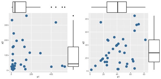
Figure 3. Scatter plot with boxplot.

Table 4 discusses the MLE estimates with different measures of each comparison model for kidney infection data, which indicates that the FGMBKM-W distribution is the best bivariate model to fit the kidney infection data-set, where the FGMBKM-W distribution has the lowest value of LL, AIC, CAIC, BIC, and HQIC compared to other bivariate copula models as FGM bivariate inverted Topp–Leone (FGMBITL) [15], Clayton bivariate inverted Topp–Leone (CBITL) [15], AMH bivariate Fréchet (AMHBF) [10], FGM bivariate Fréchet (FGMBF) [10], FGM bivariate Chen (FGMBC) [47], FGMC bivariate Weibull (FGMBW) [11], FGM bivariate generalized exponential (FGMBGE) [48], bivariate Burr X exponential (BBuXexp) [49] and FGM bivariate gamma (FGMBG) [50]. Figure 4 discusses the estimated joint pdf and joint hazard rate of FGMBKM-W distribution.

Table 4. MLE estimates with different measures of each comparison model for kidney infection data.

		${\mathit{\beta }}_1$	$\mathit{\alpha }1$	${\mathit{\beta }}_2$	${\mathit{\alpha }}_2$	$\mathit{\theta }$	LL	AIC	CAIC	BIC	HQIC
FGMBKM-Ex	estimates	0.0068		0.0078		0.3605	339.4979	684.9959	685.9189	689.1994	686.3406
	SE	0.0013		0.0016		0.4434
FGMBKM-W	estimates	0.0070	0.8100	0.0075	1.5765	0.3611	334.9842	679.9685	682.4685	686.9745	682.2098
	SE	0.0017	0.1108	0.0005	0.1304	0.2781
FGMBF	estimates	22.7765	0.7286	27.9028	0.8661	0.6119	340.7127	691.4254	693.9254	698.4313	693.6666
	SE	6.1354	0.0979	6.2964	0.1175	0.5613
AMHBF	estimates	23.0689	0.7266	28.1589	0.8638	0.5393	340.6412	691.2824	693.7824	698.2884	693.5237
	SE	6.1198	0.0978	6.2906	0.1171	0.3541
FGMBW	estimates	0.7513	99.9740	0.9291	95.4974	0.3992	338.9349	687.8698	690.3698	694.8758	690.1111
	SE	0.1053	25.6610	0.1322	19.8581	0.4987
FGMBGe	estimates	0.6660	0.0063	0.9258	0.0096	0.3775	339.5445	689.0890	691.5890	696.0950	691.3302
	SE	0.1485	0.0016	0.2174	0.0023	0.4848
FGMBG	estimates	0.6697	179.8593	0.9230	107.8414	0.3806	339.4889	688.9778	691.4778	695.9838	691.2191
	SE	0.1463	56.1853	0.2076	31.9672	0.4869
CBITL	estimates	0.3605		0.3409		3.0826	362.7520	731.5039	732.4270	735.7075	732.8487
	SE	0.0635		0.0601		0.9243
FGMBITL	estimates	0.3628		0.3523		0.4670	370.2663	746.5325	747.4556	750.7361	747.8773
	SE	0.0739		0.0397		1.0192
FGMBCH	estimates	0.0504	0.2336	0.0326	0.2651	0.3921	343.4072	696.8145	699.3145	703.8204	699.0557
	SE	0.0190	0.0168	0.0136	0.0181	0.5718
BBuXexp	estimates	0.0016	0.0548	0.0473	0.1021		373.7172	755.4343	757.0343	761.0391	757.2273
	SE	0.0002	0.0142	0.0116	0.0302
CBKM-Ex	estimates	0.0068		0.0076		0.2967	339.1936	684.3871	685.3102	688.5907	685.7319
	SE	0.0013		0.0015		0.2826
CBKM-W	estimates	0.0070	0.8179	0.0079	1.0046	0.4128	337.9455	685.8909	688.3909	692.8969	688.1322
	SE	0.0017	0.1121	0.0016	0.1410	0.3586

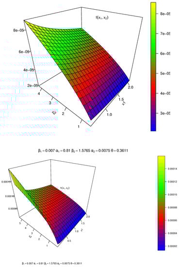
Figure 4. Joint pdf and joint hazard rate of FGMBKM-W.

Table 5 discusses the MLE estimates with different measures of each comparison model for the football data, which indicates that the CBKM-W distribution is the best bivariate model to fit the football data-set, where the CBKM-W distribution has the lowest value of LL, AIC, CAIC, BIC, and HQIC. Figure 5 discusses the estimated joint pdf and joint hazard rate of the CBKM-W distribution.

Table 5. MLE estimates with different measures of each comparison model for football data.

		${\mathit{\beta }}_1$	${\mathit{\alpha }}_1$	${\mathit{\beta }}_2$	${\mathit{\alpha }}_2$	$\mathit{\theta }$	LL	AIC	CAIC	BIC	HQIC
CBKM-Ex	estimates	0.0184		0.0271		0.4641	337.5242	681.0485	681.7757	685.8812	682.7522
	SE	0.0032		0.0047		0.5251
CBKM-W	estimates	0.0192	2.2996	0.0236	1.5194	0.3331	322.6669	655.3338	657.2693	663.3884	658.1734
	SE	0.0016	0.3058	0.0029	0.1930	0.2061
AMHBF	estimates	20.6832	0.9876	11.7831	0.9202	0.9914	351.0523	712.1046	714.0400	720.1591	714.9442
	SE	3.5265	0.1023	2.1454	0.1091	0.0170
CBITL	estimates	0.3437		0.4007		6.6079	378.3274	762.6548	763.3821	767.4876	764.3586
	SE	0.0609		0.0734		1.3010

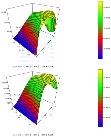
Figure 5. Joint pdf and joint hazard rate of CBKM-W.

10. Conclusions

In this paper, we emphasize the practical significance of the method introduced. The study introduces two innovative bivariate families, the FGMBKM-T family and CBKM-T family, which offer versatile applications in analyzing diverse data types, including medical- and sports-related data-sets. These families demonstrate efficacy in handling various statistical properties and provide valuable insights in different contexts. Additionally, we derive the bivariate KM-EX, KM-W, and KM-Pa distributions based on the FGM and Clayton copula functions. These distributions further expand the applicability of the proposed method and contribute to the advancement of bivariate modeling techniques. The FGMBKM-T and CBKM-T families, along with the derived bivariate distributions, present viable alternatives to conventional approaches. Their advantages, such as aligned marginal functions and closed-form solutions, enhance the efficiency and usability of the method, making it a valuable tool for analyzing bivariate data. We estimate the parameters of the proposed bivariate distributions using two methods: the maximum likelihood method and the Bayesian method with the M-H algorithm. The analysis indicates that Bayesian estimation outperforms the maximum likelihood method for the FGMBKM-T and CBKM-T families. Researchers can leverage the benefits of the FGMBKM-T and CBKM-T families to gain deeper insights and achieve more accurate results in their analyses. We employ three types of confidence intervals, namely, asymptotic intervals, bootstrap intervals, and Bayesian credible intervals, to estimate unknown parameters. Additionally, we examine several measures within this family, including Kendall’s tau, Blomqvist’s medial correlation coefficient, and Spearman’s footrule coefficient. The new bivariate model successfully analyzes infection recurrence times in kidney patients using portable dialysis machines. Goodness-of-fit tests confirm its ability to capture the patterns and characteristics of infection recurrence in this medical context. This finding supports the relevance and effectiveness of the proposed model in understanding and analyzing infection recurrence patterns and enables healthcare professionals to proactively manage infections and identify high-risk patients. The model’s application to the football data-set also provides insights into goal-scoring events, optimizing team strategies and emphasizing its efficacy in this specific context. However, limitations associated with outliers, influential observations, model flexibility, skewness, sample size, and dependence between infection recurrence causes highlight the need for further advancements in bivariate modeling techniques. Future research and innovation should address these limitations to enhance the capabilities of bivariate models.

References

- Achcar, J.A.; Moala, F.A.; Tarumoto, M.H.; Coladello, L.F. A bivariate generalized exponential distribution derived from copula functions in the presence of censored data and covariates. Pesqui. Oper. 2015, 35, 165–186. [Google Scholar] [CrossRef]
- Bhattacharjee, S.; Misra, S.K. Some aging properties of Weibull models. Electron. J. Appl. Stat. Anal. 2016, 9, 297–307. [Google Scholar]
- Vincent Raja, A.; Gopalakrishnan, A. On the Analysis of Bivariate Lifetime Data: Some Models and Applications. Ph.D. Thesis, Cochin University of Science and Technology, Kochi, India, 2017. [Google Scholar]
- Marshall, A.W.; Olkin, I. A multivariate exponential model. J. Am. Stat. Assoc. 1967, 62, 30–44. [Google Scholar] [CrossRef]
- Pathak, A.K.; Vellaisamy, P. A bivariate generalized linear exponential distribution: Properties and estimation. Commun. Stat. Simul. Comput. 2022, 51, 5426–5446. [Google Scholar] [CrossRef]
- Kundu, D.; Gupta, D.R. Absolute continuous bivariate generalized Exponential distribution. Adv. Stat. Anal. 2011, 95, 169–185. [Google Scholar] [CrossRef]
- Kundu, D.; Gupta, R.C. On Bivariate Birnbaum–Saunders Distribution. Am. J. Math. Manag. Sci. 2017, 36, 21–33. [Google Scholar]
- Abd Elaal, M.K.; Jarwan, R.S. Inference of bivariate generalized exponential distribution based on copula functions. Appl. Math. Sci. 2017, 11, 1155–1186. [Google Scholar]
- Peres, M.V.D.O.; Achcar, J.A.; Martinez, E.Z. Bivariate modified Weibull distribution derived from Farlie-Gumbel-Morgenstern copula: A simulation study. Electron. J. Appl. Stat. Anal. 2018, 11, 463–488. [Google Scholar]
- Almetwally, E.M.; Muhammed, H.Z. On a bivariate Fréchet distribution. J. Stat. Appl. Probab. 2020, 9, 1–21. [Google Scholar]
- Almetwally, E.M.; Muhammed, H.Z.; El-Sherbieny, E.-S.A. Bivariate Weibull distribution: Properties and different methods of estimation. Ann. Data Sci. 2020, 7, 163–193. [Google Scholar] [CrossRef]
- Peres, M.V.D.O.; de Oliveira, R.P.; Achcar, J.A.; Martinez, E.Z. The Bivariate Defective Gompertz Distribution Based on Clayton Copula with Applications to Medical Data. Aust. J. Stat. 2020, 51, 144–168. [Google Scholar] [CrossRef]
- Samanthi, R.G.M.; Sepanski, J. On bivariate Kumaraswamy-distorted copulas. Commun. Stat. Theory Methods 2022, 51, 2477–2495. [Google Scholar] [CrossRef]
- El-Sherpieny, E.S.A.; Almetwally, E.M.; Muhammed, H.Z. Bayesian and non-bayesian estimation for the parameter of bivariate generalized Rayleigh distribution based on Clayton copula under progressive type-II censoring with random removal. Sankhya A 2021, 2021, 1–38. [Google Scholar] [CrossRef]
- Muhammed, H.Z.; El-Sherpieny, E.S.A.; Almetwally, E.M. Dependency measures for new bivariate models based on copula function. Inf. Sci. Lett. 2021, 10, 511–526. [Google Scholar]
- Abulebda, M.; Pathak, A.K.; Pandey, A.; Tyagi, S. On a Bivariate XGamma Distribution Derived from Copula. Statistica 2022, 82, 15–40. [Google Scholar]
- Hassan, M.; Chesneau, C. Bivariate Generalized Half-Logistic Distribution: Properties and Its Application in Household Financial Affordability in KSA. Math. Comput. Appl. 2022, 27, 72. [Google Scholar] [CrossRef]
- Usman, U.; Aliyu, Y. Bivariate Nadarajah-Haghighi distribution derived from copula functions: Bayesian estimation and applications. Benin J. Stat. 2022, 5, 45. [Google Scholar]
- Abulebda, M.; Pandey, A.; Tyagi, S. On Bivariate Inverse Lindley Distribution Derived From Copula. Thail Stat. 2023, 21, 291–304. [Google Scholar]
- Qura, M.E.; Fayomi, A.; Kilai, M.; Almetwally, E.M. Bivariate power Lomax distribution with medical applications. PLoS ONE 2023, 18, e0282581. [Google Scholar] [CrossRef]
- Fayomi, A.; Almetwally, E.M.; Qura, M.E. A novel bivariate Lomax-G family of distributions: Properties, inference, and applications to environmental, medical, and computer science data. Aims Math. 2023, 8, 17539–17584. [Google Scholar] [CrossRef]
- Sklar, A. Random variables, joint distribution functions, and copulas. Kybernetika 1973, 9, 449–460. [Google Scholar]
- Gumbel, E.J. Bivariate exponential distributions. J. Am. Stat. Assoc. 1960, 55, 698–707. [Google Scholar] [CrossRef]
- Nelsen, R.B. An Introduction to Copulas; Springer Science & Business Media: Berlin/Heidelberg, Germany, 2007; ISBN 978-0387286594. [Google Scholar]
- Joe, H. Dependence Modeling with Copulas; CRC Press: New York, NY, USA, 2014. [Google Scholar]
- Clayton, D.G. A model for association in bivariate life tables and its application in epidemiological studies of familial tendency in chronic disease incidence. Biometrika 1978, 65, 141–151. [Google Scholar] [CrossRef]
- Chesneau, C. Extensions of Two Bivariate Strict Archimedean Copulas. Comput. J. Math. Stat. Sci. 2023, 2, 159–180. [Google Scholar] [CrossRef]
- Chesneau, C. On new three-and two-dimensional ratio-power copulas. Comput. J. Math. Stat. Sci. 2023, 2, 106–122. [Google Scholar] [CrossRef]
- Haj Ahmad, H.; Almetwally, E.M.; Ramadan, D.A. Investigating the Relationship between Processor and Memory Reliability in Data Science: A Bivariate Model Approach. Mathematics 2023, 11, 2142. [Google Scholar] [CrossRef]
- Kavya, P.; Manoharan, M. Some parsimonious models for lifetimes and applications. J. Stat. Comput. Simul. 2021, 91, 3693–3708. [Google Scholar] [CrossRef]
- Marshall, A.W.; Olkin, I. A new methods for adding a parameter to a family of distributions with application to the exponential and Weibull families. Biometrika 1997, 84, 641–652. [Google Scholar] [CrossRef]
- Awodutire, P. Statistical Properties and Applications of the Exponentiated Chen-G Family of Distributions: Exponential Distribution as a Baseline Distribution. Aust. J. Stat. 2022, 51, 57–90. [Google Scholar] [CrossRef]
- Lorenz, M.O. Methods of measuring the concentration of wealth. Publ. Am. Stat. Assoc. 1905, 9, 209–219. [Google Scholar]
- Bonferroni, C.E. Elementi di Statistica Generale; Seeber: Firenze, Italy, 1930. [Google Scholar]
- Osmetti, S.A. Maximum likelihood estimate of Marshall-Olkin copula parameter: Complete and censored sample. Ital. J. Appl. Stat. 2012, 22, 211–240. [Google Scholar]
- Basu, A.P. Bivariate failure rate. J. Am. Stat. Assoc. 1971, 66, 103–104. [Google Scholar] [CrossRef]
- Popović, B.V.; Ristić, M.M.; Genç, A.İ. Dependence properties of multivariate distributions with proportional hazard rate marginals. Appl. Math. Model. 2020, 77, 182–198. [Google Scholar] [CrossRef]
- Blomqvist, N. On a measure of dependence between two random variables. Ann. Math. Stat. 1950, 21, 593–600. [Google Scholar] [CrossRef]
- Bekrizadeh, H. Generalized family of copulas: Definition and properties. Thai Stat. 2021, 19, 162–177. [Google Scholar]
- Bukovšek, D.K.; Košir, T.; Mojškerc, B.; Omladič, M. Spearman’s footrule and Gini’s gamma: Local bounds for bivariate copulas and the exact region with respect to Blomqvist’s beta. J. Comput. Appl. Math. 2021, 390, 113385. [Google Scholar] [CrossRef]
- Kundu, D.; Howlader, H. Bayesian inference and prediction of the inverse Weibull distribution for Type-II censored data. Comput. Stat. Data Anal. 2010, 54, 1547–1558. [Google Scholar] [CrossRef]
- Dey, S.; Dey, T. On progressively censored generalized inverted exponential distribution. J. Appl. Stat. 2014, 41, 2557–2576. [Google Scholar] [CrossRef]
- Dey, S.; Ali, S.; Park, C. Weighted exponential distribution: Properties and different methods of estimation. J. Stat. Comput. Simul. 2015, 85, 3641–3661. [Google Scholar] [CrossRef]
- Dey, S.; Singh, S.; Tripathi, Y.M.; Asgharzadeh, A. Estimation and prediction for a progressively censored generalized inverted exponential distribution. Stat. Methodol. 2016, 32, 185–202. [Google Scholar] [CrossRef]
- Efron, B. Bootstrap Methods: Another Look at the Jackknife; Springer: New York, NY, USA, 1992; pp. 569–593. [Google Scholar]
- McGilchrist, C.A.; Aisbett, C.W. Regression with frailty in survival analysis. Biometrics 1991, 47, 461–466. [Google Scholar] [CrossRef]
- El-Sherpieny, E.S.A.; Muhammed, H.Z.; Almetwally, E.M. Bivariate Chen Distribution Based on Copula Function: Properties and Application of Diabetic Nephropathy. J. Stat. Theory Pract. 2022, 16, 54. [Google Scholar] [CrossRef]
- Barakat, H.M.; Nigm, E.M.; Alawady, M.A.; Husseiny, I.A. Concomitants of order statistics and record values from generalization of FGM bivariate-generalized exponential distribution. J. Stat. Theory Appl. 2019, 18, 309–322. [Google Scholar] [CrossRef]
- El-Morshedy, M.; Alhussain, Z.A.; Atta, D.; Almetwally, E.M.; Eliwa, M.S. Bivariate Burr X generator of distributions: Properties and estimation methods with applications to complete and type-II censored samples. Mathematics 2020, 8, 264. [Google Scholar] [CrossRef]
- Yue, S.; Ouarda, T.B.; Bobée, B. A review of bivariate gamma distributions for hydrological application. J. Hydrol. 2021, 246, 1–18. [Google Scholar] [CrossRef]
Disclaimer/Publisher’s Note: The statements, opinions and data contained in all publications are solely those of the individual author(s) and contributor(s) and not of MDPI and/or the editor(s). MDPI and/or the editor(s) disclaim responsibility for any injury to people or property resulting from any ideas, methods, instructions or products referred to in the content. |
© 2023 by the authors. Licensee MDPI, Basel, Switzerland. This article is an open access article distributed under the terms and conditions of the Creative Commons Attribution (CC BY) license (https://creativecommons.org/licenses/by/4.0/).