Abstract
This paper used a panel dataset on the post-Basel-I period to compare the evolution of leverage ratios between commercial and investment banks before the 2007 financial crisis. The comparison showed that the quality of the capital base of commercial banks has been deteriorating since well before the 2007 crisis at a much faster pace than that of investment banks. This paper explains why traditional measures of leverage cannot display this phenomenon and proposes the ratio of the book value of assets over tangible common equity as a better measure.
MSC:
62D20
1. Introduction
Leverage ratios are usually taken as a proxy for the debt sustainability of market participants. This ratio is defined as the ratio of assets over equity, or, equivalently, as the ratio of debt over equity. The higher the leverage ratio, the higher the probability that a default or a market illiquidity on the company’s assets will result in an asset’s value running short of the company’s debt exposure, implying the company’s default. It follows that high levels of leverage are usually associated with weaker financial stability.
The analysis of the 2007 financial crisis has involved the extensive use of leverage ratios to explain the collapse of the global financial system. Banking institutions have been blamed for accumulating excessive leverage in the period preceding the summer of 2007. Arguments have attributed this to a combination of excessive exuberance in credit expansion, a loose monetary policy, and an excess of savings in the credit market (see [1,2,3]). The regulatory system has stood accused of allowing the financial sector to build up a debt exposure that proved unsustainable. Important reforms have been discussed for the future regulatory framework (see, for instance, [4,5]).
In studying the 2007 financial crisis, most attention has been paid to the investment banking sector (also known as the broker-dealer sector) and to the shadow banking system in general. The shadow banking system refers to all the forms of financial intermediation that are not classified as traditional banks, such as investment banks, hedge funds, and private equity funds. There are several reasons for this. As [6] showed, the broker-dealer sector accounts for a rapidly increasing share of the credit supply and is an important component in repurchase agreement contracts. Additionally, in the two decades before the financial crisis, the investment banking sector made extensive use of structured finance products, which allowed these institutions to build up huge off-balance-sheet leverage through securitization.
Less attention has been paid to the commercial banking sector (or bank holding companies). This is surprising, not in the least because many investment banks that were successful in business before the crisis have now either disappeared (Bear Stearns, Lehman Brothers, and Merrill Lynch, respectively, in May 2008, September 2008, and January 2009) or were converted into bank holding companies in the middle of the crisis (Goldman Sachs and Morgan Stanley, as occurred in September 2008). See also [7,8,9,10] for a discussion of the importance of commercial banks.
This paper presents an empirical investigation of the leverage exposure of commercial and investment banks in the period between the full implementation of the Basel I Capital Accords and the 2007 financial crisis. This investigation used a panel dataset covering 20 countries. Linear panel regression models are one of the most popular methodologies in applied econometric analysis. These models were pioneered in the 1970s and since then have been used extensively in social science, for instance, in health economics ([11]), entomology ([12]), and finance ([13]). Other prominent examples of the use of panel data center around the study of poverty and inequality using data from the PSID (Panel Study of Income Dynamics) and NLS (National Longitudinal Surveys of Labor Market Experience). A key feature of these models that was crucial for this paper is their ability to address unobserved heterogeneities, which could otherwise bias the estimates of a model. In the case considered herein, heterogeneity could occur between different banks, countries, or years. Panel regression analysis offers a unified framework whereby these features can be formally modeled and addressed. See [14] for an excellent introduction to panel data analysis and [15] for a discussion on the history of panel data analysis. See also [16,17] for a nonlinear extension of panel data.
Building on this methodology, the analysis of this paper shows that, contrary to what might be assumed, not only were commercial banks highly leveraged, but the quality of their capital base had been deteriorating before the 2007 crisis at a much faster pace than that of investment banks. This paper shows that traditional measures of leverage cannot display this phenomenon. It then uses a more informative measure of leverage (defined as the ratio of the book value of assets over tangible common equity) and explains the economic intuition behind the accounting technicalities of the new leverage measure. In so doing, this paper joins a long list of contributions investigating the role of banks’ leverage ratios in the dynamics of the economy; see, for instance, [18,19,20,21,22,23]. This paper aims to offer a different view of what could have caused the 2007 financial crisis.
Section 2 explains the accounting issues behind different operative definitions of leverage; Section 3 describes the dataset; Section 4 presents an analysis of the data and explains the descriptive results; Section 5 provides an evaluation of several empirical models and discusses the results. Section 6 presents the conclusion.
2. Definitions of Leverage
Leverage is defined as the ratio of assets over equity. The operative definition of leverage, though, is not unique, as there are various measures for both assets and equity.
There are two traditional operative measures of leverage: risk-weighted assets over tier 1 capital (the “tier 1 ratio”, introduced by the Basel Capital Accords), and the book value of assets over total equity (the “pure balance sheet ratio”, considered, for instance, by [6]). As is widely known, the Basel I Capital Accords imposed an upper limit of 25 for the tier 1 ratio, equivalent to a minimum of 4% risk-weighted assets covered by the tier 1 capital base. (The Basel II Capital Accords did not change this constraint, although they significantly modified the way risk weights are computed. For a detailed exposition of the Basel Capital Accords, see [24]).
During the 2007 crisis, many market participants raised concerns regarding the effectiveness of both tier 1 capital and total equity in measuring the capital base available to market participants to confront unexpected losses. The reason for this is well summarized by the following quotation from the Bank of International Settlements:
(T)he banking sector enter(ed) the crisis with a definition of capital that was neither harmonized nor transparent, and it allowed a number of banks to report high Tier 1 ratios but with low levels of common equity net of regulatory adjustments. As the crisis deepened, banks faced growing losses and write downs which directly reduced the retained earnings component of common equity, calling into question fundamental solvency. Many market participants therefore lost confidence in the Tier 1 measure of capital adequacy. They instead focused on measures such as tangible common equity.([25], p. 13)
This paper uses tangible common equity for the computation of a different leverage ratio, which is referred to as the “prudent leverage ratio”. Tangible common equity is also the equity measure that the Federal Reserve Bank used in running its stress tests on the US financial sector in year 2009 (see [26]). The economic reason for using tangible common equity is that total equity overestimates the internal funding that the residual claimants can rely upon in the event of liquidation. Total equity (defined residually as total assets minus non-capital liabilities) includes items that reflect non-capital elements, i.e., minority interests: a subsidiary owned at, say, 80% will have its assets fully consolidated in the balance sheet of the holding company; nevertheless, the remaining 20% is actually owned by the minority investors, whose share is booked as minority interests. Additionally, it might consist of assets that lose value under liquidation (intangible assets, such as goodwill). Furthermore, the contributed capital partially comprises preference shares, a hybrid debt component that is less loss-absorbent than common shares. Tangible common equity controls for these shortcomings by restricting equity valuation to the tangible component of common contributed capital after subtracting minority interests. The prudent leverage ratio is computed as the ratio of the book value of assets over tangible common equity. See Table 1 for a summary.

Table 1.
Leverage ratios.
The economic intuition behind the prudent leverage ratio is best understood with a simple example. Consider two banks that are identical in their balance sheet size, with assets of USD 100 (Table 2). Both banks finance their balance sheet with USD 10 in common equity and the remaining portion as debt. The difference is that bank A holds USD 100 in securities, while bank B holds USD 95 in securities, USD 2 in goodwill (an intangible asset), and the remaining USD 3 as the contribution of minority share holders.
Table 2.
A simple example.
Consider now the following scenario. After a negative shock, securities worth USD 10 dollars default for both banks, shrinking their balance sheets to USD 90. Bank A does not face an insolvency problem: its security holding is reduced to USD 90, but it still has sufficient assets to meet its debt obligations. On the contrary, bank B has securities worth USD 85, falling short of its debt obligations: given that it cannot dispose of minority interest assets nor sell an intangible assets, bank B becomes insolvent.
The higher riskiness of bank B is detected by the prudent leverage ratio. Banks A and B have an identical pure balance sheet leverage ratio of 10, which does not indicate the difference in their riskiness. Nevertheless, the tangible common equity is equal to only USD 5 for bank B, meaning a prudent leverage ratio equal to 10 for bank A and 20 for bank B. The higher riskiness of bank B is shown by its prudent leverage ratio being twice as high.
3. Dataset
The main data source used herein was Bankscope, a Bureau van Dijk database providing banks’ balance sheet information. Aggregate data were obtained from the IMF World Economic Outlook. Lastly, I used data from Thompson Financial with information on all mergers and acquisitions that occurred in the last 20 years. I restricted the analysis to 20 OECD countries (Australia, Austria, Belgium, Canada, Denmark, Finland, France, Germany, Greece, Ireland, Italy, Luxembourg, the Netherlands, Norway, Portugal, Spain, Sweden, Switzerland, the United Kingdom, and the United States) and selected the top 400 banks within this group of countries according to their total nominal assets in the year 2006 (in USD). These banks were either part of a bigger bank holding or in business autonomously. For instance, both Halifax and the Bank of Scotland were included within the list of 400 banks in the year 2006, although they merged in September 2001, forming HBOS (also included in the top 400 banks). I kept the data on Halifax and the Bank of Scotland up to 2000 and considered the new bank HBOS from 2001 onwards. I limited the analysis to the period between the Basel I Capital Accord, approved in 1988 and fully implemented from January 1993, and the 2007 financial crisis. I used data from the years 1994 to 2008 (data for 1993 were not available). See [27] for an analysis of capital ratios between the years 1840 and 1995. Quarterly data were available, but I decided to use yearly data, as the former were not audited.
I kept track of the 400 selected banks over the period 1994–2008 and exported yearly data on the key variables for the banks’ balance sheets (consolidated, when available). Banks were filtered and reclassified according to a one-by-one analysis that dropped entities improperly classified as banks (such as insurance companies), banks linked to specific non-financial firms (e.g., financial divisions of car producers), government-sponsored agencies (Fannie Mae and Freddie Mac), and federal institutions. Afterwards, I grouped the banks into commercial banks and investment banks, depending on whether the financial institution mainly provided retail deposit accounts or asset management, respectively. Bankscope classifies banks into 18 different categories: commercial banks, bank holdings, major banks, cooperative banks, saving banks, investment banks, banks, specialized government credit institutions, specialized financial institutions, finance companies, special status institutions, public-law credit institutions, real estate/mortgage banks, mutual banks, finance houses, cantonal banks, building societies, and mortgage credit institutions. There were, of course, in-between cases of banks offering asset management and private banking services together with some retail deposit businesses. In these cases, I decided to rely on whether or not the bank deposit services were described as an important part of the business activity. Hence, for instance, Citigroup Inc. and Deutsche Bank were included in the commercial banks group, but the Bank of New York Mellon, JP Morgan Chase & Co., and UBS were classified as investment banks. For the same reason, I decided not to reclassify Morgan Stanley and Goldman Sachs as commercial banks after the Federal Reserve approved their transformation into bank holding companies in September 2008. This classification was of course arbitrary, for example, due to overlaps in banking activities or structural changes occurring in the period considered. I ran a variety of robustness checks across the banking groups instead of merely relying on this classification.
Information on mergers and acquisitions was taken from Thompson Financial data, together with Google Finance and each bank’s website. To avoid double counting, I excluded from the dataset banks owned by other banking groups included in the dataset (with consolidated balance sheets), cutting off the time series of the acquired bank beginning from the merger period onwards. Subsequently, following the related literature, I corrected the real asset annual log differences over the M&A operation period by first augmenting the acquiring company’s total assets in the pre-acquisition period by the corresponding total assets of the acquired company. The same approach was implemented for equity, and I proceeded similarly for acquisitions of involving 50% or more of the acquired bank.
All in all, the unbalanced panel dataset included 124 banks, of which 105 were commercial banks and 19 investment banks. The dataset comprised 1605 yearly observations, covered 20 countries, and spanned over 15 years. Indirectly, the dataset included much more than 136 banks, as many banks in the dataset had important involvement with banks that still operate autonomously but did not appear in our selection of the top 400 banks in 2006. For instance, the Bank of America owns MNBA and Fleet Boston Financial, while JP Morgan & Chase controls Bank One). Table 3 shows the geographic dispersion of the dataset (computed according to the number of banks. Around 32% of the banks in the sample were located in either the United States or the United Kingdom, while 52% of the investment banks were from the United States.
Table 3.
Geographic distribution of the sample.
Table 4 provides a summary of the statistics for the three operative measures of leverage considered, computed separately for commercial and investment banks. As one can see, the pure balance sheet leverage understated the more prudent measure of leverage by around 40% for commercial banks and around 30% for investment banks. Additionally, the new measure of leverage was overall more volatile than the two traditional measures, which could be attributed to a strong dispersion across banks in the composition (and hence quality) of the capital base.
Table 4.
Summary of leverage ratio statistics.
Lastly, Table 5 lists the 20 biggest banking groups in the dataset, with a measure of their relative importance in the dataset (computed using quantiles based on the aggregate assets of each bank across the whole sampling period) and a list of the main M&A operations that occurred in the period covered by the dataset. Table 5 presents a measure of the mismatch between the tier 1 capital reported by banks before the crisis and their implicit prudent leverage ratio. In many cases, regulatory leverage ratios of around 12 hid an implicit balance sheet leverage of above 40.
Table 5.
The top 20 banking groups in our dataset.
4. Leverage Evolution after Basel I
One of the reasons why the investment banking sector has attracted most of the attention in the interpretation of the 2007 crisis is that investment banks are more leveraged than commercial banks. Figure 1 shows the evolution of the average pure balance sheet ratios in the United States for commercial and investment banks. As one can clearly see, there are three peculiarities regarding the investment banks’ average leverage: (1) it was higher than that of commercial banks by a factor of up to 100%; (2) it was much more volatile; and, most importantly, (3) it was increasing in the years before the recent crisis. On the contrary, commercial banks displayed an average balance sheet leverage that was more stable and was declining across almost the entire sample period. From this figure, one might conclude that the investment banking sector was by far the most responsible for the financial fragility that led to the crisis. This was the conclusion drawn by [1].
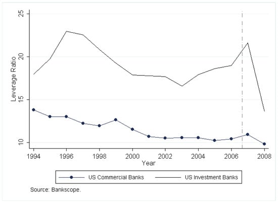
Figure 1.
Average pure balance sheet leverage ratios in USA.
Things change when one moves beyond the simple balance sheet ratio and addresses the core issue of the quality of banking capital. Consider first the case of commercial banks. Figure 2 compares the different measures of leverage: the connected dots show the pure balance sheet ratio (as in Figure 1), the unconnected marks indicate the regulatory tier 1 ratio, and the upper line the prudent leverage ratio introduced in Section 2 (the vertical dashed line on the time axis indicates August 2007). An important result comes immediately to the fore when inspecting Figure 2. The regulatory leverage ratio of commercial banks displayed no significant hike in the pre-crisis period, while their pure leverage ratio, as mentioned above, actually declined over time. Nevertheless, when measuring capital as the prudent tangible common equity, one discovers that the leverage had been increasing markedly starting from the year 2002. Given that the difference between the two solid lines widened over time, an underlying progressive contraction occurred in the tangible common component of total equity (the numerator is the same for both lines). To put it differently, the figure shows that the quality of the capital of the US commercial banking sector had already been declining sharply since the mid 1990s, something that could not be observed when using the traditional measures of leverage. By analyzing further which component of total equity was declining sharply to pin down the effect pictured in Figure 2, I found that almost the entire effect was accounted for by intangible assets.
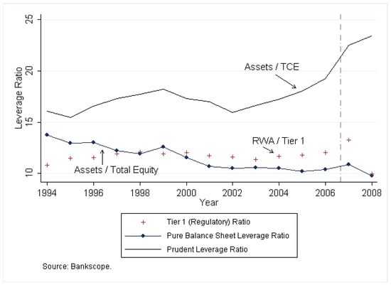
Figure 2.
Average leverage ratios in US commercial banks.
The deterioration in the capital base was weaker for investment banks, as shown in Figure 3. The difference between the two solid lines for the investment banking sector remained almost stable over the sampled period, suggesting that the share of tangible common equity to total equity declined only mildly: no significant capital quality deterioration affected US investment banks.
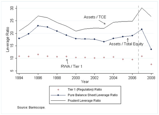
Figure 3.
Average leverage ratios in US investment banks.
A decrease in capital quality before the 2007 crisis characterized approximately half of the countries with regard to commercial banks (especially in the United Kingdom) and almost no country with regard to investment banks (except Switzerland). The decline in capital quality for commercial banks occurred at different intensities across countries. To address this issue, I took the unweighted average of the ratio of TCE to total equity within each country as a proxy for the quality of banking capital. Figure 4 reports the values of this ratio for the first available year on the vertical axis (1994) and for the last year before the crisis on the horizontal axis (2006). The countries in the top-right region are those whose commercial banking sector had on average a higher quality of capital in both years, while countries above (below) the diagonal had a commercial banking sector that experienced a decline (improvement) in banking capital from 1994 to 2006. One can clearly see that, except for Belgium and Finland, all countries were above the diagonal, particularly the Netherlands, Greece, the United States, and the United Kingdom. There are only 15 countries in Figure 4, as the dataset did not include data on commercial banks in the remaining three countries for year 1994.
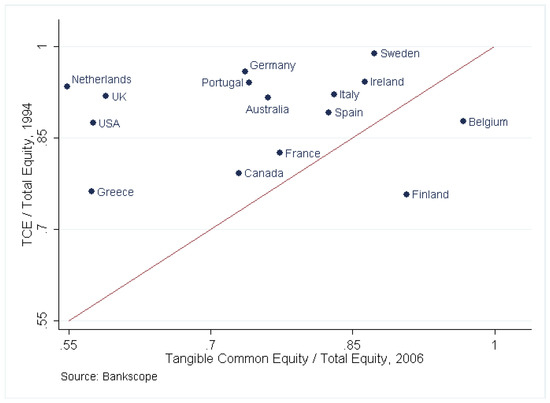
Figure 4.
Cross-country comparison of capital deterioration for commercial banks.
5. More on the Quality of Banking Capital
5.1. Model Specification
The above descriptive evidence suggests that capital quality was declining on average during the period spanned by the dataset, though heterogeneously across banks and countries. In this section, I use multivariate panel regressions to answer two questions:
- Did capital quality decline more for commercial banks than for investment banks, as suggested from the above figures?
- Did capital quality decline equally across big and small banks, or did the balance sheet size play a role?
The research method offered by panel regression analysis was particularly suitable for the analysis presented in this paper. It provides a unified framework that can address multiple unobserved heterogeneities. See [14] for an introduction to panel analysis.
In the following estimated models, capital quality was measured as the percentage deviation of tangible common equity from total equity and computed as the natural log of the TCE/TE ratio. A decrease in the percentage deviation of TCE from TE signaled a decline in the capital quality, as it showed a decline in the tangible component of common contributed capital.
A summary of the statistics is shown in Table 6. One can see that, on average, the quality of banking capital was lower and more volatile for commercial banks (relative to investment banks) and for big banks (relative to small banks).
Table 6.
Average quality of capital: tangible common equity over total equity.
I estimated the different models depending on the hypothesis tested and on the fixed effects and other variables that I controlled for. In the following regressions, the dummy variable took the value of 1 if the bank was a commercial bank. The dummy variable took the value 1 if the bank’s aggregate assets across the years sampled were above 50% of the average aggregate assets computed across banks (alternative threshold values were used in robustness checks).
In all models estimated, I controlled for different accounting standards across banks and years using a dummy variable that took the value 1 after the corresponding bank had adopted the International Financial Reporting Standards. Additionally, fixed effects at the country level controlled for possible national regulatory differences across countries that were not fully reflected in the accounting standard adopted.
5.1.1. Model 1
The first estimated model tested whether the correlations supported the finding that capital declined more significantly for commercial banks than for investment banks. Equation (1) shows the estimated model. A negative and statistically significant coefficient would suggest that commercial banks tended to have a smaller ratio of tangible common equity to total equity. Estimations differed for the combinations of fixed effects at the bank, country, and/or year level.
The regression results are reported in Table 7, which is divided into eight columns, one for each specification considered. As one can see, all coefficients on the dummy variable were negative and statistically significant, mostly at a level of 1%, except for estimation II (positive and significant) and estimation VI (positive but insignificant). The data seemed to support the hypothesis that commercial banks had a lower quality of capital base compared to investment banks.
Table 7.
Regression results for capital quality (model 1).
5.1.2. Model 2
The second estimated model tested whether the correlations supported the finding that capital declined differently between banks with different balance sheet sizes. Equation (2) shows the second estimated model. A negative and statistically significant coefficient would suggest that big banks tended to have a smaller ratio of tangible common equity to total equity. Again, estimations differed for the combinations of fixed effects at the bank, country, and/or year level.
The regression results are reported in Table 8, which is divided into eight columns, one for each estimation considered. As one can see, all coefficients on the dummy variable were negative and statistically significant, mostly at the level of 1%, except for estimation V (positive but insignificant) and estimation VI (negative but insignificant). The data seemed to support the hypothesis that big banks had a lower quality of capital compared to small banks.
Table 8.
Regression results on capital quality (model 2).
5.1.3. Model 3
The third estimated model combines the analysis of both bank specialization and bank asset size. To control for possible endogeneity, two controls were added. The first was a measure of the business cycle, proxied by the output gap computed with an HP filter. The second control was a profitability measure, proxied by the pre-tax bank profits and losses (alternative controls were used for robustness checks).
Equation (3) shows the estimated model. Negative and statistically significant coefficients and had the same meaning as in Equations (2) and (3).
The regression results are reported in Table 8, which shows that the outcomes of the two previous models remained true under this new specification. As one can see, almost all coefficients on the dummy variables and were negative and statistically significant, mostly at the 1% level, except estimations II and V (insignificant) and estimations VI and VIII (one insignificant coefficient).
5.2. Robustness Checks
The results were robust under a variety of alternative settings. I dropped the dummy variable controlling for asset size and divided the sample into two subsamples, depending on the percentile of aggregate assets for each bank across the whole time period. The result that big banks tended to have a worse quality of capital was confirmed by the fact that banks above the average size of aggregate assets still had a negative and significant coefficient on the dummy variable Dcom, while the coefficient became insignificant for small banks.
The result also held when dropping the tails of the distribution of bank asset size, eliminating banks with an aggregate asset size that was either in the first 10 or last 90 percentiles. Additionally, the negative coefficient on Dbig became even larger when excluding investment banks from the sample, confirming that commercial banks had a worse quality of capital (the coefficient was partially insignificant when dropping commercial banks).
I also partitioned the sample into two subsamples for the years before and after the 2007 crisis, but the signs and statistical significance of the estimates remained almost unchanged. The result held even when computing the output gap with the Baxter–King filter instead of the Hodrick–Prescot filter.
The analysis was replicated after clustering the standard errors of Table 7, Table 8 and Table 9 at the bank level. The results showed that the main conclusion regarding the statistical significance of the parameters remained largely unchanged, further supporting the results of the paper.
Table 9.
Regression results on capital quality (model 3).
Caution should be implemented in interpreting Table 7, Table 8 and Table 9, since the signs of the coefficients could be sensitive across the very broad range of specifications considered. To shed light on this point, the Hausman test was used to select between fixed effects and random effects at the bank level. The analysis supported the former specification.
6. Conclusions
The empirical investigation of this paper was justified by the scarce attention paid to commercial banks’ leverage dynamics in interpreting the causes of the 2007 financial crisis. I constructed a panel dataset for the biggest banking groups using balance sheet data pertaining to banks from 20 countries in the period after the full implementation of Basel I (1994–2008).
This paper contributed to the debate by showing that the traditional measures of leverage (risk-weighted assets over tier 1 capital and the book value of assets over total equity) cannot detect an important deterioration in banks’ capital quality that had been ongoing since well before the 2007 crisis. Using the more prudent tangible common equity as a measure of bank capital, this paper compared different leverage measures and investigated the dynamics of capital quality in the period covered by the sample.
The results showed that capital was deteriorating heterogeneously across banks before the crisis, with its quality declining strongly for commercial (and big) banks and mildly for investment (and small) banks. This finding supports the idea that the financial instability that led to the crisis should not be attributed primarily to the investment banking sector, as implied extensively by the existing literature.
Funding
This research received no external funding.
Data Availability Statement
Not applicable.
Conflicts of Interest
The authors declare no conflict of interest.
References
- Adrian, T.; Shin, H.S. Liquidity and financial cycles. Bis Work. Pap. 2008. [Google Scholar] [CrossRef]
- Brunnermeier, M.K. Deciphering the liquidity and credit crunch 2007–2008. J. Econ. Perspect. 2009, 23, 77–100. [Google Scholar] [CrossRef]
- Goodhart, C.A.E. The regulatory response to the financial crisis. In Books; Edward Elgar Publishing: Cheltenham, UK, 2009. [Google Scholar]
- England, B.O. The Role of Macroprudential Policy; Bank of England Discussion Paper; Bank of England: London, UK, 2009. [Google Scholar]
- Brunnermeier, M.; Crockett, A.; Goodhart, C.A.; Persaud, A.; Shin, H.S. The Fundamental Principles of Financial Regulation; International Center for Monetary and Banking Studies (ICMB): Geneva, Switzerland, 2009; Volume 11. [Google Scholar]
- Adrian, T.; Shin, H.S. Liquidity and leverage. J. Financ. Intermediation 2010, 19, 418–437. [Google Scholar] [CrossRef]
- Read, E.; Gill, E. Commercial Banking, 4th ed.; Prentice Hall: Hoboken, NJ, USA, 1989. [Google Scholar]
- Shrieves, R.E.; Dahl, D. The relationship between risk and capital in commercial banks. J. Bank. Financ. 1992, 16, 439–457. [Google Scholar] [CrossRef]
- Rajan, R.G. Why banks have a future: Toward a new theory of commercial banking. J. Appl. Corp. Financ. 1996, 9, 114–128. [Google Scholar] [CrossRef]
- Lu, J.; Hu, X. Novel three-bank model for measuring the systemic importance of commercial banks. Econ. Model. 2014, 43, 238–246. [Google Scholar] [CrossRef]
- Jones, A.M. Panel data methods and applications to health economics. In Palgrave Handbook of Econometrics: Volume 2: Applied Econometrics; Palgrave Macmillan: London, UK, 2009; pp. 557–631. [Google Scholar]
- Dun, Z.; Mitchell, P.; Agosti, M. Estimating Diabrotica virgifera virgifera damage functions with field trial data: Applying an unbalanced nested error component model. J. Appl. Entomol. 2010, 134, 409–419. [Google Scholar] [CrossRef]
- Petersen, M.A. Estimating standard errors in finance panel data sets: Comparing approaches. Rev. Financ. Stud. 2008, 22, 435–480. [Google Scholar] [CrossRef]
- Baltagi, B.H.; Baltagi, B.H. Econometric Analysis of Panel Data; Springer: Berlin/Heidelberg, Germany, 2008; Volume 4. [Google Scholar]
- Sarafidis, V.; Wansbeek, T. Celebrating 40 years of panel data analysis: Past, present and future. J. Econom. 2021, 220, 215–226. [Google Scholar] [CrossRef]
- Wooldridge, J.M. Distribution-free estimation of some nonlinear panel data models. J. Econom. 1999, 90, 77–97. [Google Scholar] [CrossRef]
- Arellano, M.; Bonhomme, S. Nonlinear panel data analysis. Annu. Rev. Econ. 2011, 3, 395–424. [Google Scholar] [CrossRef]
- Nuno, G.; Thomas, C. Bank leverage cycles. Am. Econ. J. Macroecon. 2017, 9, 32–72. [Google Scholar] [CrossRef]
- Dell’Ariccia, G.; Laeven, L.; Suarez, G.A. Bank leverage and monetary policy’s risk-taking channel: Evidence from the United States. J. Financ. 2017, 72, 613–654. [Google Scholar] [CrossRef]
- Valencia, F. Monetary policy, bank leverage, and financial stability. J. Econ. Dyn. Control 2014, 47, 20–38. [Google Scholar] [CrossRef]
- Christensen, I.; Meh, C.; Moran, K. Bank leverage regulation and macroeconomic dynamic. CIRANO-Sci. Publ. 2011s-76 2011. [Google Scholar] [CrossRef]
- Dell’Ariccia, G.; Laeven, L.; Marquez, R. Real interest rates, leverage, and bank risk-taking. J. Econ. Theory 2014, 149, 65–99. [Google Scholar] [CrossRef]
- Kalemli-Ozcan, S.; Sorensen, B.; Yesiltas, S. Leverage across firms, banks, and countries. J. Int. Econ. 2012, 88, 284–298. [Google Scholar] [CrossRef]
- Tarullo, D.K. Banking on Basel: The Future of International Financial Regulation; Peterson Institute: Washington, DC, USA, 2008. [Google Scholar]
- BIS. Strengthening the resilience of the banking section. In Bank of International Settlemenr, Consultative Document; BIS: Basel, Switzerland, 2009. [Google Scholar]
- Elliott, D.J. Interpreting the Bank Stress Tests; Initiative on Business and Public Policy at Brookings. 2009. Available online: www.brookings.edu/research/interpreting-the-bank-stress-tests (accessed on 20 February 2023).
- Berger, A.N.; Herring, R.J.; Szegö, G.P. The role of capital in financial institutions. J. Bank. Financ. 1995, 19, 393–430. [Google Scholar] [CrossRef]
Disclaimer/Publisher’s Note: The statements, opinions and data contained in all publications are solely those of the individual author(s) and contributor(s) and not of MDPI and/or the editor(s). MDPI and/or the editor(s) disclaim responsibility for any injury to people or property resulting from any ideas, methods, instructions or products referred to in the content. |
© 2023 by the author. Licensee MDPI, Basel, Switzerland. This article is an open access article distributed under the terms and conditions of the Creative Commons Attribution (CC BY) license (https://creativecommons.org/licenses/by/4.0/).