Article

Approximate Roots and Properties of Differential Equations for Degenerate q-Special Polynomials

by
Jung-Yoog Kang
1 and
Cheon-Seoung Ryoo
2,*
1
Department of Mathematics Education, Silla University, Busan 46958, Republic of Korea
2
Department of Mathematics, Hannam University, Daejeon 34430, Republic of Korea
*
Author to whom correspondence should be addressed.
Mathematics 2023, 11(13), 2803; https://doi.org/10.3390/math11132803
Submission received: 15 April 2023 / Revised: 5 June 2023 / Accepted: 20 June 2023 / Published: 21 June 2023
(This article belongs to the Special Issue Q-differential/Difference Equations and Related Applications)

Abstract

:
In this paper, we generate new degenerate quantum Euler polynomials (DQE polynomials), which are related to both degenerate Euler polynomials and q-Euler polynomials. We obtain several ( q , h ) -differential equations for DQE polynomials and find some relations of q-differential and h-differential equations. By varying the values of q , η , and h, we observe the values of DQE numbers and approximate roots of DQE polynomials to obtain some properties and conjectures.
MSC:
34A25; 33F05; 11B68; 65H04

1. Basic Concepts and Introduction

Before clarifying the objectives of this paper, we first introduce the necessary basic concepts. We identify several definitions and properties and present the goals of this paper based on them.
Let η , q R with q 1 . The quantum number, q-number, discovered by Jackson is
[ η ] q = 1 q η 1 q ,
and we note that lim q 1 [ η ] q = η . In particular, for k Z , [ k ] q is called q-integer; see [1,2,3,4].
Many mathematicians in various fields have worked on the introduction of q-numbers, such as q-discrete distribution, q-differential equations, q-series, q-calculus, and so on; see [5,6,7,8].
The following equation,
m r q = [ m ] q ! [ m r ] q ! [ r ] q ! ,
is the q-Gaussian binomial coefficient where m and r are non-negative integers; see [4,5]. For r = 0 , the value of q-Gaussian binomial coefficients is 1 since the numerator and the denominator are both empty products. One notes that [ η ] q ! = [ η ] q [ η 1 ] q [ 2 ] q [ 1 ] q and [ 0 ] q ! = 1 .
In [9], a two-parameter time scale T q , h was introduced as follows:
T q , h : = { q η ψ + [ η ] q h | ψ R , η Z , h , q R + , q 1 } { h 1 q } .
Definition 1 
([9,10]). Let f : T q , h R be any function. Then, the delta ( q , h ) -derivative of f D q , h ( f ) is defined by
D q , h f ( ψ ) : = f ( q ψ + h ) f ( ψ ) ( q 1 ) ψ + h .
From the above definition, we can see several properties as follows:
(i)
For ψ T q , h , D q , h f ( ψ ) = 0 if and only if f ( ψ ) is a constant;
(ii)
D q , h f ( ψ ) = D q , h g ( ψ ) for all ψ T q , h if and only if f ( ψ ) = g ( ψ ) + c with some constant c;
(iii)
For ψ T q , h , D q , h f ( ψ ) = c 1 if and only if f ( ψ ) = c 1 ψ + c 2 , where c 1 and c 2 are constant.
In Definition 1, we can see that D q , h ( f ) , the delta ( q , h ) -derivative of f reduces to D q ( f ) , the q-derivative of f for h 0 and reduces to D h ( f ) , the h-derivative of f for q 1 .
In addition, we can find the product rule and quotient rule for the delta ( q , h ) -derivative.
Theorem 1 
([9,10]). Let f , g be arbitrary functions.
( i ) Product   rule D q , h ( f ( ψ ) g ( ψ ) ) = g ( q ψ + h ) D q , h f ( ψ ) + f ( ψ ) D q , h g ( ψ ) = f ( q ψ + h ) D q , h g ( ψ ) + g ( ψ ) D q , h f ( ψ ) . ( ii ) Quotient   rule D q , h f ( ψ ) g ( ψ ) = g ( ψ ) D q , h f ( ψ ) f ( ψ ) D q , h g ( ψ ) g ( ψ ) g ( q ψ + h ) = g ( q ψ + h ) D q , h f ( ψ ) f ( q ψ + h ) D q , h g ( ψ ) g ( ψ ) g ( q ψ + h ) .
Definition 2 
([10,11]). The generalized quantum binomial ( ψ ψ 0 ) q , h η is defined by
( ψ ψ 0 ) q , h η : = 1 , if η = 0 , i = 1 η ψ ( q i 1 ψ 0 + [ i 1 ] q h ) , if η > 0 ,
where ψ 0 R .
The generalized quantum binomial reduces to q-binomial ( ψ ψ 0 ) q η as h 0 and to h-binomial ( ψ ψ 0 ) h η when q 1 . Also, we note lim ( q , h ) ( 1 , 0 ) ( ψ ψ 0 ) q , h η = ( ψ ψ 0 ) η .
Definition 3 
([10]). The generalized quantum exponential function exp q , h ( α ψ ) is defined as
exp q , h ( α ψ ) : = i = 0 α i ( ψ 0 ) q , h i [ i ] q ! ,
where α is an arbitrary nonzero constant.
Clearly, we note exp q , h ( 0 ) = 1 . As h 0 and α = 1 , the generalized quantum exponential function exp q , h ( α ψ ) becomes the so-called q-exponential function e q ( ψ ) ; see [4,5]. Also, as q 1 and α = 1 , the generalized quantum exponential function exp q , h ( α ψ ) reduces to the so-called h-exponential function e h ( ψ ) = ( 1 + h ) ψ h ; see [4].
Based on the above concepts, many mathematicians have studied q-special functions, q-differential equations, q-calculus, and so on; see [12,13,14,15,16]. For example, Duran, Acikgoz and Araci [16] considered different trigonometric functions and hyperbolic functions related to quantum numbers and looked for properties related to them. Mathematicians also discovered various theorems about basic concepts related to h-numbers. Benaoum [11] obtained Newton’s binomial formula in terms of ( q , h ) , and Cermak and Nechvatal [9] created a ( q , h ) version of fractional calculus. In 2011, Rahmat [17] studied the ( q , h ) -Laplace transform. Silindir and Yantir [10] studied the quantum generalization of Taylor’s formula and the q-binomial coefficient in 2019; their work motivated the research reported in this paper. Mathematicians who study polynomials have already defined and characterized degenerate Euler polynomials. They also studied the definition and properties of Euler polynomials when combined with quantum numbers.
The main purpose of this paper is to construct degenerate quantum Euler polynomials (DQE polynomials) using properties of q-numbers and the ( q , h ) -derivative. The topic of this paper is a field of mathematics that can be expanded into subareas such as series methods or generalizations of existing series. Its results can also be applied in interdisciplinary areas such as nonlinear physics, as well as for solutions to nonlinear differential equations providing instrumental defects such as kinks, vortices, etc. The diagram below shows the relationship of Euler, q-Euler, and degenerate Euler polynomials to the degenerate quantum Euler polynomials (DQE polynomials) that we define here.
Mathematics 11 02803 i001
Definition 4 
([14,18]). q-Euler numbers and polynomials are defined as:
η = 0 E η , q τ η [ η ] q ! = 2 e q ( τ ) + 1 , η = 0 E η , q ( ψ ) τ η [ η ] q ! = 2 e q ( τ ) + 1 e q ( τ ψ ) .
Definition 5 
([19,20]). Degenerate Euler numbers and polynomials are defined as:
η = 0 E η ( h ) τ η η ! = 2 e h ( 1 : τ ) + 1 , η = 0 E η ( ψ : h ) τ η η ! = 2 e h ( 1 : τ ) + 1 e h ( ψ : τ ) .
The structure of this paper is as follows. In Section 2, we define DQE numbers and polynomials. We find several properties of these polynomials by using q-numbers and ( q , h ) -derivatives. In addition, we construct several higher-order differential equations whose solutions are DQE polynomials. Section 3 shows the structure of approximate roots of DQE polynomials, which are solutions of the higher-order differential equations obtained in Section 2. By observing various structures of these approximate roots, we can make several conjectures.

2. ( q , h ) -Differential Equations That are Related to DQE Polynomials

In this section, we define a degenerate q-exponential function and DQE numbers and polynomials. We find several ( q , h ) -differential equations that are related to DQE polynomials by the ( q , h ) -derivative. We also discuss how these DQE polynomials relate to both q-Euler polynomials and degenerate Euler polynomials. We introduce the following degenerate quantum exponential function:
e q , h ( ψ : τ ) : = η = 0 ( ψ ) q , h η τ η η ! = η = 0 k = 0 η ψ [ k 1 ] q h τ η η ! .
For example, substituting ψ = 1 in the above equation, we have
e q , h ( 1 : τ ) = η = 0 ( 1 ) q , h η τ η η ! ,
where ( 1 ) q , h n = 1 ( 1 h ) ( 1 [ n 1 ] q h ) .
Definition 6. 
Let | q | < 1 and let h be a non-negative integer. Then, we define the DQE polynomials E η , q ( ψ : h ) as:
η = 0 E η , q ( ψ : h ) τ η [ η ] q ! = 2 e q , h ( 1 : τ ) + 1 e q , h ( ψ : τ ) .
When ψ = 0 , we can note that
η = 0 E η , q ( h ) τ η [ η ] q ! = 2 e q , h ( 1 : τ ) + 1 .
We denote E η , q ( h ) as the DQE numbers. From Definition 6, we can see several relationships between Euler polynomials. Setting h 0 in Definition 6, we can find the q-Euler numbers E η , q and polynomials E η , q ( ψ ) as
η = 0 E η , q τ η [ η ] q ! = 2 e q ( τ ) + 1 , η = 0 E η , q ( ψ ) τ η [ η ] q ! = 2 e q ( τ ) + 1 e q ( τ ψ ) .
Let h 0 and q 1 in Definition 6. Then, we have the Euler numbers E η and polynomials E η ( ψ ) as
η = 0 E η τ η η ! = 2 e τ + 1 , η = 0 E η ( ψ ) τ η η ! = 2 e τ + 1 e τ ψ .
In addition, for q 1 in Definition 6, we can see the degenerate Euler numbers E η ( h ) and polynomials E η ( ψ : h ) as follows:
η = 0 E η ( h ) τ η η ! = 2 e h ( 1 : τ ) + 1 , η = 0 E η ( ψ : h ) τ η η ! = 2 e h ( 1 : τ ) + 1 e h ( ψ : τ ) ,
where E η ( h ) = E η ( 0 : h ) .
Theorem 2. 
Let | q | < 1 and h N . Then, we have
D q , h E η , q ( ψ : h ) = [ η ] q E η 1 , q ( ψ : h ) .
Proof. 
From the generating function of the DQE polynomials, we can find
η = 0 E η , q ( ψ : h ) τ η [ η ] q ! = η = 0 E η , q ( h ) τ η [ η ] q ! η = 0 ( ψ ) q , h η τ η [ η ] q ! = η = 0 k = 0 η η k q ( ψ ) q , h η k E k , q ( h ) τ η [ η ] q ! .
Applying the coefficient comparison method to the above equation, we find a relation of DQE numbers and polynomials such as
E η , q ( ψ : h ) = k = 0 η η k q ( ψ ) q , h η k E k , q ( h ) .
Using the ( q , h ) -derivative in Equation (1), we can obtain the following equation:
D q , h E η , q ( ψ : h ) = k = 0 η η k q [ η k ] q ( ψ ) q , h η k 1 E k , q ( h ) .
Considering Equation (1) and the above equation together, we have the required result. □
Corollary 1. 
Let k be a non-negative integer. From Theorem 2, one holds
E η k , q ( ψ : h ) = [ η k ] q ! [ η ] q ! D q , h ( k ) E η , q ( ψ : h ) .
Corollary 2. 
From Theorem 2, the following holds:
(i) Setting q 1 in Theorem 2, we have
D h E η ( ψ : h ) = η E η 1 ( ψ : h ) , E η k ( ψ : h ) = ( η k ) ! η ! D h ( k ) E η ( ψ : h ) ,
where D h is the h-derivative and E η ( ψ : h ) is the degenerate Euler polynomial.
(ii) Putting h 0 in Theorem 2, we have
D q E η , q ( ψ ) = [ η ] q E η 1 , q ( ψ ) , E η k , q ( ψ ) = [ η k ] q ! [ η ] q ! D q ( k ) E η , q ( ψ ) ,
where D q is the q-derivative and E η , q ( ψ ) is the q-Euler polynomial.
Theorem 3. 
The DQE polynomials represent a solution of the ( q , h ) -differential equation of higher order shown below:
( 1 ) q , h η [ η ] q ! D q , h ( η ) E η , q ( ψ : h ) + ( 1 ) q , h η 1 [ η 1 ] q ! D q , h ( η 1 ) E η , q ( ψ : h ) + ( 1 ) q , h η 2 [ η 2 ] q ! D q , h ( η 2 ) E η , q ( ψ : h ) + + ( 1 ) q , h 2 [ 2 ] q ! D q , h ( 2 ) E η , q ( ψ : h ) + ( 1 ) q , h 1 D q , h ( 1 ) E η , q ( ψ : h ) + 2 E η , q ( ψ : h ) 2 ( ψ ) q , h η = 0 .
Proof. 
Consider e q , h ( 1 : τ ) 1 in the generating function of the DQE polynomials. Then, we have
η = 0 E η , q ( ψ : h ) τ η [ η ] q , h ! e q , h ( 1 : τ ) + 1 = 2 e q , h ( ψ : τ ) .
The left-hand side of Equation (2) is transformed as
η = 0 E η , q ( ψ : h ) τ η [ η ] q ! e q , h ( 1 : τ ) + 1 = η = 0 k = 0 η n k q ( 1 ) q , h k E η k , q , h ( ψ ) + E η , q ( ψ : h ) τ η [ η ] q ! .
The right-hand side of Equation (2) is changed as
2 e q , h ( ψ : τ ) = 2 η = 0 ψ q , h η t η [ η ] q ! .
From the above equations, we can obtain
k = 0 η η k q ( 1 ) q , h k E η k , q ( ψ : h ) + E η , q ( ψ : h ) = 2 ( ψ ) q , h η .
Considering both Corollary 2 and Equation (3), we have
k = 0 η ( 1 ) q , h k [ k ] q ! D q , h ( k ) E η , q ( ψ : h ) + E η , q ( ψ : h ) 2 ( ψ ) q , h η = 0 ,
which is the desired result. □
Corollary 3. 
Setting q 1 in Theorem 3, it holds that:
( 1 ) h η η ! D h ( η ) E η ( ψ : h ) + ( 1 ) h η 1 ( η 1 ) ! D h ( η 1 ) E η ( ψ : h ) + ( 1 ) h η 2 ( η 1 ) ! D h ( η 2 ) E η ( ψ : h ) + + ( 1 ) h 2 2 ! D h ( 2 ) E η ( ψ : h ) + ( 1 ) h D h ( 1 ) E η ( ψ : h ) + 2 E η ( ψ : h ) 2 ( ψ ) h η = 0 ,
where D h is the h-derivative and E η ( ψ : h ) is the degenerate Euler polynomial.
Corollary 4. 
Let h 0 in Theorem 3. Then, it holds that:
1 [ η ] q ! D q ( η ) E η , q ( ψ ) + 1 [ η 1 ] q ! D q ( η 1 ) E η , q ( ψ ) + 1 [ η 2 ] q ! D q ( η 2 ) E η , q ( ψ ) + + 1 [ 2 ] q ! D q ( 2 ) E η , q ( ψ ) + D q ( 1 ) E η , q ( ψ ) + 2 E η , q ( ψ ) 2 ψ η = 0 ,
where D q is the q-derivative and E η , q ( ψ ) is the q-Euler polynomial.
Theorem 4. 
DQE polynomials are the solutions to the ( q , h ) -differential equation of higher order as
E η , q ( 1 : h ) + E η , q ( h ) [ η ] q ! D q , h ( η ) E η , q ( ψ : h ) + E η 1 , q ( 1 : h ) + E η 1 , q ( h ) [ η 1 ] q ! D q , h ( η 1 ) E η , q ( ψ : h ) + + E 2 , q ( 1 : h ) + E 2 , q ( h ) [ 2 ] q ! D q , h ( 2 ) E η , q ( ψ : h ) + ( E 1 , q ( 1 : h ) + E 1 , q ( h ) ) D q , h ( 1 ) E η , q ( ψ : h ) + E 0 , q ( 1 : h ) + E 0 , q ( h ) 2 E η , q ( ψ : h ) = 0 .
Proof. 
From Definition 6, we have
η = 0 E η , q ( ψ : h ) τ η [ η ] q ! = 2 e q , h ( 1 : τ ) + 1 e q , h ( ψ : τ ) = 1 2 2 e q , h ( 1 : τ ) + 1 e q , h ( 1 : τ ) + 2 e q , h ( 1 : τ ) + 1 2 e q , h ( 1 : τ ) + 1 e q , h ( ψ : τ ) .
Using the generating function of DQE polynomials, we find the following relation:
2 η = 0 E η , q ( ψ : h ) τ η [ η ] q ! = η = 0 k = 0 η η k q E k , q , h ( 1 ) + E k , q , h E η k , q , h ( ψ ) τ η [ η ] q ! .
Comparing the coefficients of both sides, we obtain
k = 0 η η k q E k , q ( 1 : h ) + E k , q ( h ) E η k , q ( ψ : h ) 2 E η , q ( ψ : h ) = 0 .
Replacing D q , h ( k ) E η , q ( ψ : h ) for E η k , q ( ψ : h ) in Equation (4), we derive
k = 0 η E k , q ( 1 : h ) + E k , q ( h ) [ k ] q ! D q , h ( k ) E η , q ( ψ : h ) 2 E η , q ( ψ : h ) = 0 .
The equation above completes the proof of Theorem 4. □
Corollary 5. 
Setting h 0 in Theorem 4, it holds that:
E η , q ( 1 ) + E η , q [ η ] q ! D q ( η ) E η , q ( ψ ) + E η 1 , q ( 1 ) + E η 1 , q [ η 1 ] q ! D q , ψ ( η 1 ) E η , q ( ψ ) + + E 2 , q ( 1 ) + E 2 , q [ 2 ] q ! D q ( 2 ) E η , q ( ψ ) + ( E 1 , q ( 1 ) + E 1 , q ) D q ( 1 ) E η , q ( ψ ) + E 0 , q , ( 1 ) + E 0 , q 2 E η , q ( ψ ) = 0 ,
where D q is the q-derivative and E η , q ( ψ ) is the q-Euler polynomial.
Corollary 6. 
Putting q 1 in Theorem 4, the following holds:
E η ( 1 : h ) + E η ( h ) η ! D h ( η ) E η ( ψ : h ) + E η 1 ( 1 : h ) + E η 1 ( h ) ( η 1 ) ! D h ( η 1 ) E η ( ψ : h ) + + E 2 ( 1 : h ) + E 2 ( h ) 2 ! D h ( 2 ) E η ( ψ : h ) + ( E 1 ( 1 : h ) + E 1 ( h ) ) D h ( 1 ) E η ( ψ : h ) + E 0 ( 1 : h ) + E 0 ( h ) 2 E η ( ψ : h ) = 0 ,
where D h is the h-derivative and E η ( ψ : h ) is the degenerate Euler polynomial.
From a property of e q , h ( ψ : τ ) , we note a relation
e q , h ( q ψ : τ ) = η = 0 q ψ ( q ψ h ) ( q ψ [ 2 ] q h ) ( q ψ [ 3 ] q h ) ( q ψ [ η 1 ] q h ) τ η [ η ] q ! = e q , q 1 h ( ψ : q τ ) .
Theorem 5. 
The following higher-order differential equation has DQE polynomials as the solution:
q η E η , q ( 1 : q 1 h ) + E η , q ( q 1 h ) [ η ] q ! D q , h ( η ) E η , q ( ψ : h ) + q η 1 E η 1 , q ( 1 : q 1 h ) + E η 1 , q ( q 1 h ) [ η 1 ] q ! D q , h ( η 1 ) E η , q ( ψ : h ) + + q 2 E 2 , q ( 1 : q 1 h ) + E 2 , q ( q 1 h ) [ 2 ] q ! D q , h ( 2 ) E η , q ( ψ : h ) + q ( E 1 , q ( 1 : q 1 h ) + E 1 , q ( q 1 h ) ) D q , h ( 1 ) E η , q ( ψ : h ) + E 0 , q ( 1 : q 1 h ) + E 0 , q ( q 1 h ) 2 E η , q ( ψ : h ) = 0 .
Proof. 
Consider Equation (5) in the generating function of the DQE polynomials. Then, we find
η = 0 E η , q ( q ψ : h ) τ η [ η ] q ! = 2 e q , h ( 1 : τ ) + 1 e q , h ( q ψ : τ ) = 1 2 2 e q , q 1 h ( 1 : q τ ) + 1 e q , q 1 h ( 1 : q τ ) + 2 e q , q 1 h ( 1 : q τ ) + 1 × 2 e q , h ( 1 : τ ) + 1 e q , h ( q ψ : τ ) .
From E n , q ( ψ : h ) , we have the relation
2 η = 0 E η , q ( q ψ : h ) τ η [ η ] q ! = η = 0 k = 0 η η k q q k E k , q ( 1 : q 1 h ) + E k , q ( q 1 h ) E η k , q ( q ψ : h ) τ η [ η ] q ! .
From the above equation, we find
k = 0 η η k q q k E k , q ( 1 : q 1 h ) + E k , q ( q 1 h ) E η k , q ( q ψ : h ) 2 E η , q ( q ψ : h ) = 0 .
Substituting q ψ for ψ in Corollary 2, we note that
E η k , q ( q ψ : h ) = [ η k ] q ! [ η ] q ! D q , h ( k ) E η , q ( q ψ : h ) .
Applying the above equation in Equation (6), we have
k = 0 η q k E k , q ( 1 : q 1 h ) + E k , q ( q 1 h ) [ k ] q ! D q , h ( k ) E η , q ( q ψ : h ) 2 E η , q ( q ψ : h ) = 0 ,
which gives the required result. □
Corollary 7. 
Setting h 0 in Theorem 5, it holds that:
q η E η , q ( 1 ) + E η , q [ η ] q ! D q ( η ) E η , q ( ψ ) + q η 1 E η 1 , q ( 1 ) + E η 1 , q [ η 1 ] q ! D q ( η 1 ) E η , q ( ψ ) + + q 2 E 2 , q ( 1 ) + E 2 , q [ 2 ] q ! D q ( 2 ) E η , q ( ψ ) + q ( E 1 , q ( 1 ) + E 1 , q ) D q ( 1 ) E η , q ( ψ ) + E 0 , q ( 1 ) + E 0 , q 2 E η , q ( ψ ) = 0 ,
where D q is the q-derivative and E η , q ( ψ ) is the q-Euler polynomial.

3. Properties for Approximate Roots of DQE Polynomials

In this section, we use Mathematica to show the structures and shapes of approximate roots of DQE polynomials. These DQE polynomials share several properties with both degenerate Euler polynomials and q-Euler polynomials. Here, the purpose of changing the q-number is to explore the properties of q-Euler polynomials, while the reason for changing the value of h is to explore the properties of degenerate Euler polynomials.
Let e q , h ( 1 : τ ) 1 . From the generating function of DQE numbers, we have
η = 0 E η , q ( h ) τ η [ η ] q ! η = 0 ( 1 ) q , h η τ η [ η ] q ! + 1 = 2 .
Using the Cauchy product in the above equation, we obtain
η = 0 k = 0 η η k q ( 1 ) q , h k E η k , q ( h ) + E η , q ( h ) τ η [ η ] q ! = 2 .
Therefore, we derive
k = 0 η η k q ( 1 ) q , h k E η k , q ( h ) + E η , q ( h ) = 2 , if η = 0 , 0 , otherwise .
From the above equation, we show several DQE numbers E η , q , h as follows:
E 0 , q ( h ) = 1 , E 1 , q ( h ) = 1 2 , E 2 , q ( h ) = 1 4 ( 1 + 2 h q ) , E 3 , q ( h ) = 1 8 ( 4 h 2 ( 1 + q ) + 4 h ( 2 + q ) + ( 1 + q ) ( 1 + ( 3 + q ) q ) ) , E 4 , q ( h ) = 1 16 ( 8 h 3 ( 1 + q ) ( 1 + q + q 2 ) ( 1 + q ) ( 1 + q ) ( 1 + ( 4 + q ) q ) ( 1 + q + q 2 ) + 4 h 2 ( 1 + q ) ( 5 + q ( 2 + ( 2 + q ) q ) ) + 2 h ( 11 + q ( 6 + q q 2 ( 3 + q ( 2 + q ) ) ) ) ) , .
Figure 1 shows the values of E η , q , h obtained by varying the values of q, η , and h. Non-negative integers on the x-axis in Figure 1 represent the value of η , with the 0 mark on the x-axis corresponding to E 0 , q , h , the 1 mark indicating E 1 , q , h , and so on. The lines represent variations of the approximate values for DQE numbers. The approximate values of ( 0.1 , h ) -Euler numbers in Figure 1a are the blue dots, yellow squares, green rhombuses, and red triangles, respectively, for η = 0 , 2 , 4 , 6 . Here, we can think of the blue dots as approximate values of q-Euler numbers. In Figure 1b, the blue dots, yellow squares, green rhombuses, and red triangles are the approximate values of ( q , 2 ) -Euler numbers in the respective cases q = 0.3 , 0.5 , 0.7 , 0.9 . The red triangles can be thought of as approximate values of h-Euler numbers.
We next consider the approximate roots of DQE polynomials. In order to identify some of these approximate roots and their properties, we need the exact shapes of the polynomials. Several DQE polynomials E η , q ( ψ : h ) are shown in the following:
E 0 , q ( ψ : h ) = 1 , E 1 , q ( ψ : h ) = 1 2 + ψ , E 2 , q ( ψ : h ) = 1 4 ( 1 + 2 h + q 2 ( 1 + 2 h + q ) ψ + 4 ψ 2 ) , E 3 , q ( ψ : h ) = 1 8 ( ( 1 + q ) ( 1 + 4 h 2 + 4 h ( 1 + q ) + ( 3 + q ) q ) ) + 1 4 ( 1 + q 3 + 4 h 2 ( 1 + q ) + 4 h ( 1 + q + q 2 ) ) ψ 1 2 ( 1 + q + q 2 + 2 h ( 2 + q ) ) ψ 2 + ψ 3 , .
Based on the DQE polynomials obtained above, we hope to find out about the various behaviors of their approximate roots according to the changes in the values of q and h. We will restrict the value of q to less than 1, since DQE polynomials become degenerate Euler polynomials when q approaches 1 Also, DQE polynomials become q-Euler polynomials when h goes to 0, so the value of h has to exclude 0. According to the above condition, we can check the structures of approximate roots of DQE polynomials. Consider the case when the value of h is changed and but the value of q is fixed.
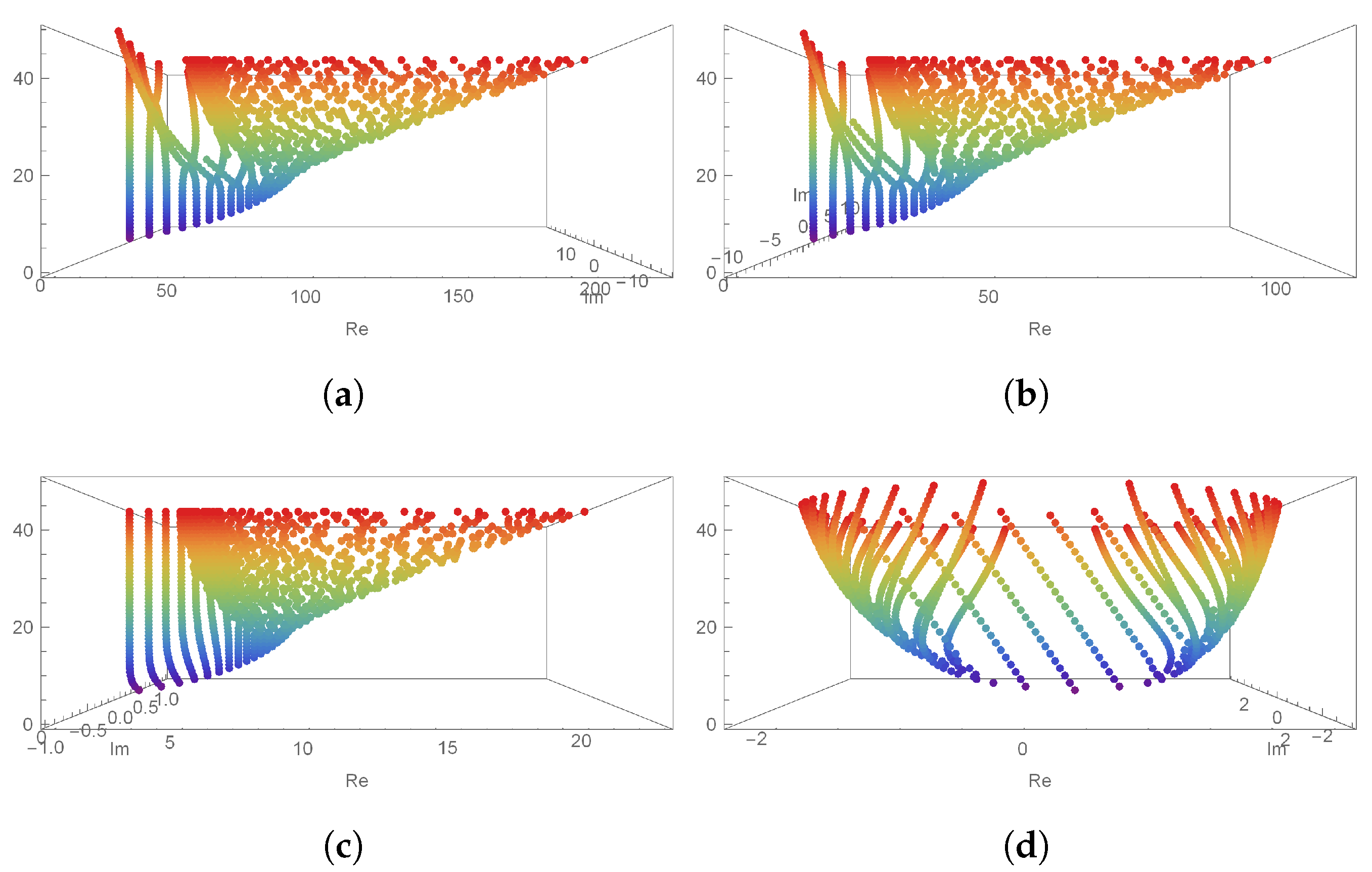
Let us fix 0 η 50 and q = 0.9 . Then, Figure 2 illustrates the structures of the approximate roots of DQE polynomials obtained by varying h. The condition of the top-left panel Figure 2a shows the case where h = 10 ; the condition of the top-right Figure 2b is shown when h = 5 ; the condition of the bottom-left Figure 2c is shown when h = 1 ; and the condition of the bottom-right Figure 2d is shown when h = 0 . From Figure 2d, it can be seen that, when the value of h becomes 0, the shape of the approximate roots reduces to the approximate roots of q-Euler polynomials. The blue dots are the positions of the approximate roots that appear when the value of n is small, and the red dots are the positions of the approximate roots that appear when n = 50 in Figure 2, Figure 3, Figure 4 and Figure 5.
Looking at Figure 2 from above gives the features shown in Figure 3. There, we can see an interesting phenomenon: Figure 3 shows the change in h with q = 0.9 fixed for 0 n 50 . For h = 10 , it seems that all values of real numbers are approximate roots in Figure 3a. In Figure 3b with h = 1 , it can be seen that the approximate roots all have values of real numbers. In Figure 3c, where h = 0 , we see that the shapes of the approximate roots have symmetric properties.
Based on Figure 3, we can see real values shown in Table 1, which shows approximate values of real numbers that appear when h is changed.
Table 1 shows that the numbers of approximate real roots match the value of η when h is 1. When h is 1, the numbers of approximated real roots are also equal to the value of n. However, when h is 0, we can see that the approximated roots come out with both real and imaginary values. Considering Figure 2 and Figure 3, and Table 1, we can make the following conjecture:
Conjecture 1. 
Let us fix q = 0.9 . If 0 η 50 , h = 1 , then all values of approximate roots for DQE polynomials will be found on the real axis.
Figure 4 shows the shapes that appear when q is fixed at q = 0.1 . The conditions of panels (a), (b), and (c) in Figure 4 are as follows:
(a)
E η , 0.1 ( ψ : 10 ) for 0 η 50 ,
(b)
E η , 0.1 ( ψ : 5 ) for 0 η 50 ,
(c)
E η , 0.1 ( ψ : 1 ) for 0 η 50 .
In Figure 4, the blue dots correspond to η = 0 , and the red dots indicate η = 50 . In (a), (b), and (c) of Figure 4, it can be seen that the approximate roots continue to accumulate even if η increases and the value of h changes at one position.
Table 2 shows the approximate roots of one pillar location in Figure 4; we can see that the positions of approximate roots stacked are close to 0. Based on Figure 4 and Table 2, we can make the following conjecture:
Conjecture 2. 
One of the approximate roots of the DQE polynomial has a value close to zero under the conditions q = 0.1 , 0 η 50 , and 1 h 10 .
Next, we explore further properties of DQE polynomials by varying the q-number, given the conditions h = 1 and 0 η 50 . Figure 5 shows a view from above of the 3D shape that appears when the q-number is changed under these constraints. The blue dots represent the low values of n; the red dots indicate where n = 50 . In Figure 5, the q value of the shape on the left is 0.0001 , the q value in the middle is 0.001 , and the q value on the right is 0.5 . Figure 5 shows that the position of the red dots changes according to the value of q and, based on this, we can make the following conjecture:
Conjecture 3. 
Let us fix h = 1 . Then, all values of approximate roots for higher-order DQE polynomials will appear on the real axis as the q-number approaches 0.

4. Conclusions

In this paper, we have introduced DQE polynomials and found higher-order differential equations related to these polynomials. By separately varying the q-number and the h-number of these DQE polynomials, we have shown some properties of their approximate roots and the structure of those roots. We have proposed several further conjectures on questions of interest which we hope will lead to new theorems and properties. This result can be applied to nonlinear physics or problems of finding solutions to nonlinear differential equations. Furthermore, we think the study of quantum polynomials with two variables is an interesting topic.

Author Contributions

Methodology, J.-Y.K. and C.-S.R.; writing—original draft, J.-Y.K.; visualization, C.-S.R. All authors have read and agreed to the published version of the manuscript.

Funding

This research received no external funding.

Data Availability Statement

Not applicable.

Conflicts of Interest

The authors declare no conflict of interest.

References

  1. Jackson, H.F. q-Difference equations. Am. J. Math. 1910, 32, 305–314. [Google Scholar] [CrossRef]
  2. Jackson, H.F. On q-functions and a certain difference operator. Trans. R. Soc. Edinb. 1909, 46, 253–281. [Google Scholar] [CrossRef]
  3. Cao, J.; Zhou, H.-L.; Arjika, S. Generalized q-difference equations for (q,c)-hypergeometric polynomials and some applications. Ramanujan J. 2023, 60, 1033–1067. [Google Scholar] [CrossRef]
  4. Kac, V.; Cheung, P. Quantum Calculus; Part of the Universitext book Series (UTX); Springer: Basel, Switzerland, 2002; ISBN 978-0-387-95341-0. [Google Scholar]
  5. Bangerezako, G. Variational q–calculus. J. Math. Anal. Appl. 2004, 289, 650–665. [Google Scholar] [CrossRef] [Green Version]
  6. Carmichael, R.D. The general theory of linear q-difference equations. Am. J. Math 1912, 34, 147–168. [Google Scholar] [CrossRef]
  7. Duran, U.; Acikgoz, M.; Araci, S. A Study on Some New Results Arising from (p,q)-Calculus. Preprints 2018. [Google Scholar] [CrossRef] [Green Version]
  8. Mason, T.E. On properties of the solution of linear q-difference equations with entire function coefficients. Am. J. Math. 1915, 37, 439–444. [Google Scholar] [CrossRef]
  9. Cermak, J.; Nechvatal, L. On (q,h)-analogue of fractional calculus. J. Nonlinear Math. Phys. 2010, 17, 51–68. [Google Scholar] [CrossRef] [Green Version]
  10. Silindir, B.; Yantir, A. Generalized quantum exponential function and its applications. Filomat 2019, 33, 4907–4922. [Google Scholar] [CrossRef]
  11. Benaoum, H.B. (q,h)-analogue of Newton’s binomial Formula. J. Phys. A Math. Gen. 1999, 32, 2037–2040. [Google Scholar] [CrossRef]
  12. Endre, S.; David, M. An Introduction to Numerical Analysis; Cambridge University Press: Cambridge, UK, 2003; ISBN 0-521-00794-1. [Google Scholar]
  13. Konvalina, J. A unified interpretation of the binomial coefficients, the Stirling numbers, and the Gaussian coefficients. Am. Math. Mon. 2000, 107, 901–910. [Google Scholar] [CrossRef]
  14. Luo, Q.M.; Srivastava, H.M. q-extension of some relationships between the Bernoulli and Euler polynomials. Taiwan. J. Math. 2011, 15, 241–257. [Google Scholar] [CrossRef]
  15. Trjitzinsky, W.J. Analytic theory of linear q-difference equations. Acta Math. 1933, 61, 1–38. [Google Scholar] [CrossRef]
  16. Cao, J.; Huang, J.-Y.; Fadel, M.; Arjika, S. A Review of q-Difference Equations for Al-Salam-Carlitz Polynomials and Applications to U(n+1) Type Generating Functions and Ramanujan’s Integrals. Mathematics 2023, 11, 1655. [Google Scholar] [CrossRef]
  17. Rahmat, M.R.S. The (q,h)-Laplace transform on discrete time scales. Comput. Math. Appl. 2011, 62, 272–281. [Google Scholar] [CrossRef] [Green Version]
  18. Ryoo, C.S.; Kang, J.Y. Various Types of q-Differential Equations of Higher Order for q-Euler and q-Genocchi Polynomials. Mathematics 2022, 10, 1181. [Google Scholar] [CrossRef]
  19. Ryoo, C.S. Some properties of degenerate Calits-type twisted q-Euler numbers and polynomials. J. Appl. Math. Inform. 2021, 39, 1–11. [Google Scholar]
  20. Ryoo, C.S.; Kim, T.; Agarwal, R.P. A numerical investigation of the roots of q-polynomials. Int. J. Comput. Math. 2006, 83, 223–234. [Google Scholar] [CrossRef]
Figure 1. Positions of E η , q ( h ) for 0 η 4 with (a) q = 0.1 ; h = 0 , 2 , 4 , 6 and (b) q = 0.3 , 0.5 , 0.7 , 0.9 ; h = 2 .
Mathematics 11 02803 g001
Figure 2. Approximate roots viewed from the front under the following conditions: (a) q = 0.9 ; h = 10 , (b) q = 0.9 ; h = 5 , (c) q = 0.9 ; h = 1 , (d) q = 0.9 ; h = 0 .
Mathematics 11 02803 g002
Figure 3. Approximate roots viewed from the top under the following conditions: (a) q = 0.9 ; h = 10 , (b) q = 0.9 ; h = 1 , (c) q = 0.9 ; h = 0 .
Mathematics 11 02803 g003
Figure 4. The shape of the 3-dimensional approximate roots under the following conditions: (a) q = 0.1 ; h = 10 , (b) q = 0.1 ; h = 5 , (c) q = 0.1 ; h = 1 .
Mathematics 11 02803 g004
Figure 5. Approximate roots viewed from above under the following conditions: (a) q = 0.0001 ; h = 1 , (b) q = 0.01 ; h = 1 , (c) q = 0.5 ; h = 1 .
Mathematics 11 02803 g005
Table 1. Numbers of approximate real zeros of E η , 0.9 ( ψ : h ) .
h1010
η
1111
2222
3333
4444
5551
1010102
2016204
3026304
4034406
5044504
Table 2. Approximate real roots of E η , 0.1 ( ψ : h ) .
h1051
η
10 0.303694 0.167572 0.000545164
20 0.165068 0.0512303 5.29824 × 10 7
30 0.0912093 0.0174946 5.17401 × 10 10
40 0.0520318 0.00635171 5.05275 × 10 13
50 0.030506 0.00237742 4.93432 × 10 16
Disclaimer/Publisher’s Note: The statements, opinions and data contained in all publications are solely those of the individual author(s) and contributor(s) and not of MDPI and/or the editor(s). MDPI and/or the editor(s) disclaim responsibility for any injury to people or property resulting from any ideas, methods, instructions or products referred to in the content.

